BPEL2oWFN uses Flex and Bison to implement the parser. We decided do not use an off-the-shelf XML parser generator as we did not found a suitable platform-independent parser generator whose license was “compatible” to the GNU GPL (General Public License). Furthermore, we use the term generator Kimwitu++ to describe and process the AST (abstract syntax tree), and the trio Flex/Bison/Kimwitu++ integrates seamlessly. Though the grammar has to be defined manually, the generated parser is very flexible as it allows to process BPEL4WS 1.1, WS-BPEL 2.0, and to some extend BPEL4WS 1.0 processes.
However, the parser does not support XML namespaces. BPEL2oWFN will ignore namespace prefixes and skip all elements that are not explicitly covered by the WS-BPEL 2.0, BPEL4WS 1.2 or WSDL 1.1 specification, respectively. Nevertheless, skipping elements are reported as syntax error message (cf. warning message [W00104]).
As a solution, try removing or commenting non-standard elements.
Well, because there are such errors. Many BPEL editors generate invalid BPEL. Even the official WS-BPEL 2.0 specification contains processes with syntax errors. Furthermore, a lot of syntax errors cannot be covered with XSD (XML Schema Definition) validation. Even if the considered process run on existing engines, BPEL2oWFN might reject it, as it stubbornly follows the WS-BPEL specification.
This problem occurs using a pre-compiled windows version of BPEL2oWFN. The generated files are in Windows format, yet LoLA only supports files in Unix format. To overcome this limitation of LoLA, use a tool like dos2unix or change the file format in an editor like vi.
Though this is the second major release version of BPEL2oWFN, it might still contain poorly tested, inefficient code.
Diagnosis: The implemented semantics of was mainly created to support executable BPEL processes. Therefore, the translation of abstract BPEL processes (formerly called business protocols) might be buggy. In particular, the allowed absence of implementation details hampers the analysis of the process and the generation of a formal model.
Solution: To avoid errors, at least each communicating activity should be
defined with partnerLink and operation attribute, and
<invoke> activities should be defined with inputVariable and/or
outputVariable to distinguish the respective asynchronous and synchronous
occurrence.
If you find a bug in BPEL2oWFN or have a question, please first check that it is not a known bug or a frequently asked question listed in above. Otherwise, please send us an email to bug-bpel2owfn@gnu.org. Include the version number which you can find by running bpel2owfn --version. Also include in your message the input BPEL process and the output that the program produced. We will try to answer your mail within a week.
If you have other questions, comments or suggestions about BPEL2oWFN, contact us via electronic mail to nlohmann@informatik.hu-berlin.de.
Niels Lohmann
Humboldt-Universität zu Berlin
Institut für Informatik
Unter den Linden 6
10099 Berlin, Germany
BPEL2oWFN is now developed for one and a half year, and grown to a quite big program. Since November 2006, BPEL2oWFN is a GNU package, and the development is organized at Savannah (https://savannah.gnu.org/projects/bpel2owfn). We are always looking for developers and testers that can help us improving BPEL2oWFN. �������������������������������������������������������������������������������������������������������������������������������������������������������������������������������������������������������������������������������������������������������������File-Formats.html�����������������������������������������������������������������������������������0000644�0000765�0000765�00000033704�10634503370�014524� 0����������������������������������������������������������������������������������������������������ustar �niels���������������������������niels���������������������������0000000�0000000������������������������������������������������������������������������������������������������������������������������������������������������������������������������
In this chapter, we show how a BPEL process can be translated to a Petri net model an then exported to several output file formats. Consider the following simple BPEL process example.bpel:
<process name="exampleprocess" targetNamespace="www.gnu.org/software/bpel2owfn">
<partnerLinks>
<partnerLink name="PL" partnerLinkType="PLT"
myrole="exampleprocess" partnerRole="exampleuser" />
</partnerLinks>
<sequence>
<receive partnerLink="PL" operation="req" createInstance="yes" />
<reply partnerLink="PL" operation="ack" />
</sequence>
</process>
This process just waits for a message req on partner link PL and replies to this message with ack on the same partner link. To parse this BPEL process, BPEL2oWFN has to be invoked with
bpel2owfn -i example.bpel |
which responds with the output:
==============================================================================
GNU BPEL2oWFN 2.0.1 reading from file `example.bpel'
------------------------------------------------------------------------------
------------------------------------------------------------------------------
3 activities (2 basic, 1 structured, 0 scopes) + 3 implicit activities
0 handlers (0 FH, 0 TH, 0 CH, 0 EH) + 1 implicit handlers
0 links, 0 variables
[SYNTAX ANALYSIS] No syntax errors found.
[STATIC ANALYSIS] No errors found checking 44 statics analysis requirements.
[OTHER ANALYSIS] No other errors found.
------------------------------------------------------------------------------
This means, the process consists of three activities (two basic activities and one structured activities), no handlers, no links and no variables. On the bottom the analysis results are summarized: no syntactic, static, or other error was found.
Furthermore, three “implicit” activities are counted: The WS-BPEL specification describes several implicit transformations of the input process, as well as standard fault, termination and compensation handlers. In the considered BPEL process, no fault handlers are specified. Thus, a standard fault handler is added by BPEL2oWFN:
<faultHandlers>
<catchAll>
<sequence>
<compensate />
<rethrow />
</sequence>
</catchAll>
</faultHandlers>
To see how the BPEL process looks like after applying the transformation rules and adding the standard handlers, BPEL2oWFN output the manipulated process using its pretty-printer:
bpel2owfn -i example.bpel -m pretty |
The manipulated process looks like this:
<process id="1" abstractProcess="no" exitOnStandardFault="no" name="exampleprocess"
suppressJoinFailure="no" targetNamespace="www.gnu.org/software/bpel2owfn">
<partnerLinks>
<partnerLink id="3" myrole="exampleprocess"
name="PL" partnerLinkType="PLT" partnerRole="exampleuser" />
</partnerLinks>
<faultHandlers id="4">
<catchAll id="13">
<sequence id="12" suppressJoinFailure="no">
<compensate id="11" suppressJoinFailure="no">
</compensate>
<rethrow id="10">
</rethrow>
</sequence>
</catchAll>
</faultHandlers>
<sequence id="7" suppressJoinFailure="no">
<receive id="8" createInstance="yes" operation="req"
partnerLink="PL" suppressJoinFailure="no">
</receive>
<reply id="9" operation="ack" partnerLink="PL" suppressJoinFailure="no">
</reply>
</sequence>
</process>
Each activity is printed together with its attributes. Note that the standard values of several attributes (e.g., abstractProcess or suppressJoinFailure) are added. Furthermore, an identifier (attribute id) was added to every activity.
We now want to create a compact Petri net model of the BPEL process, using the petrinet mode and the small parameter:
bpel2owfn -i example.bpel -m petrinet -p small |
BPEL2oWFN now also displays statistics of the generated Petri net model:
|P|=5, |P_in|= 1, |P_out|= 1, |T|=2, |F|=6
The generated Petri net model consists of five places, including one input and one output place, two transitions and six arcs. To create a graphical representation, invoke BPEL2oWFN with the following options:
bpel2owfn -i example.bpel -m petrinet -p small -f dot -o |
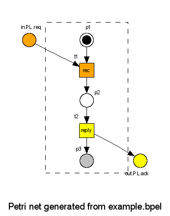
This command creates a file example.dot, containing a Graphviz dot representation of the Petri net, and—if the dot tool was found in the search path—a PNG (Portable Network Graphics) an image file example.png. The latter looks like this:
The graphic depicts the generated open workflow net. The inner of the net, that is, all nodes except the interface places, are depicted inside the dashed box, whereas the interface is depicted outside the frame. Input places and all connected transitions are colored orange. Similarly, output places and connected transitions are colored yellow. Gray places belong to the final marking, that is, the marking [p3] is the final marking of the oWFN.
To reach this final marking, the environment has to send a message in.PL.req, followed by receiving a message out.PL.ack. The name of the communication places is composed by the communication direction (“in” or “out”), the partner link's name (PL) and the operations name (req or ack).
For this very small process, it is easy to validate the generated Petri net model, that is, to compare the intended semantics by the actually modeled semantics. Especially the correlation between the nodes of the Petri net and the activities of the input BPEL process is not obvious for larger processes. To this end,
bpel2owfn -i example.bpel -m petrinet -p small -f info |
displays an information file, consisting of all the Petri net nodes' roles.
PLACES:
ID TYPE ROLES
p1 internal 1.internal.initial
7.initial
7.internal.initial
8.initial
8.internal.initial
p2 internal 8.final
8.internal.final
9.initial
9.internal.initial
p3 internal 1.internal.final
7.final
7.internal.final
9.final
9.internal.final
in.PL.req input in.PL.req
out.PL.ack output out.PL.ack
TRANSITIONS:
ID ROLES
t1 8.internal.receive
t2 9.internal.reply
This file has to be read as follows: the place p1 has the type internal (i.e., is not
connected with an interface place) and has the roles 1.internal.initial, 7.initial,
7.internal.initial, 8.initial, and 8.internal.initial. While the prefix of
each role is the identifier of an activity (1 for the <process>, 7 for the
<sequence>, and 8 for the <receive>), the suffix specifies the role inside the
respective pattern. Without going too much into details, 1.internal.initial is the role of
the initial place of the pattern for the <process>, whereas, for example
7.internal.final is the final place of the <sequence>'s pattern. Similarly, roles of
transitions are specified. Multiple roles of a single place arise due to the merging of distinct
places during the composition of the several patterns.
Now that we have convinced ourselves that the generated net reflects the intended behavior of the BPEL process, we can export the Petri net model to an output file to process it by analysis tools. In this case, we want to create a Fiona open workflow net executing
bpel2owfn -i example.bpel -m petrinet -p small -f owfn -o |
which creates a file example.owfn:
{
generated by: BPEL2oWFN 2.0.1
input file: `example.bpel' (process `exampleprocess')
invocation: `bpel2owfn -i example.bpel -m petrinet -p small -f owfn'
net size: |P|=5, |P_in|= 1, |P_out|= 1, |T|=2, |F|=6
}
PLACE
INTERNAL
p1, p2, p3;
INPUT
in.PL.req {$ MAX_OCCURRENCES = 1 $};
OUTPUT
out.PL.ack {$ MAX_OCCURRENCES = 1 $};
INITIALMARKING
p1: 1 {initial place};
FINALMARKING
p3 {final place};
TRANSITION t1 { input }
CONSUME in.PL.req, p1;
PRODUCE p2;
TRANSITION t2 { output }
CONSUME p2;
PRODUCE out.PL.ack, p3;
{ END OF FILE `example.owfn' }
This is finally the oWFN model of the BPEL process that can be analyzed by Fiona1.
������������������������������������������������������������GNU-Free-Documentation-License.html�����������������������������������������������������������������0000644�0000765�0000765�00000060344�10634503370�017733� 0����������������������������������������������������������������������������������������������������ustar �niels���������������������������niels���������������������������0000000�0000000������������������������������������������������������������������������������������������������������������������������������������������������������������������������ Copyright © 2000,2001,2002 Free Software Foundation, Inc.
51 Franklin St, Fifth Floor, Boston, MA 02110-1301, USA
Everyone is permitted to copy and distribute verbatim copies
of this license document, but changing it is not allowed.
The purpose of this License is to make a manual, textbook, or other functional and useful document free in the sense of freedom: to assure everyone the effective freedom to copy and redistribute it, with or without modifying it, either commercially or noncommercially. Secondarily, this License preserves for the author and publisher a way to get credit for their work, while not being considered responsible for modifications made by others.
This License is a kind of “copyleft”, which means that derivative works of the document must themselves be free in the same sense. It complements the GNU General Public License, which is a copyleft license designed for free software.
We have designed this License in order to use it for manuals for free software, because free software needs free documentation: a free program should come with manuals providing the same freedoms that the software does. But this License is not limited to software manuals; it can be used for any textual work, regardless of subject matter or whether it is published as a printed book. We recommend this License principally for works whose purpose is instruction or reference.
This License applies to any manual or other work, in any medium, that contains a notice placed by the copyright holder saying it can be distributed under the terms of this License. Such a notice grants a world-wide, royalty-free license, unlimited in duration, to use that work under the conditions stated herein. The “Document”, below, refers to any such manual or work. Any member of the public is a licensee, and is addressed as “you”. You accept the license if you copy, modify or distribute the work in a way requiring permission under copyright law.
A “Modified Version” of the Document means any work containing the Document or a portion of it, either copied verbatim, or with modifications and/or translated into another language.
A “Secondary Section” is a named appendix or a front-matter section of the Document that deals exclusively with the relationship of the publishers or authors of the Document to the Document's overall subject (or to related matters) and contains nothing that could fall directly within that overall subject. (Thus, if the Document is in part a textbook of mathematics, a Secondary Section may not explain any mathematics.) The relationship could be a matter of historical connection with the subject or with related matters, or of legal, commercial, philosophical, ethical or political position regarding them.
The “Invariant Sections” are certain Secondary Sections whose titles are designated, as being those of Invariant Sections, in the notice that says that the Document is released under this License. If a section does not fit the above definition of Secondary then it is not allowed to be designated as Invariant. The Document may contain zero Invariant Sections. If the Document does not identify any Invariant Sections then there are none.
The “Cover Texts” are certain short passages of text that are listed, as Front-Cover Texts or Back-Cover Texts, in the notice that says that the Document is released under this License. A Front-Cover Text may be at most 5 words, and a Back-Cover Text may be at most 25 words.
A “Transparent” copy of the Document means a machine-readable copy, represented in a format whose specification is available to the general public, that is suitable for revising the document straightforwardly with generic text editors or (for images composed of pixels) generic paint programs or (for drawings) some widely available drawing editor, and that is suitable for input to text formatters or for automatic translation to a variety of formats suitable for input to text formatters. A copy made in an otherwise Transparent file format whose markup, or absence of markup, has been arranged to thwart or discourage subsequent modification by readers is not Transparent. An image format is not Transparent if used for any substantial amount of text. A copy that is not “Transparent” is called “Opaque”.
Examples of suitable formats for Transparent copies include plain ascii without markup, Texinfo input format, LaTeX input format, SGML or XML using a publicly available DTD, and standard-conforming simple HTML, PostScript or PDF designed for human modification. Examples of transparent image formats include PNG, XCF and JPG. Opaque formats include proprietary formats that can be read and edited only by proprietary word processors, SGML or XML for which the DTD and/or processing tools are not generally available, and the machine-generated HTML, PostScript or PDF produced by some word processors for output purposes only.
The “Title Page” means, for a printed book, the title page itself, plus such following pages as are needed to hold, legibly, the material this License requires to appear in the title page. For works in formats which do not have any title page as such, “Title Page” means the text near the most prominent appearance of the work's title, preceding the beginning of the body of the text.
A section “Entitled XYZ” means a named subunit of the Document whose title either is precisely XYZ or contains XYZ in parentheses following text that translates XYZ in another language. (Here XYZ stands for a specific section name mentioned below, such as “Acknowledgements”, “Dedications”, “Endorsements”, or “History”.) To “Preserve the Title” of such a section when you modify the Document means that it remains a section “Entitled XYZ” according to this definition.
The Document may include Warranty Disclaimers next to the notice which states that this License applies to the Document. These Warranty Disclaimers are considered to be included by reference in this License, but only as regards disclaiming warranties: any other implication that these Warranty Disclaimers may have is void and has no effect on the meaning of this License.
You may copy and distribute the Document in any medium, either commercially or noncommercially, provided that this License, the copyright notices, and the license notice saying this License applies to the Document are reproduced in all copies, and that you add no other conditions whatsoever to those of this License. You may not use technical measures to obstruct or control the reading or further copying of the copies you make or distribute. However, you may accept compensation in exchange for copies. If you distribute a large enough number of copies you must also follow the conditions in section 3.
You may also lend copies, under the same conditions stated above, and you may publicly display copies.
If you publish printed copies (or copies in media that commonly have printed covers) of the Document, numbering more than 100, and the Document's license notice requires Cover Texts, you must enclose the copies in covers that carry, clearly and legibly, all these Cover Texts: Front-Cover Texts on the front cover, and Back-Cover Texts on the back cover. Both covers must also clearly and legibly identify you as the publisher of these copies. The front cover must present the full title with all words of the title equally prominent and visible. You may add other material on the covers in addition. Copying with changes limited to the covers, as long as they preserve the title of the Document and satisfy these conditions, can be treated as verbatim copying in other respects.
If the required texts for either cover are too voluminous to fit legibly, you should put the first ones listed (as many as fit reasonably) on the actual cover, and continue the rest onto adjacent pages.
If you publish or distribute Opaque copies of the Document numbering more than 100, you must either include a machine-readable Transparent copy along with each Opaque copy, or state in or with each Opaque copy a computer-network location from which the general network-using public has access to download using public-standard network protocols a complete Transparent copy of the Document, free of added material. If you use the latter option, you must take reasonably prudent steps, when you begin distribution of Opaque copies in quantity, to ensure that this Transparent copy will remain thus accessible at the stated location until at least one year after the last time you distribute an Opaque copy (directly or through your agents or retailers) of that edition to the public.
It is requested, but not required, that you contact the authors of the Document well before redistributing any large number of copies, to give them a chance to provide you with an updated version of the Document.
You may copy and distribute a Modified Version of the Document under the conditions of sections 2 and 3 above, provided that you release the Modified Version under precisely this License, with the Modified Version filling the role of the Document, thus licensing distribution and modification of the Modified Version to whoever possesses a copy of it. In addition, you must do these things in the Modified Version:
If the Modified Version includes new front-matter sections or appendices that qualify as Secondary Sections and contain no material copied from the Document, you may at your option designate some or all of these sections as invariant. To do this, add their titles to the list of Invariant Sections in the Modified Version's license notice. These titles must be distinct from any other section titles.
You may add a section Entitled “Endorsements”, provided it contains nothing but endorsements of your Modified Version by various parties—for example, statements of peer review or that the text has been approved by an organization as the authoritative definition of a standard.
You may add a passage of up to five words as a Front-Cover Text, and a passage of up to 25 words as a Back-Cover Text, to the end of the list of Cover Texts in the Modified Version. Only one passage of Front-Cover Text and one of Back-Cover Text may be added by (or through arrangements made by) any one entity. If the Document already includes a cover text for the same cover, previously added by you or by arrangement made by the same entity you are acting on behalf of, you may not add another; but you may replace the old one, on explicit permission from the previous publisher that added the old one.
The author(s) and publisher(s) of the Document do not by this License give permission to use their names for publicity for or to assert or imply endorsement of any Modified Version.
You may combine the Document with other documents released under this License, under the terms defined in section 4 above for modified versions, provided that you include in the combination all of the Invariant Sections of all of the original documents, unmodified, and list them all as Invariant Sections of your combined work in its license notice, and that you preserve all their Warranty Disclaimers.
The combined work need only contain one copy of this License, and multiple identical Invariant Sections may be replaced with a single copy. If there are multiple Invariant Sections with the same name but different contents, make the title of each such section unique by adding at the end of it, in parentheses, the name of the original author or publisher of that section if known, or else a unique number. Make the same adjustment to the section titles in the list of Invariant Sections in the license notice of the combined work.
In the combination, you must combine any sections Entitled “History” in the various original documents, forming one section Entitled “History”; likewise combine any sections Entitled “Acknowledgements”, and any sections Entitled “Dedications”. You must delete all sections Entitled “Endorsements.”
You may make a collection consisting of the Document and other documents released under this License, and replace the individual copies of this License in the various documents with a single copy that is included in the collection, provided that you follow the rules of this License for verbatim copying of each of the documents in all other respects.
You may extract a single document from such a collection, and distribute it individually under this License, provided you insert a copy of this License into the extracted document, and follow this License in all other respects regarding verbatim copying of that document.
A compilation of the Document or its derivatives with other separate and independent documents or works, in or on a volume of a storage or distribution medium, is called an “aggregate” if the copyright resulting from the compilation is not used to limit the legal rights of the compilation's users beyond what the individual works permit. When the Document is included in an aggregate, this License does not apply to the other works in the aggregate which are not themselves derivative works of the Document.
If the Cover Text requirement of section 3 is applicable to these copies of the Document, then if the Document is less than one half of the entire aggregate, the Document's Cover Texts may be placed on covers that bracket the Document within the aggregate, or the electronic equivalent of covers if the Document is in electronic form. Otherwise they must appear on printed covers that bracket the whole aggregate.
Translation is considered a kind of modification, so you may distribute translations of the Document under the terms of section 4. Replacing Invariant Sections with translations requires special permission from their copyright holders, but you may include translations of some or all Invariant Sections in addition to the original versions of these Invariant Sections. You may include a translation of this License, and all the license notices in the Document, and any Warranty Disclaimers, provided that you also include the original English version of this License and the original versions of those notices and disclaimers. In case of a disagreement between the translation and the original version of this License or a notice or disclaimer, the original version will prevail.
If a section in the Document is Entitled “Acknowledgements”, “Dedications”, or “History”, the requirement (section 4) to Preserve its Title (section 1) will typically require changing the actual title.
You may not copy, modify, sublicense, or distribute the Document except as expressly provided for under this License. Any other attempt to copy, modify, sublicense or distribute the Document is void, and will automatically terminate your rights under this License. However, parties who have received copies, or rights, from you under this License will not have their licenses terminated so long as such parties remain in full compliance.
The Free Software Foundation may publish new, revised versions of the GNU Free Documentation License from time to time. Such new versions will be similar in spirit to the present version, but may differ in detail to address new problems or concerns. See http://www.gnu.org/copyleft/.
Each version of the License is given a distinguishing version number. If the Document specifies that a particular numbered version of this License “or any later version” applies to it, you have the option of following the terms and conditions either of that specified version or of any later version that has been published (not as a draft) by the Free Software Foundation. If the Document does not specify a version number of this License, you may choose any version ever published (not as a draft) by the Free Software Foundation.
To use this License in a document you have written, include a copy of the License in the document and put the following copyright and license notices just after the title page:
Copyright (C) year your name.
Permission is granted to copy, distribute and/or modify this document
under the terms of the GNU Free Documentation License, Version 1.2
or any later version published by the Free Software Foundation;
with no Invariant Sections, no Front-Cover Texts, and no Back-Cover
Texts. A copy of the license is included in the section entitled ``GNU
Free Documentation License''.
If you have Invariant Sections, Front-Cover Texts and Back-Cover Texts, replace the “with...Texts.” line with this:
with the Invariant Sections being list their titles, with
the Front-Cover Texts being list, and with the Back-Cover Texts
being list.
If you have Invariant Sections without Cover Texts, or some other combination of the three, merge those two alternatives to suit the situation.
If your document contains nontrivial examples of program code, we recommend releasing these examples in parallel under your choice of free software license, such as the GNU General Public License, to permit their use in free software. ��������������������������������������������������������������������������������������������������������������������������������������������������������������������������������������������������������������������������������������������������������������������������������������������Introducing-BPEL2oWFN.html��������������������������������������������������������������������������0000644�0000765�0000765�00000014677�10634503370�016065� 0����������������������������������������������������������������������������������������������������ustar �niels���������������������������niels���������������������������0000000�0000000������������������������������������������������������������������������������������������������������������������������������������������������������������������������
BPEL2oWFN translates a web service expressed in WS-BPEL (Web Service Business Process Execution Language) into an oWFN (open Workflow Net). This oWFN can be used to:
Furthermore, BPEL2oWFN can translate a BPEL4Chor choreography to a Petri net model. This model can be used to analyze properties of a complete choreography or to synthesize a fitting service for an incomplete choreography.
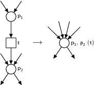
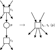
BPEL2oWFN uses static analysis to make the generated Petri net model as compact as possible to analyze a chosen property. This is called flexible model generation. Furthermore, several design flaws can be detected using control and data flow analysis.
BPEL2oWFN was written by Niels Lohmann, Christian Gierds and Martin Znamirowski. It is part of the Tools4BPEL project funded by the Bundesministerium f�r Bildung und Forschung. See http://www.informatik.hu-berlin.de/top/tools4bpel for details.
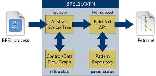
| Input BPEL Process |
BPEL2oWFN can read BPEL processes compliant to the WS-BPEL 2.0
or the BPEL4WS 1.1 specification.
|
| Abstract Syntax Tree |
The AST (abstract syntax tree) is the main data structure of BPEL2oWFN.
The AST is annotated with information gained by static analysis.
|
| Control/Data Flow Graph |
From the abstract syntax tree, a control/data flow graph is built. This graph
is used to apply static analysis algorithms to gain information
(e.g., dead code) about the process. These algorithms Furthermore, design
flaws such as cyclic control links or conflicting receiving activities are
detected.
|
| Petri Net API |
The annotated abstract syntax tree is used to generate a Petri net model of the
BPEL process. All Petri net-related functions (adding, removing and
merging of nodes; structural reduction) are provided by the Petri net
API (application programming interface).
|
| Pattern Repository |
For each BPEL construct, several patterns with different degrees of
abstraction are stored in the pattern repository. Using the information gained
by static analysis, the most abstract pattern applicable is used.
|
| Output Petri Net |
The generated Petri net model can be exported to many file formats, such as
PNML, LoLA, Fiona oWFN, INA, APNN, or PEP.
|
The standard invocation of BPEL2oWFN is:
bpel2owfn -i service.bpel -m petrinet -f owfn -o
where service.bpel is a BPEL process. The option -f owfn causes BPEL2oWFN to generate an open workflow net (option -m petrinet). This net is written to a file named service.owfn, because of the option -o.
BPEL2oWFN can be called without any parameter. In this case, it acts
as a simple parser for BPEL processes that reads its input from the
standard input (stdin).
BPEL2oWFN supports the following command-line options:
stdin). Wildcards such as process*.bpel are also allowed.
stdout).
stderr).
Debug level:
When invoking BPEL2oWFN several modes are possible.
For examples, check test/bpel4chor directory. When combined with LoLA file output, an additional .task file is generated. With the help of this file LoLA can check for weak termination of the composition.
Note that the choreography mode is only tested with the small mode.
To support the translation of a BPEL4Chor choreography, a participant topology
can be additionally parsed using the topology parameter.
At most one mode can be selected. If no mode is given, BPEL2oWFN acts like a plain BPEL parser; that is, the input file is read, but no output is generated.
These options control some Petri net-related options.
<exit>, <throw>, <compensate>, <compensateScope> activities) is not translated to
the Petri net model. When combined with reduce, this parameter yields
the most compact Petri net model.
<throw> activities, and
join failures can occur. With the standardfaults parameter, also the
occurrence of other BPEL standard faults is modeled. This parameter
yields the most-detailled, and thus biggest Petri net model.
If you want to enable more than one parameter you have to add -p/ --parameter to each parameter.
Especially for the Petri net mode, a variaty of output formats are supported. There are invoked by the following option:
<type> tag
which is only supported by Yasper3. When the parameter -o is used, a
file with the suffix .pnml is created.
In any case, when the tool dot is found in the search path during
configuration of BPEL2oWFN and the parameter -o is used,
dot is used to generate a PNG (Portable Network Image) file.
In this case, two files with the suffixes .dot and .png are
created. Note that when the ast mode is used with the dot file
format, the -o parameter has to be used.
In this section we show some examples how BPEL2oWFN can be invoked. See File Formats for more examples.
dot which layouts the Petri net and creates an output
PostScript file sample.ps.
Further examples for invocations of BPEL2oWFN can be found in the tests directory of the source distribution.
[1] This mode was formally called consinstency.
[2] This mode was formally called communicationonly.
[3] Yasper is available at http://www.yasper.org.
BPEL2oWFN performs several analysis steps on the input BPEL process. These messages are displayed during parsing and postprocessing of the process, and can be classified as follows:
An example for a message is this:
CubeManagement.bpel:566 - [W00114]
variable `waitResponse' used as `variable' in <from> might be uninitialized
The first line contains the filename of the input process CubeManagement.bpel and the line number 566 of the displayed issue. The line number might be imprecise; that is, it might deviate up or down a few lines. After the line number, the error code is displayed. W00114 stands for a warning with code 114. The detailed description of the messages can be suppressed with option -d0.
Further details can be taken from the table below.
| Code | Type | Description
|
|---|---|---|
| 2 | static analysis |
A WS-BPEL processor MUST reject any WSDL portType definition that includes
overloaded operation names.1
|
| 3 | static analysis |
If the value of exitOnStandardFault of a <scope> or <process>
is set to "yes", then a fault handler that explicitly targets the WS-BPEL
standard faults MUST NOT be used in that scope.
|
| 6 | static analysis |
The <rethrow> activity MUST only be used within a faultHandler (i.e.
<catch> and <catchAll> elements).
|
| 5 | static analysis |
If the portType attribute is included for readability, in a <receive>,
<reply>, <invoke>, <onEvent> or <onMessage>
element, the value of the portType attribute MUST match the portType
value implied by the combination of the specified partnerLink and the role
implicitly specified by the activity.
|
| 7 | static analysis |
The <compensateScope> activity MUST only be used from within a
faultHandler, another compensationHandler, or a
terminationHandler.
|
| 8 | static analysis |
The <compensate> activity MUST only be used from within a
faultHandler, another compensationHandler, or a
terminationHandler.
|
| 15 | static analysis |
To be instantiated, an executable business process MUST contain at least one
<receive> or <pick> activity annotated with a
createInstance="yes" attribute.
|
| 16 | static analysis |
A partnerLink MUST specify the myRole or the partnerRole,
or both.
|
| 17 | static analysis |
The initializePartnerRole attribute MUST NOT be used on a partnerLink
that does not have a partner role.
|
| 18 | static analysis |
The name of a partnerLink MUST be unique among the names of all
partnerLinks defined within the same immediately enclosing scope.
|
| 23 | static analysis |
The name of a variable MUST be unique among the names of all variables defined
within the same immediately enclosing scope.
|
| 24 | static analysis |
Variable names are BPELVariableNames, that is, NCNames (as defined in
XML Schema specification) but in addition they MUST NOT contain the
. character.
|
| 25 | static analysis |
The messageType, type or element attributes are used to specify
the type of a variable. Exactly one of these attributes MUST be used.
|
| 32 | static analysis |
For <assign>, the <from> and <to> element MUST be one
of the specified variants.2
|
| 35 | static analysis |
In the from-spec of the partnerLink variant of <assign> the value
"myRole" for attribute endpointReference is only permitted when the
partnerLink specifies the attribute myRole.
|
| 36 | static analysis |
In the from-spec of the partnerLink variant of <assign> the value
"partnerRole" for attribute endpointReference is only permitted
when the partnerLink specifies the attribute partnerRole.
|
| 37 | static analysis |
In the to-spec of the partnerLink variant of <assign> only partnerLinks
are permitted which specify the attribute partnerRole.
|
| 44 | static analysis |
The name of a <correlationSet> MUST be unique among the names of all
<correlationSet> defined within the same immediately enclosing scope.
|
| 51 | static analysis |
The inputVariable attribute MUST NOT be used on an Invoke
activity that contains <toPart> elements.
|
| 52 | static analysis |
The outputVariable attribute MUST NOT be used on an Invoke
activity that contains <toPart> elements.
|
| 55 | static analysis |
For <receive>, if <fromPart> elements are used on a
<receive> activity then the variable attribute MUST NOT be used on the
same activity.
|
| 56 | static analysis |
A “start activity” is a <receive> or <pick> activity that is
annotated with a createInstance="yes" attribute. Activities other than
the following: start activities, <scope>, <flow> and
<sequence> MUST NOT be performed prior to or simultaneously with start
activities.
|
| 57 | static analysis |
If a process has multiple start activities with correlation sets then all such
activities MUST share at least one common correlationSet and all common
correlationSets defined on all the activities MUST have the value of the
initiate attribute be set to "join".
|
| 59 | static analysis |
For <reply>, if <toPart> elements are used on a <reply>
activity then the variable attribute MUST NOT be used on the same
activity.
|
| 62 | static analysis |
If <pick> has a createInstance attribute with a value of
yes, the events in the <pick> MUST all be <onMessage>
events.
|
| 63 | static analysis |
The semantics of the <onMessage> event are identical to a
<receive> activity regarding the optional nature of the variable
attribute or <fromPart> elements, if <fromPart> elements on an
activity then the variable attribute MUST NOT be used on the same activity
(see SA00055).
|
| 64 | static analysis |
For <flow>, a declared link's name MUST be unique among all
<link> names defined within the same immediately enclosing
<flow>.
|
| 65 | static analysis |
The value of the linkName attribute of <source> or
<target> MUST be the name of a <link> declared in an enclosing
<flow> activity.
|
| 66 | static analysis |
Every link declared within a <flow> activity MUST have exactly one
activity within the <flow> as its source and exactly one activity within
the <flow> as its target.
|
| 67 | static analysis |
Two different links MUST NOT share the same source and target activities; that
is, at most one link may be used to connect two activities.
|
| 68 | static analysis |
An activity MAY declare itself to be the source of one or more links by
including one or more <source> elements. Each <source>
element MUST use a distinct link name.
|
| 69 | static analysis |
An activity MAY declare itself to be the target of one or more links by
including one or more <target> elements. Each <target> element
associated with a given activity MUST use a link name distinct from all other
<target> elements at that activity.
|
| 70 | static analysis |
A link MUST NOT cross the boundary of a repeatable construct or the
<compensationHandler> element. This means, a link used within a
repeatable construct (<while>, <repeatUntil>, <forEach>,
<eventHandlers>) or a <compensationHandler> MUST be declared in
a <flow> that is itself nested inside the repeatable construct or
<compensationHandler>.
|
| 71 | static analysis |
A link that crosses a <catch>, <catchAll> or
<terminationHandler> element boundary MUST be outbound only, that is,
it MUST have its source activity within the <faultHandlers> or
<terminationHandler>, and its target activity outside of the scope
associated with the handler.
|
| 72 | static analysis |
A <link> declared in a <flow> MUST NOT create a control cycle,
that is, the source activity must not have the target activity as a logically
preceding activity.3
|
| 73 | static analysis |
The expression for a join condition MUST be constructed using only Boolean
operators and the activity's incoming links' status values.
|
| 74 | static analysis |
The expressions in <startCounterValue> and <finalCounterValue>
MUST return a TII (meaning they contain at least one character) that can be
validated as a xsd:unsignedInt. Static analysis MAY be used to detect
this erroneous situation at design time when possible (for example, when the
expression is a constant).
|
| 75 | static analysis |
For the <forEach> activity, <branches> is an integer value
expression. Static analysis MAY be used to detect if the integer value is
larger than the number of directly enclosed activities of <forEach> at
design time when possible (for example, when the branches expression is a
constant).
|
| 76 | static analysis |
For <forEach> the enclosed scope MUST NOT declare a variable with the
same name as specified in the counterName attribute of
<forEach>.
|
| 77 | static analysis |
The value of the target attribute on a <compensateScope>
activity MUST refer to the name of an immediately enclosed scope of the
scope containing the FCT-handler with the <compensateScope>
activity. This includes immediately enclosed scopes of an event handler
(<onEvent> or <onAlarm>) associated with the same scope.
|
| 78 | static analysis |
The target attribute of a <compensateScope> activity MUST refer
to a scope or an invoke activity with a fault handler or
compensation handler.
|
| 79 | static analysis |
The root scope inside a FCT-handler MUST not have a compensation
handler.
|
| 80 | static analysis |
There MUST be at least one <catch> or <catchAll> element within
a <faultHandlers> element.
|
| 81 | static analysis |
For the <catch> construct; to have a defined type associated with the
fault variable, the faultVariable attribute MUST only be used if either
the faultMessageType or faultElement attributes, but not both,
accompany it. The faultMessageType and faultElement attributes
MUST NOT be used unless accompanied by faultVariable attribute.
|
| 82 | static analysis |
The peer-scope dependency relation MUST NOT include cycles. In other words,
WS-BPEL forbids a process in which there are peer scopes S1 and S2
such that S1 has a peer-scope dependency on S2 and S2 has a peer-scope
dependency on S1.4
|
| 83 | static analysis |
An event handler MUST contain at least one <onEvent> or
<onAlarm> element.
|
| 84 | static analysis |
The partnerLink reference of <onEvent> MUST resolve to a partner
link declared in the process in the following order: the associated scope
first and then the ancestor scopes.
|
| 88 | static analysis |
For <onEvent>, the resolution order of the correlation set(s)
referenced by <correlation> MUST be first the associated scope and then
the ancestor scopes.
|
| 91 | static analysis |
A scope with the isolated attribute set to "yes" is called an
isolated scope. Isolated scopes MUST NOT contain other isolated scopes.
|
| 92 | static analysis |
Within a scope, the name of all named immediately enclosed scopes MUST be
unique.
|
| 93 | static analysis |
Identical <catch> constructs MUST NOT exist within a
<faultHandlers> element.
|
| 100 | notice |
Either a non-standard element5 was parsed
or a BPEL activity was considered as
misplaced. In the first case, a non-standard element was parsed when the
parser expected a BPEL standard activity. Then, a syntax error is
printed and the whole element is ignored. The parse error and this message
can usually be ignored, as non-standard elements would neither we translated
to a Petri net model nor are constrained by the WS-BPEL
specification.
In the second case, a syntactically correct BPEL
was skipped, because it was misplaced. As an example, consider two activities
embedded in a |
| 101 | notice |
The <partners> construct (only supported by BPEL4WS 1.1) is skipped due
to a syntax error.
|
| 102 | notice |
The <to> or <from> construct is skipped due to a syntax error.
|
| 103 | notice |
The <condition> construct is skipped due to a syntax error.
|
| 104 | critical |
When a syntax error occurs, BPEL2oWFN tries to recover and continues parsing the
input file after skipping the faulty or unknown element. Sometimes, however,
the skipping of activities yields to situations where a further analysis of the
BPEL process is impossible. In this case, the syntax of the process
has to be fixed or non-standard elements have to be removed or out-commented.
|
| 105 | notice |
When a syntax error occurs, BPEL2oWFN tries to recover and continues parsing the
input file after skipping the faulty or unknown element. If it is possible to
continue, the analysis results might be faulty. In this case, the syntax of the
process has to be fixed or non-standard elements have to be removed or
out-commented.
|
| 106 | warning |
CFG analysis detected two receiving activities (i.e., <receive>,
<onEvent>, <onMessage>, synchronous <invoke>) that might
be activated concurrently and share the same partner link, port type, operation,
and correlation set. When a message is sent to the process, these activities
are in conflict; that is, it is not defined which activity will receive an
inbound message. At runtime, the standard fault bpel:conflictingReceive
would be thrown.6
|
| 107 | warning |
A mandatory attribute of an activity was not defined. Especially for
communicating activities, the absence of partnerLink and
operation might hamper the subsequent analysis and Petri net generation.
|
| 108 | syntax |
An attribute was set to a value that violates the attribute's given type. Only
the types tBoolean, tInitiate, tRoles, and
tPattern are checked.
|
| 109 | warning |
A variable referenced in an activity was not defined before; that is, no
matching <variable> definition was found in a parent scope.
|
| 110 | warning |
A partner link referenced in an activity was not defined before; that is, no
matching <partnerLink> definition was found in the process.
|
| 111 | warning |
A correlation set referenced in an activity was not defined before; that is, no
matching <correlationSet> definition was found in a parent scope.
|
| 112 | notice |
The <literal> construct is skipped due to a syntax error.
|
| 113 | syntax |
A UTF-8 character was read in the input file. As BPEL2oWFN's scanner does not
support Unicode, all UTF-8 characters are ignored. This message is only
displayed when the first UTF-8 character is read.
|
| 114 | warning |
CFG analysis detected a read access to a variable that was not
initialized before. At runtime, the standard fault
bpel:uninitializedVariable would be thrown.7
|
| 115 | notice |
The process definition defines an abstract process profile, and thus allows
several “opaque” constructs. When processing and analyzing an abstract
process, BPEL2oWFN might report error messages that where designed for
executable processes, for example missing attributes. Static analysis errors
detected in an abstract process are reported as warnings.
|
| 116 | notice |
An <opaqueActivity> of an abstract process is modeled by an <empty> activity.
|
| 117 | notice |
When using the parameter small, the occurrence of join
failures is not modeled. Thus, any activity is treated as if the
attribute suppressJoinFailure is set to yes.8
|
| 118 | notice |
A user-defined transition condition is ignored and modeled as “n-out-of-n”
(true) instead.
|
| 119 | notice |
A user-defined transition condition is ignored and modeled as “1-out-of-n”
(XOR) instead.
|
| 120 | notice |
When using the parameter small, the FTC (fault, termination,
and compensation) handlers are not modeled.
|
| 121 | notice |
When using the parameter small, activities of the negative
control flow (<exit>, <throw>, <compensate>, and
<compensateScope>) are replaced by an <empty> activity.
|
| 122 | notice |
A syntax error in the BPEL4Chor chorography file occurred.
|
| 123 | notice |
A syntax error in the WSDL input file occurred.
|
| 124 | notice |
An XML Schema element nested in a WSDL <types> element was ignored. This is
usually no problem, as WSDL <types> are not evaluated in subsequent analysis
or translation.
|
| 125 | notice |
A variable property element was ignored while parsing the input WSDL file.
|
| 126 | warning |
A WSDL <message> referenced in a WSDL <operation> was not found.
|
| 127 | warning |
A WSDL <portType> referenced in a WSDL <role> was not found.
|
| 128 | warning |
A WSDL <operation> referenced in a BPEL activity was not specified in the
input WSDL file.
|
| 129 | warning |
A WSDL <role> of a partnerLinkType referenced by a <partnerLink> was not
defined in the specified <partnerLinkType> in the input WSDL file.
|
| 130 | warning |
A WSDL <partnerLinkType> referenced by a <partnerLink> was not specified in
the input WSDL file.
|
| 131 | error |
An activity has neither a name or id attribute and thus can not be linked with a BPEL4Chor <messageLink>.
|
| 132 | error |
An activity has neither could not be linked with a BPEL4Chor <messageLink> using the activity's name or id attribute.
|
| 133 | notice |
An <extensionActivity> is replaced by an <opaqueActivity> (cf. notice 116).
|
| 134 | warning |
A BPEL4Chor <participantType> was defined twice.
|
| 135 | warning |
The <participantType> referenced by a BPEL4Chor <participant> was not found.
|
| 136 | error |
The value of a <forEach>'s attribute id or name does not reference a BPEL4Chor
<participant> or <participantSet>. Thus, the <forEach> activity is not grounded to the
BPEL4Chor topology.
|
| 137 | error |
In a BPEL4Chor topology, no XML namespace was defined for a <participant>. In a
WS-BPEL file, the attribute targetNamespace could not to be grounded to a
BPEL4Chor <participant>.
|
| 138 | notice |
In a BPEL4Chor topology, a partner link specified for an activity was not found. Instead,
the name of the specified id is used as a partner link.
|
[1] The descriptions for static analysis messages are taken from Appendix B of the WS-BPEL specification.
[2] The specification describes all allowed combinations of elements and attributes in from- and to-specifications.
[3] This fault can only be detected in mode mode cfg.
[4] This fault can only be detected in mode mode cfg.
[5] All elements that are not explicitly defined in the WS-BPEL specification (e.g., elements from other namespaces) are considered as “non-standard”.
[6] This fault can only be detected in mode mode cfg.
[7] This fault can only be detected in mode mode cfg.
[8] If the attribute suppressJoinFailure is not explicitly defined for an activity, the value is inherited by the parent activity.
About this document:
This manual is for GNU BPEL2oWFN, version 2.0.2, a tool translating a BPEL process into an open workflow net (oWFN), last updated 15 June 2007.
Copyright © 2005, 2006, 2007 Niels Lohmann
Permission is granted to copy, distribute and/or modify this document under the terms of the GNU Free Documentation License, Version 1.2 or any later version published by the Free Software Foundation; with no Invariant Sections, with the Front-Cover Texts being “A GNU Manual,” and with the Back-Cover Texts as in (a) below. A copy of the license is included in the section entitled “GNU Free Documentation License.”(a) The FSF's Back-Cover Text is: “You have freedom to copy and modify this GNU Manual, like GNU software.”
This manual does not explain how to setup or install GNU BPEL2oWFN. For this
information please read the Installation Manual which is part of the
distribution, or can be downloaded from the website of GNU BPEL2oWFN,
http://www.gnu.org/software/bpel2owfn.

GNU BPEL2oWFN was developed during the Tools4BPEL project funded by
the German Federal Ministry for Education and Research (BMBF), see
http://www.informatik.hu-berlin.de/top/tools4bpel for details.