6.3.2.2 Circles and the complex plane 
Before going onto the derivation, it is also useful to review how the complex numbers and their plane relate to the circles we talked about above. The two schematics in the middle and right of Figure 6.1 show how a 1D function of time can be made using the 2D real and imaginary surface. Seeing the animation in Wikipedia will really help in understanding this important concept. At each point in time, we take the vertical coordinate of the point and use it to find the value of the function at that point in time. Figure 6.2 shows this relation with the axes marked.
Leonhard Euler170 (1707 – 1783 A.D.) showed that the complex exponential (\(e^{iv}\) where \(v\) is real) is periodic and can be written as: \(e^{iv}=\cos{v}+isin{v}\). Therefore \(e^{iv+2\pi}=e^{iv}\). Later, Caspar Wessel (mathematician and cartographer 1745 – 1818 A.D.) showed how complex numbers can be displayed as vectors on a plane. Euler’s identity might seem counter intuitive at first, so we will try to explain it geometrically (for deeper physical insight). On the real-imaginary 2D plane (like the left hand plot in each box of Figure 6.2), multiplying a number by \(i\) can be interpreted as rotating the point by \(90\) degrees (for example, the value \(3\) on the real axis becomes \(3i\) on the imaginary axis). On the other hand, \(e\equiv\lim_{n\rightarrow\infty}(1+{1\over n})^n\), therefore, defining \(m\equiv nu\), we get:
$$e^{u}=\lim_{n\rightarrow\infty}\left(1+{1\over n}\right)^{nu} =\lim_{n\rightarrow\infty}\left(1+{u\over nu}\right)^{nu} =\lim_{m\rightarrow\infty}\left(1+{u\over m}\right)^{m}$$
Taking \(u\equiv iv\) the result can be written as a generic complex number (a function of \(v\)):
$$e^{iv}=\lim_{m\rightarrow\infty}\left(1+i{v\over m}\right)^{m}=a(v)+ib(v)$$
For \(v=\pi\), a nice geometric animation of going to the limit can be seen on Wikipedia. We see that \(\lim_{m\rightarrow\infty}a(\pi)=-1\), while \(\lim_{m\rightarrow\infty}b(\pi)=0\), which gives the famous \(e^{i\pi}=-1\) equation. The final value is the real number \(-1\), however the distance of the polygon points traversed as \(m\rightarrow\infty\) is half the circumference of a circle or \(\pi\), showing how \(v\) in the equation above can be interpreted as an angle in units of radians and therefore how \(a(v)=cos(v)\) and \(b(v)=sin(v)\).
Since \(e^{iv}\) is periodic (let’s assume with a period of \(T\)), it is more clear to write it as \(v\equiv{2{\pi}n\over T}t\) (where \(n\) is an integer), so \(e^{iv}=e^{i{2{\pi}n\over T}t}\). The advantage of this notation is that the period (\(T\)) is clearly visible and the frequency (\(2{\pi}n \over T\), in units of 1/cycle) is defined through the integer \(n\). In this notation, \(t\) is in units of “cycle”s.
As we see from the examples in Figure 6.1 and Figure 6.2, for each constituting frequency, we need a respective ‘magnitude’ or the radius of the circle in order to accurately approximate the desired 1D function. The concepts of “period” and “frequency” are relatively easy to grasp when using temporal units like time because this is how we define them in every-day life. However, in an image (astronomical data), we are dealing with spatial units like distance. Therefore, by one “period” we mean the distance at which the signal is identical and frequency is defined as the inverse of that spatial “period”. The complex circle of Figure 6.2 can be thought of the Moon rotating about Earth which is rotating around the Sun; so the “Real (signal)” axis shows the Moon’s position as seen by a distant observer on the Sun as time goes by. Because of the scalar (not having any direction or vector) nature of time, Figure 6.2 is easier to understand in units of time. When thinking about spatial units, mentally replace the “Time (sec)” axis with “Distance (meters)”. Because length has direction and is a vector, visualizing the rotation of the imaginary circle and the advance along the “Distance (meters)” axis is not as simple as temporal units like time.
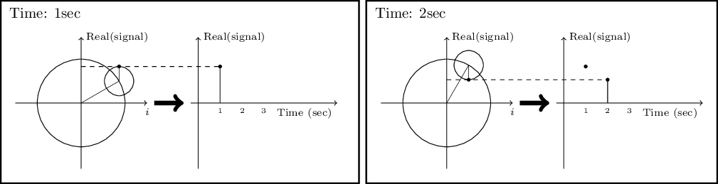
Figure 6.2: Relation between the real (signal), imaginary (\(i\equiv\sqrt{-1}\)) and time axes at two snapshots of time.