3.1 A simple refractor design

3.1.1 Building the optical system
Unlike much optical design software which relies on a list of surfaces to sequentially propagate light through the system, Goptical uses an object representation of the optical system in 3d space.
To model an optical system with Goptical, we just have to instantiate components and add them to the system.
For this refractor example we first need to deal with glass materials used in the design. Our achromatic refractor design needs two lenses of different glass materials. In this example we choose to model Bk7 and F3 glasses with the Sellmeier model:
// code from examples/simple_refractor/refractor.cc:64

  Material::Sellmeier bk7(1.03961212, 6.00069867e-3, 0.231792344,
                          2.00179144e-2, 1.01046945, 1.03560653e2);

  Material::Sellmeier f3(8.23583145e-1, 6.41147253e-12, 7.11376975e-1,
                         3.07327658e-2, 3.12425113e-2, 4.02094988);
The Sys::OpticalSurface class is used to model a single optical surface.
The two lenses have the same disk outline shape, so we declare the shape model once:
  Shape::Disk   lens_shape(100); // lens diameter is 100mm

  // 1st lens, left surface
  Curve::Sphere curve1(2009.753); // spherical curve with given radius of curvature
  Curve::Sphere curve2(-976.245);
Surface curves rely on dedicated models which are not dependent on optical component being used. Here we need two simple spherical curves for the first lens.
The first lens component can then be instantiated. We need to specify its 3d position, thickness, shape model, curve models and material models. Material::none will later be replaced by system environment material.
  Sys::OpticalSurface s1(Math::Vector3(0, 0, 0), // position,
                         curve1, lens_shape,     // curve & aperture shape
                         Material::none, bk7);   // materials

  // 1st lens, right surface
  Sys::OpticalSurface s2(Math::Vector3(0, 0, 31.336),
                         curve2, lens_shape,
                         bk7, Material::none);
More convenient optical surface constructors are available for simple cases, with circular aperture and spherical curvature. They are used for the second lens:
  // 2nd lens, left surface
  Sys::OpticalSurface s3(Math::Vector3(0, 0, 37.765), // position,
                         -985.291, 100,        // roc & circular aperture radius,
                         Material::none, f3);  // materials

  // 2nd lens, right surface
  Sys::OpticalSurface s4(Math::Vector3(0, 0, 37.765+25.109),
                         -3636.839, 100,
                         f3, Material::none);
The Sys::Lens class is more convenient to use for most designs as it can handle a list of surfaces. In this example we choose to use the Sys::OpticalSurface class directly to show how things work. The convenient method is used in the next example.
We then create a point light source at infinite distance with a direction vector aimed at entry surface (left of first lens):
  // light source
  Sys::SourcePoint source(Sys::SourceAtInfinity,
                          Math::Vector3(0, 0, 1));
And we finally create an image plane near the expected focal point:
  // image plane
  Sys::Image    image(Math::Vector3(0, 0, 3014.5),  // position
                      60);                           // square size,
All these components need to be added to an optical system:
  Sys::System   sys;

  // add components
  sys.add(source);
  sys.add(s1);
  sys.add(s2);
  sys.add(s3);
  sys.add(s4);
  sys.add(image);
This simple optical design is ready for ray tracing and analysis.
3.1.2 Performing light propagation
Light propagation through the optical system is performed by the Trace::Tracer class. There are several tracer parameters which can be tweaked before starting light propagation. Some default parameters can be set for an optical system instance; they will be used for each new tracer created for the system.
When light is propagated through the system, a tracer may be instructed to keep track of rays hitting or generated by some of the components for further analysis.
Some analysis classes are provided which embed a tracer configured for a particular analysis, but it's still possible to request a light propagation by directly instantiating a tracer object.
There are two major approaches to trace rays through an optical system:
Sequential ray tracing: This requires an ordered list of surfaces to traverse. Rays are generated by the light source and propagated in the specified sequence order. Any light ray which doesn't reach the next surface in order is lost.
Non-sequential ray tracing: Rays are generated by the light source and each ray interacts with the first optical component found on its path. Rays are propagated this way across system components until they reach an image plane or get lost.
The default behavior in Goptical is to perform a non-sequential ray trace when no sequence is provided.
Non-sequential ray trace
A non-sequential ray trace needs the specification of an entrance pupil so that rays from light sources can be targeted at optical system entry.
Performing light propagation only needs instantiation of a Trace::Tracer object and invocation of its Trace::Tracer::trace function. Tracer parameters are inherited from system default tracer parameters:
  sys.set_entrance_pupil(s1);
  Trace::Tracer tracer(sys);
  tracer.trace();
When performing a non-sequential ray trace, only optical components based on Sys::Surface will interact with light.
All enabled light sources which are part of the system are considered.
Sequential ray trace
Switching to a sequential ray trace is easy: The sequence is setup from components found in the system, in order along the Z axis.
  Trace::Sequence seq(sys);

  sys.get_tracer_params().set_sequential_mode(seq);
More complicated sequences must be created empty and described explicitly using the Trace::Sequence::add function.
Optical system and sequence objects can be displayed using stl streams:
  std::cout << "system:" << std::endl << sys;
  std::cout << "sequence:" << std::endl << seq;
Ray tracing is then performed in the same way as for non-sequential ray traces:
  Trace::Tracer tracer(sys);
  tracer.trace();
When performing a sequential ray trace, all optical components can process incoming light rays.
A single light source must be present at the beginning of the sequence.
3.1.3 Rendering optical layout and rays
The result of ray tracing is stored in a Trace::Result object which stores information about generated and intercepted rays and involved components for each ray. Not all rays' interactions are stored by default, and the result object must be first configured to specify which interactions should be stored for further analysis.
Here we want to draw all rays which are traced through the system. We first have to instruct our Trace::Result object to remember which rays were generated by the source component in the system, so that it can used as a starting point for drawing subsequently scattered and reflected rays.
We use an Io::Renderer based object which is able to draw various things. We use it to draw system components as well as to recursively draw all rays generated by light sources.
Here is what we need to do in order:
Instantiate a renderer object able to write graphics in some output format.
Fit renderer viewport to optical system.
Draw system components.
Optionally change the ray distribution on entrance pupil so that only meridional rays are traced.
Instruct the result object to keep track of rays generated by the source component.
Perform the ray tracing.
Draw traced rays.
  Io::RendererSvg renderer("layout.svg", 1024, 100);

  // draw 2d system layout
  sys.draw_2d_fit(renderer);
  sys.draw_2d(renderer);

  Trace::Tracer tracer(sys);

  // trace and draw rays from source
  tracer.get_params().set_default_distribution(
    Trace::Distribution(Trace::MeridionalDist, 5));
  tracer.get_trace_result().set_generated_save_state(source);
  tracer.trace();
  tracer.get_trace_result().draw_2d(renderer);
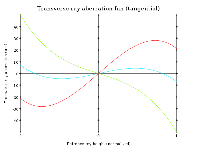
3.1.4 Performing a ray fan analysis
The Analysis namespace contains classes to perform some common analysis on optical systems. Analysis classes may embed a Trace::Tracer object if light propagation is needed to perform analysis.
Ray fan plots can be computed using the Analysis::RayFan class which is able to plot various ray measurements on both 2d plot axes.
The example below shows how to produce a transverse aberration plot by plotting entrance ray height against transverse distance:
  Io::RendererSvg     renderer("fan.svg", 640, 480, Io::rgb_white);

  Analysis::RayFan    fan(sys);

  // select light source wavelens
  source.clear_spectrum();
  source.add_spectral_line(Light::SpectralLine::C);
  source.add_spectral_line(Light::SpectralLine::e);
  source.add_spectral_line(Light::SpectralLine::F);

  // get transverse aberration plot
  ref<Data::Plot> fan_plot = fan.get_plot(Analysis::RayFan::EntranceHeight,
                                          Analysis::RayFan::TransverseDistance);

  fan_plot->draw(renderer);