15.2.2 Three-Dimensional Plots 
The function mesh produces mesh surface plots. For example,
tx = ty = linspace (-8, 8, 41)';
[xx, yy] = meshgrid (tx, ty);
r = sqrt (xx .^ 2 + yy .^ 2) + eps;
tz = sin (r) ./ r;
mesh (tx, ty, tz);
xlabel ("tx");
ylabel ("ty");
zlabel ("tz");
title ("3-D Sombrero plot");
produces the familiar “sombrero” plot shown in Figure 15.5. Note
the use of the function meshgrid to create matrices of X and Y
coordinates to use for plotting the Z data. The ndgrid function
is similar to meshgrid, but works for N-dimensional matrices.
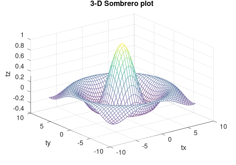
Figure 15.5: Mesh plot.
The meshc function is similar to mesh, but also produces a
plot of contours for the surface.
The plot3 function displays arbitrary three-dimensional data,
without requiring it to form a surface. For example,
t = 0:0.1:10*pi;
r = linspace (0, 1, numel (t));
z = linspace (0, 1, numel (t));
plot3 (r.*sin (t), r.*cos (t), z);
xlabel ("r.*sin (t)");
ylabel ("r.*cos (t)");
zlabel ("z");
title ("plot3 display of 3-D helix");
displays the spiral in three dimensions shown in Figure 15.6.
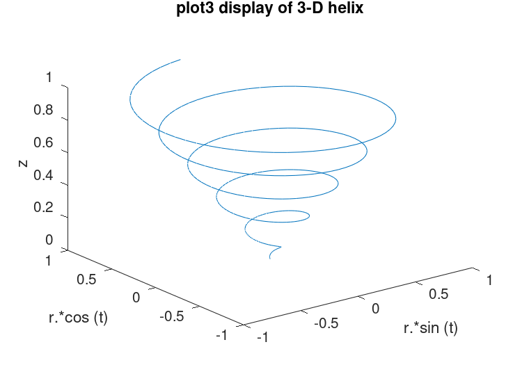
Figure 15.6: Three-dimensional spiral.
Finally, the view function changes the viewpoint for
three-dimensional plots.
- : mesh
(x, y, z)¶ - : mesh
(z)¶ - : mesh
(…, c)¶ - : mesh
(…, prop, val, …)¶ - : mesh
(hax, …)¶ - :
h =mesh(…)¶ Plot a 3-D wireframe mesh.
The wireframe mesh is plotted using rectangles. The vertices of the rectangles [x, y] are typically the output of
meshgrid. over a 2-D rectangular region in the x-y plane. z determines the height above the plane of each vertex. If only a single z matrix is given, then it is plotted over the meshgridx = 1:columns (z), y = 1:rows (z). Thus, columns of z correspond to different x values and rows of z correspond to different y values.The color of the mesh is computed by linearly scaling the z values to fit the range of the current colormap. Use
caxisand/or change the colormap to control the appearance.Optionally, the color of the mesh can be specified independently of z by supplying a color matrix, c.
Any property/value pairs are passed directly to the underlying surface object. The full list of properties is documented at Surface Properties.
If the first argument hax is an axes handle, then plot into this axes, rather than the current axes returned by
gca.The optional return value h is a graphics handle to the created surface object.
See also: ezmesh, meshc, meshz, trimesh, contour, surf, surface, meshgrid, hidden, shading, colormap, caxis.
- : meshc
(x, y, z)¶ - : meshc
(z)¶ - : meshc
(…, c)¶ - : meshc
(…, prop, val, …)¶ - : meshc
(hax, …)¶ - :
h =meshc(…)¶ Plot a 3-D wireframe mesh with underlying contour lines.
The wireframe mesh is plotted using rectangles. The vertices of the rectangles [x, y] are typically the output of
meshgrid. over a 2-D rectangular region in the x-y plane. z determines the height above the plane of each vertex. If only a single z matrix is given, then it is plotted over the meshgridx = 1:columns (z), y = 1:rows (z). Thus, columns of z correspond to different x values and rows of z correspond to different y values.The color of the mesh is computed by linearly scaling the z values to fit the range of the current colormap. Use
caxisand/or change the colormap to control the appearance.Optionally the color of the mesh can be specified independently of z by supplying a color matrix, c.
Any property/value pairs are passed directly to the underlying surface object. The full list of properties is documented at Surface Properties.
If the first argument hax is an axes handle, then plot into this axes, rather than the current axes returned by
gca.The optional return value h is a 2-element vector with a graphics handle to the created surface object and to the created contour plot.
See also: ezmeshc, mesh, meshz, contour, surfc, surface, meshgrid, hidden, shading, colormap, caxis.
- : meshz
(x, y, z)¶ - : meshz
(z)¶ - : meshz
(…, c)¶ - : meshz
(…, prop, val, …)¶ - : meshz
(hax, …)¶ - :
h =meshz(…)¶ Plot a 3-D wireframe mesh with a surrounding curtain.
The wireframe mesh is plotted using rectangles. The vertices of the rectangles [x, y] are typically the output of
meshgrid. over a 2-D rectangular region in the x-y plane. z determines the height above the plane of each vertex. If only a single z matrix is given, then it is plotted over the meshgridx = 1:columns (z), y = 1:rows (z). Thus, columns of z correspond to different x values and rows of z correspond to different y values.The color of the mesh is computed by linearly scaling the z values to fit the range of the current colormap. Use
caxisand/or change the colormap to control the appearance.Optionally the color of the mesh can be specified independently of z by supplying a color matrix, c.
Any property/value pairs are passed directly to the underlying surface object. The full list of properties is documented at Surface Properties.
If the first argument hax is an axes handle, then plot into this axes, rather than the current axes returned by
gca.The optional return value h is a graphics handle to the created surface object.
See also: mesh, meshc, contour, surf, surface, waterfall, meshgrid, hidden, shading, colormap, caxis.
Control mesh hidden line removal.
When called with no argument the hidden line removal state is toggled.
When called with one of the modes
"on"or"off"the state is set accordingly.The optional output argument mode is the current state.
Hidden Line Removal determines what graphic objects behind a mesh plot are visible. The default is for the mesh to be opaque and lines behind the mesh are not visible. If hidden line removal is turned off then objects behind the mesh can be seen through the faces (openings) of the mesh, although the mesh grid lines are still opaque.
See also: mesh, meshc, meshz, ezmesh, ezmeshc, trimesh, waterfall.
- : surf
(x, y, z)¶ - : surf
(z)¶ - : surf
(…, c)¶ - : surf
(…, prop, val, …)¶ - : surf
(hax, …)¶ - :
h =surf(…)¶ Plot a 3-D surface mesh.
The surface mesh is plotted using shaded rectangles. The vertices of the rectangles [x, y] are typically the output of
meshgrid. over a 2-D rectangular region in the x-y plane. z determines the height above the plane of each vertex. If only a single z matrix is given, then it is plotted over the meshgridx = 1:columns (z), y = 1:rows (z). Thus, columns of z correspond to different x values and rows of z correspond to different y values.The color of the surface is computed by linearly scaling the z values to fit the range of the current colormap. Use
caxisand/or change the colormap to control the appearance.Optionally, the color of the surface can be specified independently of z by supplying a color matrix, c.
Any property/value pairs are passed directly to the underlying surface object. The full list of properties is documented at Surface Properties.
If the first argument hax is an axes handle, then plot into this axes, rather than the current axes returned by
gca.The optional return value h is a graphics handle to the created surface object.
Note: The exact appearance of the surface can be controlled with the
shadingcommand or by usingsetto control surface object properties.See also: ezsurf, surfc, surfl, surfnorm, trisurf, contour, mesh, surface, meshgrid, hidden, shading, colormap, caxis.
- : surfc
(x, y, z)¶ - : surfc
(z)¶ - : surfc
(…, c)¶ - : surfc
(…, prop, val, …)¶ - : surfc
(hax, …)¶ - :
h =surfc(…)¶ Plot a 3-D surface mesh with underlying contour lines.
The surface mesh is plotted using shaded rectangles. The vertices of the rectangles [x, y] are typically the output of
meshgrid. over a 2-D rectangular region in the x-y plane. z determines the height above the plane of each vertex. If only a single z matrix is given, then it is plotted over the meshgridx = 1:columns (z), y = 1:rows (z). Thus, columns of z correspond to different x values and rows of z correspond to different y values.The color of the surface is computed by linearly scaling the z values to fit the range of the current colormap. Use
caxisand/or change the colormap to control the appearance.Optionally, the color of the surface can be specified independently of z by supplying a color matrix, c.
Any property/value pairs are passed directly to the underlying surface object. The full list of properties is documented at Surface Properties.
If the first argument hax is an axes handle, then plot into this axes, rather than the current axes returned by
gca.The optional return value h is a graphics handle to the created surface object.
Note: The exact appearance of the surface can be controlled with the
shadingcommand or by usingsetto control surface object properties.See also: ezsurfc, surf, surfl, surfnorm, trisurf, contour, mesh, surface, meshgrid, hidden, shading, colormap, caxis.
- : surfl
(z)¶ - : surfl
(x, y, z)¶ - : surfl
(…, lsrc)¶ - : surfl
(x, y, z, lsrc, P)¶ - : surfl
(…, "cdata")¶ - : surfl
(…, "light")¶ - : surfl
(hax, …)¶ - :
h =surfl(…)¶ Plot a 3-D surface using shading based on various lighting models.
The surface mesh is plotted using shaded rectangles. The vertices of the rectangles [x, y] are typically the output of
meshgrid. over a 2-D rectangular region in the x-y plane. z determines the height above the plane of each vertex. If only a single z matrix is given, then it is plotted over the meshgridx = 1:columns (z), y = 1:rows (z). Thus, columns of z correspond to different x values and rows of z correspond to different y values.The default lighting mode
"cdata", changes the cdata property of the surface object to give the impression of a lighted surface.The alternate mode
"light"creates a light object to illuminate the surface.The light source location may be specified using lsrc which can be a 2-element vector [azimuth, elevation] in degrees, or a 3-element vector [lx, ly, lz]. The default value is rotated 45 degrees counterclockwise to the current view.
The material properties of the surface can specified using a 4-element vector P = [AM D SP exp] which defaults to p = [0.55 0.6 0.4 10].
"AM"strength of ambient light"D"strength of diffuse reflection"SP"strength of specular reflection"EXP"specular exponent
If the first argument hax is an axes handle, then plot into this axes, rather than the current axes returned by
gca.The optional return value h is a graphics handle to the created surface object.
Example:
colormap (bone (64));
surfl (peaks);
shading interp;
See also: diffuse, specular, surf, shading, colormap, caxis.
- : surfnorm
(x, y, z)¶ - : surfnorm
(z)¶ - : surfnorm
(…, prop, val, …)¶ - : surfnorm
(hax, …)¶ - :
[Nx, Ny, Nz] =surfnorm(…)¶ Find the vectors normal to a meshgridded surface.
If x and y are vectors, then a typical vertex is (x(j), y(i), z(i,j)). Thus, columns of z correspond to different x values and rows of z correspond to different y values. If only a single input z is given then x is taken to be
1:columns (z)and y is1:rows (z).If no return arguments are requested, a surface plot with the normal vectors to the surface is plotted.
Any property/value input pairs are assigned to the surface object. The full list of properties is documented at Surface Properties.
If the first argument hax is an axes handle, then plot into this axes, rather than the current axes returned by
gca.If output arguments are requested then the components of the normal vectors are returned in Nx, Ny, and Nz and no plot is made. The normal vectors are unnormalized (magnitude != 1). To normalize, use
len = sqrt (nx.^2 + ny.^2 + nz.^2);
nx ./= len;  ny ./= len;  nz ./= len;
An example of the use of
surfnormissurfnorm (peaks (25));
Algorithm: The normal vectors are calculated by taking the cross product of the diagonals of each of the quadrilateral faces in the meshgrid to find the normal vectors at the center of each face. Next, for each meshgrid point the four nearest normal vectors are averaged to obtain the final normal to the surface at the meshgrid point.
For surface objects, the
"VertexNormals"property contains equivalent information, except possibly near the boundary of the surface where different interpolation schemes may yield slightly different values.See also: isonormals, quiver3, surf, meshgrid.
- :
fv =isosurface(v, isoval)¶ - :
fv =isosurface(v)¶ - :
fv =isosurface(x, y, z, v, isoval)¶ - :
fv =isosurface(x, y, z, v)¶ - :
fvc =isosurface(…, col)¶ - :
fv =isosurface(…, "noshare")¶ - :
fv =isosurface(…, "verbose")¶ - :
[f, v] =isosurface(…)¶ - :
[f, v, c] =isosurface(…)¶ - : isosurface
(…)¶ -
Calculate isosurface of 3-D volume data.
An isosurface connects points with the same value and is analogous to a contour plot, but in three dimensions.
The input argument v is a three-dimensional array that contains data sampled over a volume.
The input isoval is a scalar that specifies the value for the isosurface. If isoval is omitted or empty, a "good" value for an isosurface is determined from v.
When called with a single output argument
isosurfacereturns a structure array fv that contains the fields faces and vertices computed at the points[x, y, z] = meshgrid (1:l, 1:m, 1:n)where[l, m, n] = size (v). The output fv can be used directly as input to thepatchfunction.If called with additional input arguments x, y, and z that are three-dimensional arrays with the same size as v or vectors with lengths corresponding to the dimensions of v, then the volume data is taken at the specified points. If x, y, or z are empty, the grid corresponds to the indices (
1:n) in the respective direction (seemeshgrid).The optional input argument col, which is a three-dimensional array of the same size as v, specifies coloring of the isosurface. The color data is interpolated, as necessary, to match isoval. The output structure array, in this case, has the additional field facevertexcdata.
If given the string input argument
"noshare", vertices may be returned multiple times for different faces. The default behavior is to eliminate vertices shared by adjacent faces.The string input argument
"verbose"is supported for MATLAB compatibility, but has no effect.Any string arguments must be passed after the other arguments.
If called with two or three output arguments, return the information about the faces f, vertices v, and color data c as separate arrays instead of a single structure array.
If called with no output argument, the isosurface geometry is directly plotted with the
patchcommand and a light object is added to the axes if not yet present.For example,
[x, y, z] = meshgrid (1:5, 1:5, 1:5);
v = rand (5, 5, 5);
isosurface (x, y, z, v, .5);
will directly draw a random isosurface geometry in a graphics window.
An example of an isosurface geometry with different additional coloring:
N = 15;    # Increase number of vertices in each direction
iso = .4;  # Change isovalue to .1 to display a sphere
lin = linspace (0, 2, N);
[x, y, z] = meshgrid (lin, lin, lin);
v = abs ((x-.5).^2 + (y-.5).^2 + (z-.5).^2);
figure ();

subplot (2,2,1); view (-38, 20);
[f, vert] = isosurface (x, y, z, v, iso);
p = patch ("Faces", f, "Vertices", vert, "EdgeColor", "none");
pbaspect ([1 1 1]);
isonormals (x, y, z, v, p)
set (p, "FaceColor", "green", "FaceLighting", "gouraud");
light ("Position", [1 1 5]);

subplot (2,2,2); view (-38, 20);
p = patch ("Faces", f, "Vertices", vert, "EdgeColor", "blue");
pbaspect ([1 1 1]);
isonormals (x, y, z, v, p)
set (p, "FaceColor", "none", "EdgeLighting", "gouraud");
light ("Position", [1 1 5]);

subplot (2,2,3); view (-38, 20);
[f, vert, c] = isosurface (x, y, z, v, iso, y);
p = patch ("Faces", f, "Vertices", vert, "FaceVertexCData", c, ...
           "FaceColor", "interp", "EdgeColor", "none");
pbaspect ([1 1 1]);
isonormals (x, y, z, v, p)
set (p, "FaceLighting", "gouraud");
light ("Position", [1 1 5]);

subplot (2,2,4); view (-38, 20);
p = patch ("Faces", f, "Vertices", vert, "FaceVertexCData", c, ...
           "FaceColor", "interp", "EdgeColor", "blue");
pbaspect ([1 1 1]);
isonormals (x, y, z, v, p)
set (p, "FaceLighting", "gouraud");
light ("Position", [1 1 5]);
See also: isonormals, isocolors, isocaps, smooth3, reducevolume, reducepatch, patch.
- :
vn =isonormals(val, vert)¶ - :
vn =isonormals(val, hp)¶ - :
vn =isonormals(x, y, z, val, vert)¶ - :
vn =isonormals(x, y, z, val, hp)¶ - :
vn =isonormals(…, "negate")¶ - : isonormals
(val, hp)¶ - : isonormals
(x, y, z, val, hp)¶ - : isonormals
(…, "negate")¶ -
Calculate normals to an isosurface.
The vertex normals vn are calculated from the gradient of the 3-dimensional array val (size: lxmxn) containing the data for an isosurface geometry. The normals point towards smaller values in val.
If called with one output argument vn, and the second input argument vert holds the vertices of an isosurface, then the normals vn are calculated at the vertices vert on a grid given by
[x, y, z] = meshgrid (1:l, 1:m, 1:n). The output argument vn has the same size as vert and can be used to set the"VertexNormals"property of the corresponding patch.If called with additional input arguments x, y, and z, which are 3-dimensional arrays with the same size as val, then the volume data is taken at these points. Instead of the vertex data vert, a patch handle hp can be passed to the function.
If the last input argument is the string
"negate", compute the reverse vector normals of an isosurface geometry (i.e., pointed towards larger values in val).If no output argument is given, the property
"VertexNormals"of the patch associated with the patch handle hp is changed directly.See also: isosurface, isocolors, smooth3.
- :
fvc =isocaps(v, isoval)¶ - :
fvc =isocaps(v)¶ - :
fvc =isocaps(x, y, z, v, isoval)¶ - :
fvc =isocaps(x, y, z, v)¶ - :
fvc =isocaps(…, which_caps)¶ - :
fvc =isocaps(…, which_plane)¶ - :
fvc =isocaps(…,¶"verbose") - :
[faces, vertices, fvcdata] =isocaps(…)¶ - : isocaps
(…)¶ -
Create end-caps for isosurfaces of 3-D data.
This function places caps at the open ends of isosurfaces.
The input argument v is a three-dimensional array that contains data sampled over a volume.
The input isoval is a scalar that specifies the value for the isosurface. If isoval is omitted or empty, a "good" value for an isosurface is determined from v.
When called with a single output argument,
isocapsreturns a structure array fvc with the fields:faces,vertices, andfacevertexcdata. The results are computed at the points[x, y, z] = meshgrid (1:l, 1:m, 1:n)where[l, m, n] = size (v). The output fvc can be used directly as input to thepatchfunction.If called with additional input arguments x, y, and z that are three-dimensional arrays with the same size as v or vectors with lengths corresponding to the dimensions of v, then the volume data is taken at the specified points. If x, y, or z are empty, the grid corresponds to the indices (
1:n) in the respective direction (seemeshgrid).The optional parameter which_caps can have one of the following string values which defines how the data will be enclosed:
"above","a"(default)for end-caps that enclose the data above isoval.
"below","b"for end-caps that enclose the data below isoval.
The optional parameter which_plane can have one of the following string values to define which end-cap should be drawn:
"all"(default)for all of the end-caps.
"xmin"for end-caps at the lower x-plane of the data.
"xmax"for end-caps at the upper x-plane of the data.
"ymin"for end-caps at the lower y-plane of the data.
"ymax"for end-caps at the upper y-plane of the data.
"zmin"for end-caps at the lower z-plane of the data.
"zmax"for end-caps at the upper z-plane of the data.
The string input argument
"verbose"is supported for MATLAB compatibility, but has no effect.If called with two or three output arguments, the data for faces faces, vertices vertices, and the color data facevertexcdata are returned in separate arrays instead of a single structure.
If called with no output argument, the end-caps are drawn directly in the current figure with the
patchcommand.See also: isosurface, isonormals, patch.
- :
cdat =isocolors(c, v)¶ - :
cdat =isocolors(x, y, z, c, v)¶ - :
cdat =isocolors(x, y, z, r, g, b, v)¶ - :
cdat =isocolors(r, g, b, v)¶ - :
cdat =isocolors(…, hp)¶ - : isocolors
(…, hp)¶ -
Compute isosurface colors.
If called with one output argument, and the first input argument c is a three-dimensional array that contains indexed color values, and the second input argument v are the vertices of an isosurface geometry, then return a matrix cdat with color data information for the geometry at computed points
[x, y, z] = meshgrid (1:l, 1:m, 1:n). The output argument cdat can be used to manually set the"FaceVertexCData"property of an isosurface patch object.If called with additional input arguments x, y and z which are three-dimensional arrays of the same size as c then the color data is taken at those specified points.
Instead of indexed color data c,
isocolorscan also be called with RGB values r, g, b. If input arguments x, y, z are not given thenmeshgridcomputed values are used.Optionally, a patch handle hp can be given as the last input argument to all function call variations and the vertex data will be extracted from the isosurface patch object. Finally, if no output argument is given then the colors of the patch given by the patch handle hp are changed.
See also: isosurface, isonormals.
- :
smoothed_data =smooth3(data)¶ - :
smoothed_data =smooth3(data, method)¶ - :
smoothed_data =smooth3(data, method, sz)¶ - :
smoothed_data =smooth3(data, method, sz, std_dev)¶ Smooth values of 3-dimensional matrix data.
This function may be used, for example, to reduce the impact of noise in data before calculating isosurfaces.
data must be a non-singleton 3-dimensional matrix. The output smoothed_data is a matrix of the same size as data.
The option input method determines which convolution kernel is used for the smoothing process. Possible choices:
"box","b"(default)a convolution kernel with sharp edges.
"gaussian","g"a convolution kernel that is represented by a non-correlated trivariate normal distribution function.
sz is either a 3-element vector specifying the size of the convolution kernel in the x-, y- and z-directions, or a scalar. In the scalar case the same size is used for all three dimensions (
[sz, sz, sz]). The default value is 3.If method is
"gaussian"then the optional input std_dev defines the standard deviation of the trivariate normal distribution function. std_dev is either a 3-element vector specifying the standard deviation of the Gaussian convolution kernel in x-, y- and z-directions, or a scalar. In the scalar case the same value is used for all three dimensions. The default value is 0.65.See also: isosurface, isonormals, patch.
- :
[nx, ny, nz, nv] =reducevolume(v, r)¶ - :
[nx, ny, nz, nv] =reducevolume(x, y, z, v, r)¶ - :
nv =reducevolume(…)¶ -
Reduce the volume of the dataset in v according to the values in r.
v is a matrix that is non-singleton in the first 3 dimensions.
r can either be a vector of 3 elements representing the reduction factors in the x-, y-, and z-directions or a scalar, in which case the same reduction factor is used in all three dimensions.
reducevolumereduces the number of elements of v by taking only every r-th element in the respective dimension.Optionally, x, y, and z can be supplied to represent the set of coordinates of v. They can either be matrices of the same size as v or vectors with sizes according to the dimensions of v, in which case they are expanded to matrices (see
meshgrid).If
reducevolumeis called with two arguments then x, y, and z are assumed to match the respective indices of v.The reduced matrix is returned in nv.
Optionally, the reduced set of coordinates are returned in nx, ny, and nz, respectively.
Examples:
v = reshape (1:6*8*4, [6 8 4]);
nv = reducevolume (v, [4 3 2]);
v = reshape (1:6*8*4, [6 8 4]);
x = 1:3:24;  y = -14:5:11;  z = linspace (16, 18, 4);
[nx, ny, nz, nv] = reducevolume (x, y, z, v, [4 3 2]);
See also: isosurface, isonormals.
- :
reduced_fv =reducepatch(fv)¶ - :
reduced_fv =reducepatch(faces, vertices)¶ - :
reduced_fv =reducepatch(patch_handle)¶ - : reducepatch
(patch_handle)¶ - :
reduced_fv =reducepatch(…, reduction_factor)¶ - :
reduced_fv =reducepatch(…, "fast")¶ - :
reduced_fv =reducepatch(…, "verbose")¶ - :
[reduced_faces, reduces_vertices] =reducepatch(…)¶ -
Reduce the number of faces and vertices in a patch object while retaining the overall shape of the patch.
The input patch can be represented by a structure fv with the fields
facesandvertices, by two matrices faces and vertices (see, e.g., the result ofisosurface), or by a handle to a patch object patch_handle (seepatch).The number of faces and vertices in the patch is reduced by iteratively collapsing the shortest edge of the patch to its midpoint (as discussed, e.g., here: https://libigl.github.io/libigl/tutorial/tutorial.html#meshdecimation).
Currently, only patches consisting of triangles are supported. The resulting patch also consists only of triangles.
If
reducepatchis called with a handle to a valid patch patch_handle, and without any output arguments, then the given patch is updated immediately.If the reduction_factor is omitted, the resulting structure reduced_fv includes approximately 50% of the faces of the original patch. If reduction_factor is a fraction between 0 (excluded) and 1 (excluded), a patch with approximately the corresponding fraction of faces is determined. If reduction_factor is an integer greater than or equal to 1, the resulting patch has approximately reduction_factor faces. Depending on the geometry of the patch, the resulting number of faces can differ from the given value of reduction_factor. This is especially true when many shared vertices are detected.
For the reduction, it is necessary that vertices of touching faces are shared. Shared vertices are detected automatically. This detection can be skipped by passing the optional string argument
"fast".With the optional string arguments
"verbose", additional status messages are printed to the command window.Any string input arguments must be passed after all other arguments.
If called with one output argument, the reduced faces and vertices are returned in a structure reduced_fv with the fields
facesandvertices(see the one output option ofisosurface).If called with two output arguments, the reduced faces and vertices are returned in two separate matrices reduced_faces and reduced_vertices.
See also: isosurface, isonormals, reducevolume, patch.
- : shrinkfaces
(p, sf)¶ - :
nfv =shrinkfaces(p, sf)¶ - :
nfv =shrinkfaces(fv, sf)¶ - :
nfv =shrinkfaces(f, v, sf)¶ - :
[nf, nv] =shrinkfaces(…)¶ -
Reduce the size of faces in a patch by the shrink factor sf.
The patch object can be specified by a graphics handle (p), a patch structure (fv) with the fields
"faces"and"vertices", or as two separate matrices (f, v) of faces and vertices.The shrink factor sf is a positive number specifying the percentage of the original area the new face will occupy. If no factor is given the default is 0.3 (a reduction to 30% of the original size). A factor greater than 1.0 will result in the expansion of faces.
Given a patch handle as the first input argument and no output parameters, perform the shrinking of the patch faces in place and redraw the patch.
If called with one output argument, return a structure with fields
"faces","vertices", and"facevertexcdata"containing the data after shrinking. This structure can be used directly as an input argument to thepatchfunction.Caution:: Performing the shrink operation on faces which are not convex can lead to undesirable results.
Example: a triangulated 3/4 circle and the corresponding shrunken version.
[phi r] = meshgrid (linspace (0, 1.5*pi, 16), linspace (1, 2, 4));
tri = delaunay (phi(:), r(:));
v = [r(:).*sin(phi(:)) r(:).*cos(phi(:))];
clf ()
p = patch ("Faces", tri, "Vertices", v, "FaceColor", "none");
fv = shrinkfaces (p);
patch (fv)
axis equal
grid on
See also: patch.
- :
d =diffuse(sx, sy, sz, lv)¶ Calculate the diffuse reflection strength of a surface defined by the normal vector elements sx, sy, sz.
The light source location vector lv can be given as a 2-element vector [azimuth, elevation] in degrees or as a 3-element vector [x, y, z].
- :
refl =specular(sx, sy, sz, lv, vv)¶ - :
refl =specular(sx, sy, sz, lv, vv, se)¶ Calculate the specular reflection strength of a surface defined by the normal vector elements sx, sy, sz using Phong’s approximation.
The light source location and viewer location vectors are specified using parameters lv and vv respectively. The location vectors can given as 2-element vectors [azimuth, elevation] in degrees or as 3-element vectors [x, y, z].
An optional sixth argument specifies the specular exponent (spread) se. If not given, se defaults to 10.
- : lighting
(type)¶ - : lighting
(hax, type)¶ Set the lighting of patch or surface graphic objects.
Valid arguments for type are
"flat"Draw objects with faceted lighting effects.
"gouraud"Draw objects with linear interpolation of the lighting effects between the vertices.
"none"Draw objects without light and shadow effects.
If the first argument hax is an axes handle, then change the lighting effects of objects in this axes, rather than the current axes returned by
gca.The lighting effects are only visible if at least one light object is present and visible in the same axes.
See also: light, fill, mesh, patch, pcolor, surf, surface, shading.
- : material
shiny¶ - : material
dull¶ - : material
metal¶ - : material
default¶ - : material
([as, ds, ss])¶ - : material
([as, ds, ss, se])¶ - : material
([as, ds, ss, se, scr])¶ - : material
(hlist, …)¶ - :
mtypes =material()¶ - :
refl_props =material(mtype_string)¶ Set reflectance properties for the lighting of surfaces and patches.
This function changes the ambient, diffuse, and specular strengths, as well as the specular exponent and specular color reflectance, of all
patchandsurfaceobjects in the current axes. This can be used to simulate, to some extent, the reflectance properties of certain materials when used withlight.When called with a string, the aforementioned properties are set according to the values in the following table:
mtype ambient- strength diffuse- strength specular- strength specular- exponent specular- color- reflectance "shiny"0.3 0.6 0.9 20 1.0 "dull"0.3 0.8 0.0 10 1.0 "metal"0.3 0.3 1.0 25 0.5 "default""default""default""default""default""default"When called with a vector of three elements, the ambient, diffuse, and specular strengths of all
patchandsurfaceobjects in the current axes are updated. An optional fourth vector element updates the specular exponent, and an optional fifth vector element updates the specular color reflectance.A list of graphic handles can also be passed as the first argument. In this case, the properties of these handles and all child
patchandsurfaceobjects will be updated.Additionally,
materialcan be called with a single output argument. If called without input arguments, a column cell vector mtypes with the strings for all available materials is returned. If the one input argument mtype_string is the name of a material, a 1x5 cell vector refl_props with the reflectance properties of that material is returned. In both cases, no graphic properties are changed.
- : camlight 
- : camlight
right¶ - : camlight
left¶ - : camlight
headlight¶ - : camlight
(az, el)¶ - : camlight
(…, style)¶ - : camlight
(hl, …)¶ - : camlight
(hax, …)¶ - :
h =camlight(…)¶ Add a light object to a figure using a simple interface.
When called with no arguments, a light object is added to the current plot and is placed slightly above and to the right of the camera’s current position: this is equivalent to
camlight right. The commandscamlight leftandcamlight headlightbehave similarly with the placement being either left of the camera position or centered on the camera position.For more control, the light position can be specified by an azimuthal rotation az and an elevation angle el, both in degrees, relative to the current properties of the camera.
The optional string style specifies whether the light is a local point source (
"local", the default) or placed at infinite distance ("infinite").If the first argument hl is a handle to a light object, then act on this light object rather than creating a new object.
If the first argument hax is an axes handle, then create a new light object in this axes, rather than the current axes returned by
gca.The optional return value h is a graphics handle to the light object. This can be used to move or further change properties of the light object.
Examples:
Add a light object to a plot
sphere (36);
camlight
Position the light source exactly
camlight (45, 30);
Here the light is first pitched upwards (see
camup) from the camera position (seecampos) by 30 degrees. It is then yawed by 45 degrees to the right. Both rotations are centered around the camera target (seecamtarget).Return a handle to further manipulate the light object
clf
sphere (36);
hl = camlight ("left");
set (hl, "color", "r");
See also: light.
- : lightangle
(az, el)¶ - : lightangle
(hax, az, el)¶ - : lightangle
(hl, az, el)¶ - :
hl =lightangle(…)¶ - :
[az, el] =lightangle(hl)¶ Add a light object to the current axes using spherical coordinates.
The light position is specified by an azimuthal rotation az and an elevation angle el, both in degrees.
If the first argument hax is an axes handle, then create a new light object in this axes, rather than the current axes returned by
gca.If the first argument hl is a handle to a light object, then act on this light object rather than creating a new object.
The optional return value hl is a graphics handle to the light object.
Example:
Add a light object to a plot
clf;
sphere (36);
lightangle (45, 30);
- :
[xx, yy] =meshgrid(x, y)¶ - :
[xx, yy, zz] =meshgrid(x, y, z)¶ - :
[xx, yy] =meshgrid(x)¶ - :
[xx, yy, zz] =meshgrid(x)¶ Given vectors of x and y coordinates, return matrices xx and yy corresponding to a full 2-D grid.
The rows of xx are copies of x, and the columns of yy are copies of y. If y is omitted, then it is assumed to be the same as x.
If the optional z input is given, or zz is requested, then the output will be a full 3-D grid. If z is omitted and zz is requested, it is assumed to be the same as y.
meshgridis most frequently used to produce input for a 2-D or 3-D function that will be plotted. The following example creates a surface plot of the “sombrero” function.f = @(x,y) sin (sqrt (x.^2 + y.^2)) ./ sqrt (x.^2 + y.^2); range = linspace (-8, 8, 41); [X, Y] = meshgrid (range, range); Z = f (X, Y); surf (X, Y, Z);
Programming Note:
meshgridis restricted to 2-D or 3-D grid generation. Thendgridfunction will generate 1-D through N-D grids. However, the functions are not completely equivalent. If x is a vector of length M and y is a vector of length N, thenmeshgridwill produce an output grid which is NxM.ndgridwill produce an output which is MxN (transpose) for the same input. Some core functions expectmeshgridinput and others expectndgridinput. Check the documentation for the function in question to determine the proper input format.
- :
[y1, y2, …, yn] =ndgrid(x1, x2, …, xn)¶ - :
[y1, y2, …, yn] =ndgrid(x)¶ Given n vectors x1, …, xn,
ndgridreturns n arrays of dimension n.The elements of the i-th output argument contains the elements of the vector xi repeated over all dimensions different from the i-th dimension. Calling ndgrid with only one input argument x is equivalent to calling ndgrid with all n input arguments equal to x:
[y1, y2, …, yn] = ndgrid (x, …, x)
Programming Note:
ndgridis very similar to the functionmeshgridexcept that the first two dimensions are transposed in comparison tomeshgrid. Some core functions expectmeshgridinput and others expectndgridinput. Check the documentation for the function in question to determine the proper input format.See also: meshgrid.
- : plot3
(x, y, z)¶ - : plot3
(x, y, z, prop, value, …)¶ - : plot3
(x, y, z, fmt)¶ - : plot3
(x, cplx)¶ - : plot3
(cplx)¶ - : plot3
(hax, …)¶ - :
h =plot3(…)¶ Produce 3-D plots.
Many different combinations of arguments are possible. The simplest form is
plot3 (x, y, z)
in which the arguments are taken to be the vertices of the points to be plotted in three dimensions. If all arguments are vectors of the same length, then a single continuous line is drawn. If all arguments are matrices, then each column of is treated as a separate line. No attempt is made to transpose the arguments to make the number of rows match.
If only two arguments are given, as
plot3 (x, cplx)
the real and imaginary parts of the second argument are used as the y and z coordinates, respectively.
If only one argument is given, as
plot3 (cplx)
the real and imaginary parts of the argument are used as the y and z values, and they are plotted versus their index.
Arguments may also be given in groups of three as
plot3 (x1, y1, z1, x2, y2, z2, ...)
in which each set of three arguments is treated as a separate line or set of lines in three dimensions.
To plot multiple one- or two-argument groups, separate each group with an empty format string, as
plot3 (x1, c1, "", c2, "", ...)
Multiple property-value pairs may be specified which will affect the line objects drawn by
plot3. If the fmt argument is supplied it will format the line objects in the same manner asplot. The full list of properties is documented at Line Properties.If the first argument hax is an axes handle, then plot into this axes, rather than the current axes returned by
gca.The optional return value h is a graphics handle to the created plot.
Example:
z = [0:0.05:5];
plot3 (cos (2*pi*z), sin (2*pi*z), z, ";helix;");
plot3 (z, exp (2i*pi*z), ";complex sinusoid;");
- : view
(azimuth, elevation)¶ - : view
([azimuth elevation])¶ - : view
([x y z])¶ - : view
(2)¶ - : view
(3)¶ - : view
(hax, …)¶ - :
[azimuth, elevation] =view()¶ Query or set the viewpoint for the current axes.
The parameters azimuth and elevation can be given as two arguments or as 2-element vector. The viewpoint can also be specified with Cartesian coordinates x, y, and z.
The call
view (2)sets the viewpoint to azimuth = 0 and elevation = 90, which is the default for 2-D graphs.The call
view (3)sets the viewpoint to azimuth = -37.5 and elevation = 30, which is the default for 3-D graphs.If the first argument hax is an axes handle, then operate on this axes rather than the current axes returned by
gca.If no inputs are given, return the current azimuth and elevation.
- : camlookat
()¶ - : camlookat
(h)¶ - : camlookat
(handle_list)¶ - : camlookat
(hax)¶ Move the camera and adjust its properties to look at objects.
When the input is a handle h, the camera is set to point toward the center of the bounding box of h. The camera’s position is adjusted so the bounding box approximately fills the field of view.
This command fixes the camera’s viewing direction (
camtarget() - campos()), camera up vector (seecamup) and viewing angle (seecamva). The camera target (seecamtarget) and camera position (seecampos) are changed.If the argument is a list handle_list, then a single bounding box for all the objects is computed and the camera is then adjusted as above.
If the argument is an axis object hax, then the children of the axis are used as handle_list. When called with no inputs, it uses the current axis (see
gca).
- :
p =campos()¶ - : campos
([x y z])¶ - :
mode =campos("mode")¶ - : campos
(mode)¶ - : campos
(hax, …)¶ Get or set the camera position.
The default camera position is determined automatically based on the scene. For example, to get the camera position:
hf = figure();
peaks()
p = campos ()
  ⇒ p =
      -27.394  -35.701   64.079
We can then move the camera further up the z-axis:
campos (p + [0 0 10])
campos ()
  ⇒ ans =
      -27.394  -35.701   74.079
Having made that change, the camera position mode is now manual:
campos ("mode")
  ⇒ manual
We can set it back to automatic:
campos ("auto")
campos ()
  ⇒ ans =
      -27.394  -35.701   64.079
close (hf)
By default, these commands affect the current axis; alternatively, an axis can be specified by the optional argument hax.
- : camorbit
(theta, phi)¶ - : camorbit
(theta, phi, coorsys)¶ - : camorbit
(theta, phi, coorsys, dir)¶ - : camorbit
(theta, phi, "data")¶ - : camorbit
(theta, phi, "data", "z")¶ - : camorbit
(theta, phi, "data", "x")¶ - : camorbit
(theta, phi, "data", "y")¶ - : camorbit
(theta, phi, "data", [x y z])¶ - : camorbit
(theta, phi, "camera")¶ - : camorbit
(hax, …)¶ Rotate the camera up/down and left/right around its target.
Move the camera phi degrees up and theta degrees to the right, as if it were in an orbit around its target. Example:
sphere ()
camorbit (30, 20)
These rotations are centered around the camera target (see
camtarget). First the camera position is pitched up or down by rotating it phi degrees around an axis orthogonal to both the viewing direction (specificallycamtarget() - campos()) and the camera “up vector” (seecamup). Example:camorbit (0, 20)
The second rotation depends on the coordinate system coorsys and direction dir inputs. The default for coorsys is
"data". In this case, the camera is yawed left or right by rotating it theta degrees around an axis specified by dir. The default for dir is"z", corresponding to the vector[0, 0, 1]. Example:camorbit (30, 0)
When coorsys is set to
"camera", the camera is moved left or right by rotating it around an axis parallel to the camera up vector (seecamup). The input dir should not be specified in this case. Example:camorbit (30, 0, "camera")
(Note: the rotation by phi is unaffected by
"camera".)The
camorbitcommand modifies two camera properties:camposandcamup.By default, this command affects the current axis; alternatively, an axis can be specified by the optional argument hax.
- : camroll
(theta)¶ - : camroll
(hax, theta)¶ Roll the camera.
Roll the camera clockwise by theta degrees. For example, the following command will roll the camera by 30 degrees clockwise (to the right); this will cause the scene to appear to roll by 30 degrees to the left:
peaks ()
camroll (30)
Roll the camera back:
camroll (-30)
The following command restores the default camera roll:
camup ("auto")By default, these commands affect the current axis; alternatively, an axis can be specified by the optional argument hax.
- :
t =camtarget()¶ - : camtarget
([x y z])¶ - :
mode =camtarget("mode")¶ - : camtarget
(mode)¶ - : camtarget
(hax, …)¶ Get or set where the camera is pointed.
The camera target is a point in space where the camera is pointing. Usually, it is determined automatically based on the scene:
hf = figure();
sphere (36)
v = camtarget ()
  ⇒ v =
      0   0   0
We can turn the camera to point at a new target:
camtarget ([1 1 1])
camtarget ()
  ⇒   1   1   1
Having done so, the camera target mode is manual:
camtarget ("mode")
  ⇒ manual
This means, for example, adding new objects to the scene will not retarget the camera:
hold on;
peaks ()
camtarget ()
  ⇒   1   1   1
We can reset it to be automatic:
camtarget ("auto")
camtarget ()
  ⇒   0   0   0.76426
close (hf)
By default, these commands affect the current axis; alternatively, an axis can be specified by the optional argument hax.
- :
up =camup()¶ - : camup
([x y z])¶ - :
mode =camup("mode")¶ - : camup
(mode)¶ - : camup
(hax, …)¶ Get or set the camera up vector.
By default, the camera is oriented so that “up” corresponds to the positive z-axis:
hf = figure ();
sphere (36)
v = camup ()
  ⇒ v =
      0   0   1
Specifying a new “up vector” rolls the camera and sets the mode to manual:
camup ([1 1 0])
camup ()
  ⇒   1   1   0
camup ("mode")
  ⇒ manual
Modifying the up vector does not modify the camera target (see
camtarget). Thus, the camera up vector might not be orthogonal to the direction of the camera’s view:camup ([1 2 3]) dot (camup (), camtarget () - campos ()) ⇒ 6...
A consequence is that “pulling back” on the up vector does not pitch the camera view (as that would require changing the target). Setting the up vector is thus typically used only to roll the camera. A more intuitive command for this purpose is
camroll.Finally, we can reset the up vector to automatic mode:
camup ("auto")
camup ()
  ⇒   0   0   1
close (hf)
By default, these commands affect the current axis; alternatively, an axis can be specified by the optional argument hax.
- :
a =camva()¶ - : camva
(a)¶ - :
mode =camva("mode")¶ - : camva
(mode)¶ - : camva
(hax, …)¶ Get or set the camera viewing angle.
The camera has a viewing angle which determines how much can be seen. By default this is:
hf = figure();
sphere (36)
a = camva ()
  ⇒ a =  10.340
To get a wider-angle view, we could double the viewing angle. This will also set the mode to manual:
camva (2*a)
camva ("mode")
  ⇒ manual
We can set it back to automatic:
camva ("auto")
camva ("mode")
  ⇒ auto
camva ()
  ⇒ ans =  10.340
close (hf)
By default, these commands affect the current axis; alternatively, an axis can be specified by the optional argument hax.
- : camzoom
(zf)¶ - : camzoom
(hax, zf)¶ Zoom the camera in or out.
A value of zf larger than 1 “zooms in” such that the scene appears magnified:
hf = figure ();
sphere (36)
camzoom (1.2)
A value smaller than 1 “zooms out” so the camera can see more of the scene:
camzoom (0.5)
Technically speaking, zooming affects the “viewing angle”. The following command resets to the default zoom:
camva ("auto")
close (hf)
By default, these commands affect the current axis; alternatively, an axis can be specified by the optional argument hax.
- : slice
(x, y, z, v, sx, sy, sz)¶ - : slice
(x, y, z, v, xi, yi, zi)¶ - : slice
(v, sx, sy, sz)¶ - : slice
(v, xi, yi, zi)¶ - : slice
(…, method)¶ - : slice
(hax, …)¶ - :
h =slice(…)¶ Plot slices of 3-D data/scalar fields.
Each element of the 3-dimensional array v represents a scalar value at a location given by the parameters x, y, and z. The parameters x, y, and z are either 3-dimensional arrays of the same size as the array v in the
"meshgrid"format or vectors. The parameters xi, etc. respect a similar format to x, etc., and they represent the points at which the array vi is interpolated using interp3. The vectors sx, sy, and sz contain points of orthogonal slices of the respective axes.If x, y, z are omitted, they are assumed to be
x = 1:size (v, 2),y = 1:size (v, 1)andz = 1:size (v, 3).method is one of:
"nearest"Return the nearest neighbor.
"linear"Linear interpolation from nearest neighbors.
"cubic"Cubic interpolation from four nearest neighbors (not implemented yet).
"spline"Cubic spline interpolation—smooth first and second derivatives throughout the curve.
The default method is
"linear".If the first argument hax is an axes handle, then plot into this axes, rather than the current axes returned by
gca.The optional return value h is a graphics handle to the created surface object.
Examples:
[x, y, z] = meshgrid (linspace (-8, 8, 32));
v = sin (sqrt (x.^2 + y.^2 + z.^2)) ./ (sqrt (x.^2 + y.^2 + z.^2));
slice (x, y, z, v, [], 0, []);

[xi, yi] = meshgrid (linspace (-7, 7));
zi = xi + yi;
slice (x, y, z, v, xi, yi, zi);
- : ribbon
(y)¶ - : ribbon
(x, y)¶ - : ribbon
(x, y, width)¶ - : ribbon
(hax, …)¶ - :
h =ribbon(…)¶ Draw a ribbon plot for the columns of y vs. x.
If x is omitted, a vector containing the row numbers is assumed (
1:rows (Y)). Alternatively, x can also be a vector with same number of elements as rows of y in which case the same x is used for each column of y.The optional parameter width specifies the width of a single ribbon (default is 0.75).
If the first argument hax is an axes handle, then plot into this axes, rather than the current axes returned by
gca.The optional return value h is a vector of graphics handles to the surface objects representing each ribbon.
- : shading
(type)¶ - : shading
(hax, type)¶ Set the shading of patch or surface graphic objects.
Valid arguments for type are
"flat"Single colored patches with invisible edges.
"faceted"Single colored patches with black edges.
"interp"Colors between patch vertices are interpolated and the patch edges are invisible.
If the first argument hax is an axes handle, then plot into this axes, rather than the current axes returned by
gca.See also: fill, mesh, patch, pcolor, surf, surface, hidden, lighting.
- : scatter3
(x, y, z)¶ - : scatter3
(x, y, z, s)¶ - : scatter3
(x, y, z, s, c)¶ - : scatter3
(…, style)¶ - : scatter3
(…, "filled")¶ - : scatter3
(…, prop, val)¶ - : scatter3
(hax, …)¶ - :
h =scatter3(…)¶ Draw a 3-D scatter plot.
A marker is plotted at each point defined by the coordinates in the vectors x, y, and z.
The size of the markers is determined by s, which can be a scalar or a vector of the same length as x, y, and z. If s is not given, or is an empty matrix, then a default value of 8 points is used.
The color of the markers is determined by c, which can be a string defining a fixed color; a 3-element vector giving the red, green, and blue components of the color; a vector of the same length as x that gives a scaled index into the current colormap; or an Nx3 matrix defining the RGB color of each marker individually.
The marker to use can be changed with the style argument, that is a string defining a marker in the same manner as the
plotcommand. If no marker is specified it defaults to"o"or circles. If the argument"filled"is given then the markers are filled.If the first argument hax is an axes handle, then plot into this axes, rather than the current axes returned by
gca.The optional return value h is a graphics handle to the scatter object representing the points.
[x, y, z] = peaks (20);
scatter3 (x(:), y(:), z(:), [], z(:));
Programming Note: The full list of properties is documented at Scatter Properties.
- : waterfall
(x, y, z)¶ - : waterfall
(z)¶ - : waterfall
(…, c)¶ - : waterfall
(…, prop, val, …)¶ - : waterfall
(hax, …)¶ - :
h =waterfall(…)¶ Plot a 3-D waterfall plot.
A waterfall plot is similar to a
meshzplot except only mesh lines for the rows of z (x-values) are shown.The wireframe mesh is plotted using rectangles. The vertices of the rectangles [x, y] are typically the output of
meshgrid. over a 2-D rectangular region in the x-y plane. z determines the height above the plane of each vertex. If only a single z matrix is given, then it is plotted over the meshgridx = 1:columns (z), y = 1:rows (z). Thus, columns of z correspond to different x values and rows of z correspond to different y values.The color of the mesh is computed by linearly scaling the z values to fit the range of the current colormap. Use
caxisand/or change the colormap to control the appearance.Optionally the color of the mesh can be specified independently of z by supplying a color matrix, c.
Any property/value pairs are passed directly to the underlying surface object. The full list of properties is documented at Surface Properties.
If the first argument hax is an axes handle, then plot into this axes, rather than the current axes returned by
gca.The optional return value h is a graphics handle to the created surface object.
See also: meshz, mesh, meshc, contour, surf, surface, ribbon, meshgrid, hidden, shading, colormap, caxis.