15.13.2 Independent Samples Mode
The GROUPS subcommand invokes Independent Samples mode or
‘Groups’ mode.
This mode is used to test whether two groups of values have the
same population mean.
In this mode, you must also use the /VARIABLES subcommand to
tell PSPP the dependent variables you wish to test.
The variable given in the GROUPS subcommand is the independent
variable which determines to which group the samples belong.
The values in parentheses are the specific values of the independent
variable for each group.
If the parentheses are omitted and no values are given, the default values
of 1.0 and 2.0 are assumed.
If the independent variable is numeric,
it is acceptable to specify only one value inside the parentheses.
If you do this, cases where the independent variable is
greater than or equal to this value belong to the first group, and cases
less than this value belong to the second group.
When using this form of the GROUPS subcommand, missing values in
the independent variable are excluded on a listwise basis, regardless
of whether /MISSING=LISTWISE was specified.
15.13.2.1 Example - Independent Samples T-test
A researcher wishes to know whether within a population, adult males are taller than adult females. The samples are drawn from the population under investigation and recorded in the file physiology.sav.
As previously noted (see Identifying incorrect data), one
sample in the dataset contains a height value
which is clearly incorrect. So this is excluded from the analysis
using the SELECT command.
get file='physiology.sav'.

select if (height >= 200).

t-test /variables = height
       /groups = sex(0,1).
|
Example 15.7: Running a independent samples T-Test after excluding all observations less than 200kg
The null hypothesis is that both males and females are on average of equal height.
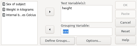 |
Screenshot 15.6: Using the Independent Sample T-test dialog, to test for differences of height between values of sex
In this case, the grouping variable is sex, so this is entered
as the variable for the GROUP subcommand. The group values are 0 (male) and
1 (female).
If you are running the proceedure using syntax, then you need to enter the values corresponding to each group within parentheses. If you are using the graphic user interface, then you have to open the “Define Groups” dialog box and enter the values corresponding to each group as shown in Screenshot 15.7. If, as in this case, the dataset has defined value labels for the group variable, then you can enter them by label or by value.
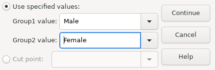 |
Screenshot 15.7: Setting the values of the grouping variable for an Independent Samples T-test
From Result 15.5, one can clearly see that the sample mean height is greater for males than for females. However in order to see if this is a significant result, one must consult the T-Test table.
The T-Test table contains two rows; one for use if the variance of the samples in each group may be safely assumed to be equal, and the second row if the variances in each group may not be safely assumed to be equal.
In this case however, both rows show a 2-tailed significance less than 0.001 and one must therefore reject the null hypothesis and conclude that within the population the mean height of males and of females are unequal.
| ||||||||||||||||||||||||||||||||||||||||||||||||||||||||||||||||
Result 15.5: The results of an independent samples T-test of height by sex