| [ < ] | [ > ] | [ << ] | [ Up ] | [ >> ] | [Top] | [Contents] | [Index] | [ ? ] |
| 6.1 Observation data and points | ||
| 6.2 Supported ellipsoids | ||
| 6.3 Transformation from spatial to geographical coordinates | ||
6.4 Class g3::Model |
| [ < ] | [ > ] | [ << ] | [ Up ] | [ >> ] | [Top] | [Contents] | [Index] | [ ? ] |
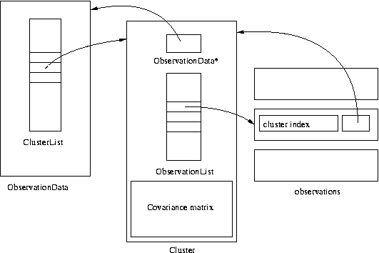
The Gama observation data structures are designed to enable adjustment of any combination of possibly correlated observations. At its very early stage Gama was limited to adjustment of uncorrelated observations. Only directions and distances were available and observable’s weight was stored together with the observed value in a single object. A single array of pointers to observation objects was sufficient for handling all observations. So called orientation shifts corresponding to directions measured form a point were stored together with coordinations in point objects.
To enable adjustment of possibly correlated observations (like angles
derived from observed directions or already adjusted coordinates from
a previous adjustment) Gama has come with the concept of
clusters. Cluster is an object with a common
variance-covariance matrix and a list of pointers to observation
objects (distances, directions, angles, etc.). Weights were removed
from observation objects and replaced with a pointer to the cluster to
which the observation belong. All clusters are joined in a common
object ObservationData; similarly to observations, each cluster
contains a pointer to its parent Observation Data object.
Orientation shifts were separated from coordinates and are
stored in the cluster containing the bunch of directions and thus
number of orientations is not limited to one for a point.
This organisation of observational information has proved to be
effective. Template classes ObservationData and Cluster
are used as base classes both in gama-local and gama-g3
template <typename Observation>
  class ObservationData
  {
  public:
    ClusterList<Observation>  CL;

    ObservationData();
    ObservationData(const ObservationData& cod);
    ~ObservationData();

    ObservationData& operator=(const ObservationData& cod);
    template <typename P> void for_each(const P& p) const;
  };

template <typename Observation>
  class Cluster
  {
  public:
    const ObservationData<Observation>*     observation_data;
    ObservationList<Observation>            observation_list;
    typename Observation::CovarianceMatrix  covariance_matrix;

    Cluster(const ObservationData<Observation>* od);
    virtual ~Cluster();

    virtual Cluster* clone(const ObservationData<Observation>*) const = 0;
    double stdDev(int i) const;
    int size() const;
    void update();
    int  activeCount() const;
    typename Observation::CovarianceMatrix activeCov() const;
  };
The following template class PointBase for handling point
information is used in gama-g3. The template class
PointBase relies internally on std::map container but
comes with its own interface (in gama-local std::map
was used directly for storing points).
template <typename Point>
  class PointBase
  {
    typedef std::map<typename Point::Name, Point*>  Points;

  public:
    PointBase();
    PointBase(const PointBase& cod);
    ~PointBase();

    PointBase& operator=(const PointBase& cod);
    void put(const Point&);
    void put(Point*);
    Point*       find(const typename Point::Name&);
    const Point* find(const typename Point::Name&) const;
    void erase(const typename Point::Name&);
    void erase();

    class const_iterator;
    const_iterator  begin();
    const_iterator  end  ();

    class iterator;
    iterator  begin();
    iterator  end  ();
  };
Template classes ObservationData and PointBase are
defined in namespace GNU_gama and are located in the source
directory gnu_gama.
| [ < ] | [ > ] | [ << ] | [ Up ] | [ >> ] | [Top] | [Contents] | [Index] | [ ? ] |
| id | a | b, 1/f, f | description | |
| airy | 6377563.396 | 6356256.910 | Airy ellipsoid 1830 | [4] |
| airy_mod | 6377340.189 | 6356034.446 | Modified Airy | [4] |
| apl1965 | 6378137 | 298.25 | Appl. Physics. 1965 | [4] |
| andrae1876 | 6377104.43 | 300.0 | Andrae 1876 (Denmark, Iceland) | [4] |
| australian | 6378160 | 298.25 | Australian National 1965 | [3] |
| bessel | 6377397.15508 | 6356078.96290 | Bessel ellipsoid 1841 | [1] |
| bessel_nam | 6377483.865 | 299.1528128 | Bessel 1841 (Namibia) | [4] |
| clarke1858a | 6378361 | 6356685 | Clarke ellipsoid 1858 1st | [3] |
| clarke1858b | 6378558 | 6355810 | Clarke ellipsoid 1858 2nd | [3] |
| clarke1866 | 6378206.4 | 6356583.8 | Clarke ellipsoid 1866 | [3] |
| clarke1880 | 6378316 | 6356582 | Clarke ellipsoid 1880 | [3] |
| clarke1880m | 6378249.145 | 293.4663 | Clarke ellipsoid 1880 (modified) | [4] |
| cpm1799 | 6375738.7 | 334.29 | Comm. des Poids et Mesures 1799 | [4] |
| delambre | 6376428 | 311.5 | Delambre 1810 (Belgium) | [4] |
| engelis | 6378136.05 | 298.2566 | Engelis 1985 | [4] |
| everest1830 | 6377276.345 | 300.8017 | Everest 1830 | [4] |
| everest1848 | 6377304.063 | 300.8017 | Everest 1948 | [4] |
| everest1856 | 6377301.243 | 300.8017 | Everest 1956 | [4] |
| everest1869 | 6377295.664 | 300.8017 | Everest 1969 | [4] |
| everest_ss | 6377298.556 | 300.8017 | Everest (Sabah and Sarawak) | [4] |
| fisher1960 | 6378166 | 298.3 | Fisher 1960 (Mercury Datum) | [3] [4] |
| fisher1960m | 6378155 | 298.3 | Modified Fisher 1960 | [3] [4] |
| fischer1968 | 6378150 | 298.3 | Fischer 1968 | [4] |
| grs67 | 6378160 | 298.2471674270 | GRS 67 (IUGG 1967) | [4] |
| grs80 | 6378137 | 298.257222101 | Geodetic Reference System 1980 | [1] |
| hayford | 6378388 | 297 | Hayford 1909 (International) | [1] [3] |
| helmert | 6378200 | 298.3 | Helmert ellipsoid 1906 | [3] |
| hough | 6378270 | 297 | Hough | [4] |
| iau76 | 6378140 | 298.257 | IAU 1976 | [4] |
| international | 6378388 | 297 | International 1924 (Hayford 1909) | [1] [3] |
| kaula | 6378163 | 298.24 | Kaula 1961 | [4] |
| krassovski | 6378245 | 298.3 | Krassovski ellipsoid 1940 | [1] |
| lerch | 6378139 | 298.257 | Lerch 1979 | [4] |
| mprts | 6397300 | 191.0 | Maupertius 1738 | [4] |
| mercury | 6378166 | 298.3 | Mercury spheroid 1960 | [3] |
| merit | 6378137 | 298.257 | MERIT 1983 | [4] |
| new_intl | 6378157.5 | 6356772.2 | New International 1967 | [4] |
| nwl1965 | 6378145 | 298.25 | Naval Weapons Lab., 1965 | [4] |
| plessis | 6376523 | 6355863 | Plessis 1817 (France) | [4] |
| se_asia | 6378155 | 6356773.3205 | Southeast Asia | [4] |
| sgs85 | 6378136 | 298.257 | Soviet Geodetic System 85 | [4] |
| schott | 6378157 | 304.5 | Schott 1900 spheroid | [3] |
| sa1969 | 6378160 | 298.25 | South American Spheroid 1969 | [3] |
| walbeck | 6376896 | 6355834.8467 | Walbeck | [4] |
| wgs60 | 6378165 | 298.3 | WGS 60 | [4] |
| wgs66 | 6378145 | 298.25 | WGS 66 | [4] |
| wgs72 | 6378135 | 298.26 | WGS 72 | [4] |
| wgs84 | 6378137 | 298.257223563 | World Geodetic System 1984 | [1] |
| [1] | Milos Cimbalnik - Leos Mervart: Vyssi geodezie 1, 1997, Vydavatelstvi CVUT, Praha |
| [2] | Milos Cimbalnik: Derived Geometrical Constants of the Geodetic Reference System 1980, Studia geoph. et geod. 35 (1991), pp. 133-144, NCSAV, Praha |
| [3] | Glossary of the Mapping Sciences, Prepared by a Joint Committe of the American Society of Civil Engineers, American Congress on Surveying and Mapping and American Society for Photogrammetry and Remote Sensing (1994), USA, ISBN 1-57083-011-8, ISBN 0-7844-0050-4 |
| [4] | Gerald Evenden: proj - forward cartographic projection filter (rel. 4.3.3), http://www.remotesensing.org/proj |
| [ < ] | [ > ] | [ << ] | [ Up ] | [ >> ] | [Top] | [Contents] | [Index] | [ ? ] |
Spatial coordinates (X, Y, Z) can be easily computed from geographical ellipsoidal coordinates (B, L, H), where B is geographical latitude, L geographical longitude and H is elliposidal height, as
X = (N + H) cos B cos L Y = (N + H) cos B sin L Z = (N(1-e^2) + H)sin B |
where N = a/sqrt(1 - e^2 sin^2 B) is the radius of curvature in the prime vertical, e^2 = (a^2 - b^2)/a^2 is the first eccentricity for the given rotational ellipsoid (spheroid) with semi-major axis a and semi-minor axis b.
In the case of coordiante transformation from (X, Y, Z) to (B, L, H), the longitude is given by the formula
tan L = Y / X. |
Now we can introduce
D = sqrt(X^2 + Y^2), |
so that the cartesian system become (D, Z). Coordinates B and H are then usually computed by iteration with some starting value of B_0, for example
tan B_0 = Z/D/(1 - e^2), |
tan B = Z/D + N/(N+H) e^2 tan B, H = D / cos B = Z / sin B - N(1-e^2) |
B. R. Bowring described a closed formula(3) that is more effective and sufficiantly accurate and that is used in GNU Gama.
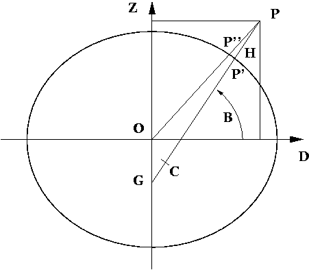
The centre of curvature C of the spheroid corresponding to P’ is the point
(e^2 a cos^3 u, -e’^2 b sin^3 u)),
where e’^2 = (a^2 - b^2)/b^2 is second eccentricity and u is the parametric latitude of the point P’, (1-e^2)N sin B = b sin u. Therefore
tan B = (Z + e’^2 b sin^3 u) / (D - e^2 a cos^3 u).
This is clearly an iterative solution; but it has been found that this formula is extremely accurate using the single first approximation for u for the tan u = (Z/D)(a/b). Maximum error in earth bound region is 3e-8 of sexagesimal arc seconds (5e-7 millimetres); maximum is 0.0018” (0.1 millimetres) at height H = 2a.
| [ < ] | [ > ] | [ << ] | [ Up ] | [ >> ] | [Top] | [Contents] | [Index] | [ ? ] |
g3::Modelg3::model documentation shall come here ...
namespace GNU_gama {  namespace g3 {


  class Model {
  public:

    typedef GNU_gama::PointBase<g3::Point>              PointBase;
    typedef GNU_gama::ObservationData<g3::Observation>  ObservationData;

    PointBase           *points;
    ObservationData     *obs;

    GNU_gama::Ellipsoid  ellipsoid;


    Model();
    ~Model();

    Point* get_point(const Point::Name&);
    void   write_xml(std::ostream& out) const;
    void   pre_linearization();
}}
| [ << ] | [ >> ] | [Top] | [Contents] | [Index] | [ ? ] |
This document was generated on February 17, 2024 using texi2html 1.82.