5. Network adjustment with gama-local

Adjustment of local geodetic network is a classical case of adjustment of indirect observations. After estimation of approximate values of unknown parameters (coordinates of points) and linearization of functions describing relations between observations and parameters we solve linear system of equations

(1)      Ax = b + v,

where A is coefficient matrix, b is vector of absolute terms (right hand side) and v is vector of residuals. This system is (generally) overdetermined and we seek the solution x satisfying the basic criterion of Least Squares

(2)      v'Pv = min,

where P is weight matrix. This criterion unambiguously defines the shape of adjusted network.

Geodetic adjustment is traditionally computed as the solution of normal equations (2)

(a)      Nx = n,  where  N=A'PA  and  n=A'Pb.

In the case of free network, i.e. network with no fixed coordinates (or network without sufficient number of fixed coordinates), the system (1) is singular, matrix A has linearly dependent columns, and there is infinite number of solutions x.

To define a unique solution x we need to definine a set of constriant equations (inner constraints)

(b)      Cx = c

to minimize

(c)      v'Pv - 2k'(Cx - c) = min

where r is the vector of residuals, r = Ax - b, k is a vector of so called Lagrange multipliers and adjusted vector x is obtained from solution of

(d)      ( A'PA, C') (x) = (A'Pb)
         ( C,    0 ) (k) = (  c )

In gama-local a slightly different approach is used, we define a second regularization criterion as

(3)      \sum x_i^2 = min,      for all selected i

stating that at the same time with (2) we demand that the sum of squares corrections of selected parameters is minimal (corrections of unknown parameters with indexes from the set of all selected unknowns. Geometrically this criterion is equivalent to adjustment of the network according to (2) with simultaneous transformation to the selected set of fiducial points. This transformation does not change the shape of adjusted network.

Often it is advantageous to work with a homogenized system, ie. with the system of project equations in which coefficient of each row and absolute term are multiplied by square root of the weight of corresponding observation.

(4)      ~A x = ~b,

where ~A = P^1/2 A, ~b = P^1/2 A. Symbol P^1/2 denotes diagonal matrix of square roots of observation weights (or Cholesky decomposition of covariance matrix in the case of correlated observations). To criterion (2) corresponds in the case of homogenized system criterion

(5)      ~v'~v = min.

Normal equations are clearly equivalent for both systems.

5.1 Approximate coordinates

For computation of coefficients in system (1) (ie. during linearization) we need, first of all, an estimate of approximate coordinates of points and approximate values of orientations of observed directions sets.

Approximate values of unknown parameters are usually not known and we have to compute them from the available observations. For approximate value of orientation program gama-local uses median of all estimates from the given set of directions to the points with known coordinates. Median is less sensitive to outliers than arithmetic mean which is normally used for approximate estimate of orientations

During the phase of computation of approximate coordinate of points, program gama-local walks through the list of computed points and for each point gathers all determining elements pointing to points with known or previously computed coordinates. Determining elements are

• outer bearing (oriented half-line) starting from the point with known coordinates and pointing to the computed point

  distance between given and computed points

• inner angle with vertex in the computed point and arms intersecting given points

For all combinations of determining elements program gama-local computes intersections and estimates approximate coordinates as the median of all available solutions.

If at least one point was resolved while iterating through the list, the whole cycle is repeated.

If no more coordinates can be solved using intersections and points with unknown coordinates are remaining, program tries to compute coordinates of unresolved points in a local coordinates system and obtain their coordinates using similarity transformation. If a transformation succeeds to resolve coordinates at least one computed point and there are still some points without coordinates left, the whole process is repeated. Classes for computation of approximate coordinates have been written by Jiri Vesely.

If program gama-local fails to compute approximate coordinates of some of the network points, they are eliminated from the adjustment and they are listed in the output listing.

With the outlined strategy, program gama-local is able to estimate approximate coordinates in most of the cases we normally meet in surveying profession. Still there are cases in which the solution fails. One example is an inserted horizontal traverse with sets of observed direction on both ends but without a connecting observed distance. The solution of approximate coordinates can fail when there is a number of gross error for example resulting from confusion of point identifications but in normal situations, leaving computation of approximate coordinates on program gama-local is recommended.

Example

Computation of approximate coordinates of points
************************************************

Number of points with given coordinates:      2
Number of solved points                :      2
Number of observations                 :      4
-----------------------------------------------------
Successfully solved points             :      0
Remaining unsolved points              :      2


List of unresolved points
*************************
422
424

5.2 Gross absolute terms

One of parameters in XML input of program gama-local is tolerance tol-abs for detecting of gross absolute terms in project equations. Observations with outlying absolute terms are always excluded from adjustment.

For measured distances program tests difference between observed value d_i and distance computed from approximate coordinates d_0

         |d_i - d_0| > tol-abs,

for observed directions program gama-local tests transverse deviation corresponding to absolute term b_i from project equations (1)

         | b_i | d_0 > tol-abs

and similarly for angles, program tests the greater of two deviations corresponding to left and right distances (left and right arm of the angle)

         |b_i| max{ d_{0_l}, d_{0_r} }  > tol-abs.

Default value of parameter tol-abs is 1000 mm.

Example

Outlying absolute terms in project equations
********************************************

   i   standpoint       target           observed     absolute
=========================================== value ===== term ==

   2          103          104 dir.    301.087900       -9989.1


Observations with outlying absolute terms removed

5.3 Parameters of statistical analysis

Program gama-local uses two basic statistical parameters

• confidence probability P (default value is 95%, see input XML parameter conf-pr) and
• actual type of reference standard deviation m0_a (parameter sigma-act).

Confidence probability determines significance level on which statistical tests of adjusted quantities are carried. Actual type of reference standard deviation m0_a specifies whether during statistical analysis we use an a priori reference standard deviation m0 or an a posteriori estimate m0’. On the type of actual reference standard deviation depends the choice of density functions of stochastic quantities in statistical analysis of the adjustment.

• A priori reference standard deviation m0 is an estimate of the standard deviation of an observation with the unit weight. Numerically it is a scaling factor used in calculation of the weights. If we change m0, only the sum of weighted residuals squares is changed and all adjustment results remain the same (there is just one least squares solution). m0 can be selected in cases when we know its value in advance and with sufficient reliability. Another situation when m0 is used are networks with low number of degrees of freedom (poorly overdetermined systems) or when veen degrees of freedom is zero. Examples may be analysis of network models etc.
• A posteri estimate of reference standard deviation m0’ is used in cases when a priori value of reference standard deviation m0 is not known and when degrees of freedom is sufficiently high and reliable for empirical estimate of m0’.

The standard deviantion of an adjusted quantity is computed in dependence of the choice of actual type of reference standard deviation m0_a according to formula

m0_a sqrt(q)

where q is the weight coefficient of the corresponding adjusted unknown parameter or observation. Apart from the standard deviation, program gama-local computes for the adjusted quantity its confidence interval in which its real value is located with the probabilityP.

5.4 Test on the reference standard deviation

Null hypothesis H_0: m0 = m0’ is tested versus alternative hypothesis H_1: m0 neq m0’. Test criterion is ratio of a posteriori estimate of reference standard deviation

         m0' = sqrt( v'P v / r).

and a priori reference standard deviation m0 (input data parameter m0-apr). For given significance level alpha lower and upper bounds of interval (L, U) are computed so, that if hypothesis H_0 is true, probabilities P(m0’/m0 le D) and P(m0’/m0 ge H) are equal to alpha/2. Lower and upper bounds of the interval are computed as

         L = sqrt((Chi^2_{1-alpha/2,r})/r),
         U = sqrt((Chi^2_{ alpha/2 ,r})/r).

Probability

         P(L < m0'/m0 < U) = conf-pr

is by default 95%, this corresponds to 5% confidence level test.

Exceeding the upper limit H of the confidence interval can be caused even by a single gross error (one outlying observation). Method of Least Squares is generally very sensitive to presence of outliers. Safely can be detected only one observation whose elimination leads to maximal decrease of a posteriori estimate of reference standard deviation

(6)      m0''  = sqrt{(v'P v - delta)/(r-1)},
         delta = max(v_i^2/q_vi),

where

(7)      q_vi = 1/p_i - q_Li

is weight coefficient of i-th residual. If the set of observations contains only one gross error, the outlying observation is likely to be detected, but this can not be guaranteed.

In addition, program gama-local computes a posteriori estimate of reference standard deviation separately for horizontal distances and directions and/or angles after formula from

         m0'_t = sqrt(sum{~v^2_it}) / sum{~q_vi}),    t=d,s,

where symbol t denotes observed distances, directions and/or angles.

Example

m0  apriori  :    10.00
m0' empirical:     9.64         [pvv] : 3.43560e+03

During statistical analysis we work

- with empirical standard deviation 9.64
- with confidence level             95 %

Ratio m0' empirical / m0 apriori: 0.964
95 % interval (0.773, 1.227) contains value m0'/m0
m0'/m0 (distances): 0.997   m0'/m0 (directions): 0.943

Maximal decrease of m0''/m0 on elimination of one observation: 0.892

Maximal studentized residual 2.48 exceeds critical value 1.95
on significance level 5 % for observation #35
<distance from="407" to="422" val="346.415" stdev="5.0" />

5.5 Information on points

Program gama-local lists separately review of coordinates of fixed and adjusted points; adjusted constrained coordinates are marked with *; see equation (3). Adjusted coordinate standard deviations m_x and m_y, and values for computing confidence intervals are given in the listing of adjusted coordinates (Parameters of statistical analysis). In the review index i is the index of unknown x_i from the system of project equations (1) corresponding to the point coordinates x and y.

Example

Fixed points
************

       point         x              y
========================================

           1  1054980.484     644498.590
           2  1054933.801     643654.101


Adjusted coordinates
********************

  i        point    approximate  correction  adjusted    std.dev conf.i.
====================== value ====== [m] ====== value ========== [mm] ===

             422
  2            x   1055167.22747  -0.00510 1055167.22237     2.7     5.4
  3            y    644041.46119   0.00023  644041.46142     2.5     5.1

             424
  4            X * 1055205.41198  -0.00056 1055205.41142     3.1     6.3
  5            Y *  644318.24425  -0.00125  644318.24300     3.6     7.2

For adjusted points, program summarizes information on standard ellipses, confidence ellipses, mean square positional errors (m_p), mean coordinate errors (m_xy) and coefficients g characterizing position of approximate coordinates with regard to the confidence ellipse.

Example

Mean errors and parameters of error ellipses
********************************************

  point     mp      mxy      mean error ellipse  conf.err. ellipse   g
========== [mm] == [mm] ==== a [mm] b  alpha[g] ==== a' [mm] b' ========

    422     3.6     2.6     2.7     2.5   187.0     6.8     6.4     0.8
    424     4.7     3.4     3.7     2.9   131.8     9.5     7.4     0.2
    403     5.7     4.0     4.3     3.6    78.9    11.0     9.3     1.1

Mean square positional error m_p and mean coordinate error (m_xy) are computed as

         m_p = sqrt(m_y^2 + m_x^2),    m_xy = m_p / sqrt(2),

where m_y^2 and m_x^2 are squares of standard deviations (variances) of adjusted points coordinates.

Semimajor and semiminor axes of standard ellipse are denoted as a and b in the listing, bearing of semimajor axis is denoted as alpha and they are computed from covariances of adjusted coordinates

         a = sqrt(1/2(cov_yy + cov_xx + c),
         b = sqrt(1/2(cov_yy + cov_xx - c),

         c = sqrt( (cov_xx - cov_yy)^2 + 4(cov_xy)^2 ),

         tan 2alpha = 2(cov_xy) / (cov_xx - cov_yy).

The angle alpha (the bearing of semimajor axis) is measured clockwise from X axis.

Probability that standard ellipse covers real position of a point is relatively low. For this reason program gama-local computes extra confidence ellipse for which the probability of covering real point position is equal to the given confidence probability. Both ellipses are located in the same center, they share the same bearing of semimajor axes and they are similar. For lengths of their semi-axis holds

         a' = k_p a,        b' = k_p b,

where k_p is a coefficient computed for the given probability P as defined in Parameters of statistical analysis.

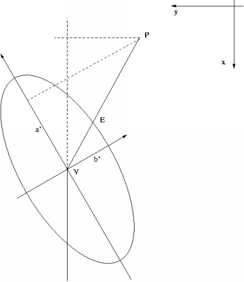
Position of approximate coordinates of an adjusted point with respect to its confidence ellipse are expressed by a coeeficient g Three cases are possible

• g < 1 approximate coordinates of adjusted point are located inside the confidence ellipse
• g = 1 approximate coordinates of adjusted point are located on the confidence ellipse
• g > 1 approximate coordinates of adjusted point are outside the confidence ellipse

The coefficient g is calculated from formula

         g = sqrt( (a_0 / a')^2 + (b_0/b')^2 )

where

         b_0 = delta_y cos(alpha) - delta_x sin(alpha),
         a_0 = delta_y sin(alpha) - delta_x cos(alpha)

symbol delta is used for correction of approximate coordinates and alpha is bearing of confidence ellipse semimajor axis.

If network contains sets of observed directions, program writes information on corresponding adjusted orientations, standard deviations and confidence intervals. Index i is the same as in the case of adjusted coordinates the index of i-th adjusted unknown in the project equations.

Example

Adjusted bearings
*****************

  i   standpoint   approximate  correction  adjusted   std.dev conf.i.
==================== value [g] ==== [g] === value [g] ======= [cc] ===

  1            1    296.484371  -0.000917  296.483454      5.1    10.3
 10            2     96.484371   0.000708   96.485079      5.1    10.4
 21          403     20.850571  -0.001953   20.848618      8.8    17.7

5.6 Adjusted observations and residuals

In the review of adjusted observations program gama-local prints index of the observation, index of the row in matrix A in the system (1), identifications of standpoint and target point, type of the observation, its approximate and adjusted value, standard deviation and confidence interval.

Example

Adjusted observations
*********************

   i   standpoint   target         observed     adjusted std.dev conf.i.
===================================== value ==== [m|g] ====== [mm|cc] ==

   1            1        2 dis.   845.77700    845.77907     3.0     6.1
   2                   422 dir.   28.205700    28.205613     5.1    10.3
   3                   424 dir.   60.490600    60.491359     6.7    13.6

Review of residuals serves for analysis of observations and containts values of normalized or studentized residuals (depending on type of m0_a used) and three characteristics. Theese are coefficient f identifying weak network elements and estimates of real error of observation e-obs and real error of its adjusted value e-adj, see definition in the following text.

If normalized or studentized residual exceeds critical value for the given confidence probability, it is marked in the review with symbol c (critical) and maximal normalized or studentized residual is marked with symbol m.

Example

Residuals and analysis of observations
**************************************

   i standpoint   target        f[%]        v    |v'|     e-obs.  e-adj.
======================================== [mm|cc] =========== [mm|cc] ===

   1          1        2 dir.   47.4       9.170  1.1      12.7    3.5
   2                 422 dir.   47.0      -0.873  0.1      -1.2   -0.3
   3                 424 dir.   30.3       7.588  1.1      14.8    7.2

5.7 Identification of weak network elements

When planning observations in a geodetic network we always try to guarantee that all observed elements are checked by other measurements. Only with redundant measurements it is possible to adjust observations and possibly remove blunders that might otherwise totaly corrupt the whole set of measurements. Apart from sufficient number of redundant observations the degree of control of single observed elements is given by the network configuration, ie. its geometry.

Less controlled observations represent weak network elements and they can in extreme cases even disable detection of gross observational errors as it is in the case of uncontrolled observations. There are two limit cases of observation control

• fully controlled observation as is for example an observed distance between two fixed points (standard deviation of the adjusted element is zero; standard deviation of the residual equals to the standard deviation if the observation) and
• uncontrolled observations as is a free polar bar for example (standard deviation of adjusted value is equal to standard deviation of observed quantity; residual and standard deviation of the residual are zero).

Weakly controlled or uncontrolled observations can result even from elimination of certain suspisios observations during analysis of adjusment.

Standard deviation of adjusted observations is less than standard deviation of the measurement. Degree of observation control in network is defined as coefficient

(8)      f = 100 (m_l - m_L)/m_l,

where m_l is standard deviation of observed quantity and m_L is standard deviation computed from a posteriori reference standard deviation m0. We consider observed network element to be

• uncontrolled if f < 0.1 (in listing marked with letter u),
• weakly controlled if 0.1 le f < 5 (in listing marked with letter w).

5.8 Estimation of real errors

Acording to previous section we can consider an observation to be controlled if its coefficient f > 0.1. Any controlled observation can be eliminated from the network without corrupting the network consistency—network reduced by one controlled observation can be adjusted and all unknown parameters can be compute without the eliminated observation.

Estimate of real error of i-th observation is defined as

(9)      e_li = L^red_i - l_i,

where e_li is value of i-th observation and is value of i-th network element computed from adjusted coordinates and/or orientations of the reduced network. Similarly is defined the estimate of real error of a residual

(10)     e_vi = L^red_i - L_l.

Adjustment results are the best statistical estimate of unknown parameters that we have. This holds true even for adjustment of reduced network which is not influenced by real error of i-th observation. On favourable occasions differences (9) and (10) can help to detect blunders but to interpret these estimates as real errors is possible only with substantial exaggeration. These estimates fail when there are more than one significant observational error. Generally holds tha the weaker the element is controlled in netowrk the less reliable these estimates are.

Estimate of real error of an observation computes program gama-local as

         e_li = v_i/(p_i q_vi)

and estimate of real error of a residual as

         e_vi = e_li - v_i.

5.9 Test on linearization

Mathematical model of geodetic network adjustment in gama-local is defined as a set of known real-valued differentiable functions

(11)      L^* = f(X^*)

where L^* is a vector of theoretical correct observations and X^* is a vector of correct values of parameters. For the given sample set of observations L and the unknown vector of residuals v we can express the estimate of parameters X as a nonlinear set of equations

(12)      L + v = f(X).

With approximate values X_0 of unknown parameters

(12)      X = X_0 + x

we can linearize the equations (12)

          L + v = f(X_0) + f'(X_0)x.

yielding the linear set of equations (1)

Unknown parameters in gama-local mathematical model are points coordinates and orientation angles (transforming observed directions to bearings). The observables described by functions (12) belong into two classes

• linear observables: horizontal and slope distances, height differences, control coordinates and vectors (coordinate differences),
• angular observables: directions, horizontal and zenith angles.

Internally in gama-local unknown corrections to linear observables are computed in millimeters and corrections to angular observables in centigrade seconds. To reflect the internal units in used all partial derivatives of angular observables by coordinates are scaled by factor 2000/pi.

When computing coefficients of project equations (1) we expect that approximate coordinates of points are known with sufficient accuracy needed for linearization of generally nonlinear relations between observations and unknown paramters. Most often this is true but not always and generally we have to check how close our approximation is to adjusted parameters.

Generally we check linearization in adjustment by double calculation of residuals

         v^I  = Ax - b,
         v^II = ~l(~x) - l,

Program gama-local similarly computes and tests differences in values of adjusted observations once computed from residuals and once from adjusted coordinates. For measured directions and angles gama-local computes in addition transverse deviation corresponding to computed angle difference in the distance of target point (or the farther of two targets for angle). As a criterion of bad linearization is supposed positional deviation greater or equal to 0.0005 millimetres.

Example

Test of linearization error
***************************

Diffs in adj. obs from residuals and from adjusted coordinates
**************************************************************

 i standpoint     target          observed     r        difference
=================================   value  = [mm|cc] = [cc] == [mm]=

 2 3022184030 3022724008 dist.   28.39200    -7.070          -0.003
 3            3022724002 dist.   72.30700   -18.815          -0.001
 7            3000001063 dir.  286.305200    11.272  -0.002  -0.001
 8            3022724008 dir.  357.800600   -23.947   0.037   0.002

From the practical point of view it might seem that the tolerance 0.0005 mm for detecting poor linearization is too strict. Its exceeding in program gama-local results in repeated adjustment with substitute adjusted coordinates for approximate. Given tolerance was chosen so strict to guarantee that listed output results would never be influenced by linearization and could serve for verification and testing of numerical solutions produced by other programs.

Iterated adjustement with successive improvement of approximate unknown coordinates converges usually even for gross errors in initial estimates of unknown coordinates. If the influence of linearization is detected after adjustment, typically only one iteration is sufficient for recovering.

For any automatically controlled iteration we have to set up certain stopping criterion independent on the convergence and results obtained. Program gama-local computes iterated adjustment three times at maximum. If the bad linearization is detected even after three readjustments it signals that given network configuration is somehow suspicious.

5.10 Glossary

Symbols and names used in adjustment statistics.

This document was generated on February 17, 2024 using texi2html 1.82.