28.5 Polynomial Interpolation 
Octave comes with good support for various kinds of interpolation,
most of which are described in Interpolation. One simple alternative
to the functions described in the aforementioned chapter, is to fit
a single polynomial, or a piecewise polynomial (spline) to some given
data points. To avoid a highly fluctuating polynomial, one most often
wants to fit a low-order polynomial to data. This usually means that it
is necessary to fit the polynomial in a least-squares sense, which just
is what the polyfit function does.
- :
p =polyfit(x, y, n)¶ - :
[p, s] =polyfit(x, y, n)¶ - :
[p, s, mu] =polyfit(x, y, n)¶ Return the coefficients of a polynomial p(x) of degree n that minimizes the least-squares-error of the fit to the points
[x(:), y(:)].n is typically an integer ≥ 0 specifying the degree of the approximating polynomial. If n is a logical vector, it is used as a mask to selectively force the corresponding polynomial coefficients to be used or ignored.
The polynomial coefficients are returned in the row vector p. The output p may be directly used with
polyvalto estimate values using the fitted polynomial.The optional output s is a structure containing the following fields:
- ‘yf’
The values of the polynomial for each value of x.
- ‘X’
The Vandermonde matrix used to compute the polynomial coefficients.
- ‘R’
Triangular factor R from the QR decomposition.
- ‘C’
The unscaled covariance matrix, formally equal to the inverse of x’*x, but computed in a way minimizing roundoff error propagation.
- ‘df’
The degrees of freedom.
- ‘normr’
The norm of the residuals.
The second output may be used by
polyvalto calculate the statistical error limits of the predicted values. In particular, the standard deviation of p coefficients is given bysqrt (diag (s.C)/s.df) * s.normr.When the third output, mu, is present the original data is centered and scaled which can improve the numerical stability of the fit. The coefficients p are associated with a polynomial in
xhat = (x - mu(1)) / mu(2)
where mu(1) = mean (x), and mu(2) = std (x).Example 1 : logical n and integer n
f = @(x) x.^2 + 5;   # data-generating function
x = 0:5;
y = f (x);
## Fit data to polynomial A*x^3 + B*x^1
p = polyfit (x, y, logical ([1, 0, 1, 0]))
⇒ p = [ 0.0680, 0, 4.2444, 0 ]
## Fit data to polynomial using all terms up to x^3
p = polyfit (x, y, 3)
⇒ p = [ -4.9608e-17, 1.0000e+00, -3.3813e-15, 5.0000e+00 ]
See also: polyval, polyaffine, roots, vander, zscore.
In situations where a single polynomial isn’t good enough, a solution
is to use several polynomials pieced together. The function
splinefit fits a piecewise polynomial (spline) to a set of
data.
- :
pp =splinefit(x, y, breaks)¶ - :
pp =splinefit(x, y, p)¶ - :
pp =splinefit(…, "periodic", periodic)¶ - :
pp =splinefit(…, "robust", robust)¶ - :
pp =splinefit(…, "beta", beta)¶ - :
pp =splinefit(…, "order", order)¶ - :
pp =splinefit(…, "constraints", constraints)¶ -
Fit a piecewise cubic spline with breaks (knots) breaks to the noisy data, x and y.
x is a vector, and y is a vector or N-D array. If y is an N-D array, then x(j) is matched to y(:,…,:,j).
p is a positive integer defining the number of intervals along x, and p+1 is the number of breaks. The number of points in each interval differ by no more than 1.
The optional property periodic is a logical value which specifies whether a periodic boundary condition is applied to the spline. The length of the period is
max (breaks) - min (breaks). The default value isfalse.The optional property robust is a logical value which specifies if robust fitting is to be applied to reduce the influence of outlying data points. Three iterations of weighted least squares are performed. Weights are computed from previous residuals. The sensitivity of outlier identification is controlled by the property beta. The value of beta is restricted to the range, 0 < beta < 1. The default value is beta = 1/2. Values close to 0 give all data equal weighting. Increasing values of beta reduce the influence of outlying data. Values close to unity may cause instability or rank deficiency.
The fitted spline is returned as a piecewise polynomial, pp, and may be evaluated using
ppval.The splines are constructed of polynomials with degree order. The default is a cubic, order=3. A spline with P pieces has P+order degrees of freedom. With periodic boundary conditions the degrees of freedom are reduced to P.
The optional property, constraints, is a structure specifying linear constraints on the fit. The structure has three fields,
"xc","yc", and"cc"."xc"Vector of the x-locations of the constraints.
"yc"Constraining values at the locations xc. The default is an array of zeros.
"cc"Coefficients (matrix). The default is an array of ones. The number of rows is limited to the order of the piecewise polynomials, order.
Constraints are linear combinations of derivatives of order 0 to order-1 according to
cc(1,j) * y(xc(j)) + cc(2,j) * y'(xc(j)) + ... = yc(:,...,:,j).
See also: interp1, unmkpp, ppval, spline, pchip, ppder, ppint, ppjumps.
The number of breaks (or knots) used to construct the piecewise polynomial is a significant factor in suppressing the noise present in the input data, x and y. This is demonstrated by the example below.
x = 2 * pi * rand (1, 200);
y = sin (x) + sin (2 * x) + 0.2 * randn (size (x));
## Uniform breaks
breaks = linspace (0, 2 * pi, 41); % 41 breaks, 40 pieces
pp1 = splinefit (x, y, breaks);
## Breaks interpolated from data
pp2 = splinefit (x, y, 10);  % 11 breaks, 10 pieces
## Plot
xx = linspace (0, 2 * pi, 400);
y1 = ppval (pp1, xx);
y2 = ppval (pp2, xx);
plot (x, y, ".", xx, [y1; y2])
axis tight
ylim auto
legend ({"data", "41 breaks, 40 pieces", "11 breaks, 10 pieces"})
The result of which can be seen in Figure 28.1.
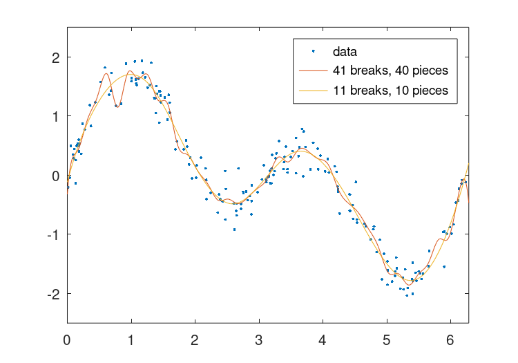
Figure 28.1: Comparison of a fitting a piecewise polynomial with 41 breaks to one with 11 breaks. The fit with the large number of breaks exhibits a fast ripple that is not present in the underlying function.
The piecewise polynomial fit, provided by splinefit, has
continuous derivatives up to the order-1. For example, a cubic fit
has continuous first and second derivatives. This is demonstrated by
the code
## Data (200 points)
x = 2 * pi * rand (1, 200);
y = sin (x) + sin (2 * x) + 0.1 * randn (size (x));
## Piecewise constant
pp1 = splinefit (x, y, 8, "order", 0);
## Piecewise linear
pp2 = splinefit (x, y, 8, "order", 1);
## Piecewise quadratic
pp3 = splinefit (x, y, 8, "order", 2);
## Piecewise cubic
pp4 = splinefit (x, y, 8, "order", 3);
## Piecewise quartic
pp5 = splinefit (x, y, 8, "order", 4);
## Plot
xx = linspace (0, 2 * pi, 400);
y1 = ppval (pp1, xx);
y2 = ppval (pp2, xx);
y3 = ppval (pp3, xx);
y4 = ppval (pp4, xx);
y5 = ppval (pp5, xx);
plot (x, y, ".", xx, [y1; y2; y3; y4; y5])
axis tight
ylim auto
legend ({"data", "order 0", "order 1", "order 2", "order 3", "order 4"})
The result of which can be seen in Figure 28.2.
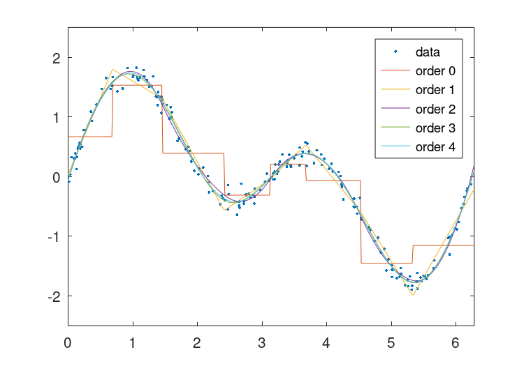
Figure 28.2: Comparison of a piecewise constant, linear, quadratic, cubic, and quartic polynomials with 8 breaks to noisy data. The higher order solutions more accurately represent the underlying function, but come with the expense of computational complexity.
When the underlying function to provide a fit to is periodic, splinefit
is able to apply the boundary conditions needed to manifest a periodic fit.
This is demonstrated by the code below.
## Data (100 points)
x = 2 * pi * [0, (rand (1, 98)), 1];
y = sin (x) - cos (2 * x) + 0.2 * randn (size (x));
## No constraints
pp1 = splinefit (x, y, 10, "order", 5);
## Periodic boundaries
pp2 = splinefit (x, y, 10, "order", 5, "periodic", true);
## Plot
xx = linspace (0, 2 * pi, 400);
y1 = ppval (pp1, xx);
y2 = ppval (pp2, xx);
plot (x, y, ".", xx, [y1; y2])
axis tight
ylim auto
legend ({"data", "no constraints", "periodic"})
The result of which can be seen in Figure 28.3.
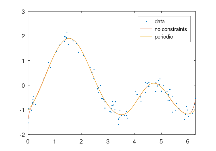
Figure 28.3: Comparison of piecewise polynomial fits to a noisy periodic function with, and without, periodic boundary conditions.
More complex constraints may be added as well. For example, the code below illustrates a periodic fit with values that have been clamped at the endpoints, and a second periodic fit which is hinged at the endpoints.
## Data (200 points)
x = 2 * pi * rand (1, 200);
y = sin (2 * x) + 0.1 * randn (size (x));
## Breaks
breaks = linspace (0, 2 * pi, 10);
## Clamped endpoints, y = y' = 0
xc = [0, 0, 2*pi, 2*pi];
cc = [(eye (2)), (eye (2))];
con = struct ("xc", xc, "cc", cc);
pp1 = splinefit (x, y, breaks, "constraints", con);
## Hinged periodic endpoints, y = 0
con = struct ("xc", 0);
pp2 = splinefit (x, y, breaks, "constraints", con, "periodic", true);
## Plot
xx = linspace (0, 2 * pi, 400);
y1 = ppval (pp1, xx);
y2 = ppval (pp2, xx);
plot (x, y, ".", xx, [y1; y2])
axis tight
ylim auto
legend ({"data", "clamped", "hinged periodic"})
The result of which can be seen in Figure 28.4.
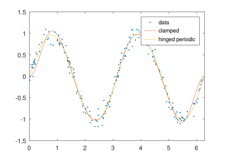
Figure 28.4: Comparison of two periodic piecewise cubic fits to a noisy periodic signal. One fit has its endpoints clamped and the second has its endpoints hinged.
The splinefit function also provides the convenience of a robust
fitting, where the effect of outlying data is reduced. In the example below,
three different fits are provided. Two with differing levels of outlier
suppression and a third illustrating the non-robust solution.
## Data
x = linspace (0, 2*pi, 200);
y = sin (x) + sin (2 * x) + 0.05 * randn (size (x));
## Add outliers
x = [x, linspace(0,2*pi,60)];
y = [y, -ones(1,60)];
## Fit splines with hinged conditions
con = struct ("xc", [0, 2*pi]);
## Robust fitting, beta = 0.25
pp1 = splinefit (x, y, 8, "constraints", con, "beta", 0.25);
## Robust fitting, beta = 0.75
pp2 = splinefit (x, y, 8, "constraints", con, "beta", 0.75);
## No robust fitting
pp3 = splinefit (x, y, 8, "constraints", con);
## Plot
xx = linspace (0, 2*pi, 400);
y1 = ppval (pp1, xx);
y2 = ppval (pp2, xx);
y3 = ppval (pp3, xx);
plot (x, y, ".", xx, [y1; y2; y3])
legend ({"data with outliers","robust, beta = 0.25", ...
         "robust, beta = 0.75", "no robust fitting"})
axis tight
ylim auto
The result of which can be seen in Figure 28.5.
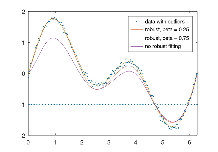
Figure 28.5: Comparison of two different levels of robust fitting (beta = 0.25 and 0.75) to noisy data combined with outlying data. A conventional fit, without robust fitting (beta = 0) is also included.
A very specific form of polynomial interpretation is the Padé approximant. For control systems, a continuous-time delay can be modeled very simply with the approximant.
- :
[num, den] =padecoef(T)¶ - :
[num, den] =padecoef(T, N)¶ Compute the Nth-order Padé approximant of the continuous-time delay T in transfer function form.
The Padé approximant of
exp (-sT)is defined by the following equationPn(s) exp (-sT) ~ ------- Qn(s)Where both Pn(s) and Qn(s) are Nth-order rational functions defined by the following expressions
         N    (2N - k)!N!        k
Pn(s) = SUM --------------- (-sT)
        k=0 (2N)!k!(N - k)!

Qn(s) = Pn(-s)
The inputs T and N must be non-negative numeric scalars. If N is unspecified it defaults to 1.
The output row vectors num and den contain the numerator and denominator coefficients in descending powers of s. Both are Nth-order polynomials.
For example:
t = 0.1;
n = 4;
[num, den] = padecoef (t, n)
⇒ num =

      1.0000e-04  -2.0000e-02   1.8000e+00  -8.4000e+01   1.6800e+03

⇒ den =

      1.0000e-04   2.0000e-02   1.8000e+00   8.4000e+01   1.6800e+03
The function, ppval, evaluates the piecewise polynomials, created
by mkpp or other means, and unmkpp returns detailed
information about the piecewise polynomial.
The following example shows how to combine two linear functions and a quadratic into one function. Each of these functions is expressed on adjoined intervals.
x = [-2, -1, 1, 2];
p = [ 0,  1, 0;
      1, -2, 1;
      0, -1, 1 ];
pp = mkpp (x, p);
xi = linspace (-2, 2, 50);
yi = ppval (pp, xi);
plot (xi, yi);
- :
pp =mkpp(breaks, coefs)¶ - :
pp =mkpp(breaks, coefs, d)¶ -
Construct a piecewise polynomial (pp) structure from sample points breaks and coefficients coefs.
breaks must be a vector of strictly increasing values. The number of intervals is given by
ni = length (breaks) - 1.When m is the polynomial order coefs must be of size: ni-by-(m + 1).
The i-th row of coefs,
coefs(i,:), contains the coefficients for the polynomial over the i-th interval, ordered from highest (m) to lowest (0) degree.coefs may also be a multi-dimensional array, specifying a vector-valued or array-valued polynomial. In that case the polynomial order m is defined by the length of the last dimension of coefs. The size of first dimension(s) are given by the scalar or vector d. If d is not given it is set to
1. In this casep(r, i, :)contains the coefficients for the r-th polynomial defined on interval i. In any case coefs is reshaped to a 2-D matrix of size[ni*prod(d) m].Programming Note:
ppvalevaluates polynomials atxi - breaks(i), i.e., it subtracts the lower endpoint of the current interval from xi. This must be taken into account when creating piecewise polynomials objects withmkpp.See also: unmkpp, ppval, spline, pchip, ppder, ppint, ppjumps.
- :
[x, p, n, k, d] =unmkpp(pp)¶ -
Extract the components of a piecewise polynomial structure pp.
This function is the inverse of
mkpp: it extracts the inputs tomkppneeded to create the piecewise polynomial structure pp. The code below makes this relation explicit:[breaks, coefs, numinter, order, dim] = unmkpp (pp); pp2 = mkpp (breaks, coefs, dim);
The piecewise polynomial structure
pp2obtained in this way, is identical to the originalpp. The same can be obtained by directly accessing the fields of the structurepp.The components are:
- x
Sample points or breaks.
- p
Polynomial coefficients for points in sample interval.
p(i, :)contains the coefficients for the polynomial over interval i ordered from highest to lowest degree. Ifd > 1, then p is a matrix of size[n*prod(d) m], where thei + (1:d)rows are the coefficients of all the d polynomials in the interval i.- n
Number of polynomial pieces or intervals,
n = length (x) - 1.- k
Order of the polynomial plus 1.
- d
Number of polynomials defined for each interval.
- :
yi =ppval(pp, xi)¶ Evaluate the piecewise polynomial structure pp at the points xi.
If pp describes a scalar polynomial function, the result is an array of the same shape as xi. Otherwise, the size of the result is
[pp.dim, length(xi)]if xi is a vector, or[pp.dim, size(xi)]if it is a multi-dimensional array.
- :
ppd =ppder(pp)¶ - :
ppd =ppder(pp, m)¶ Compute the piecewise m-th derivative of a piecewise polynomial struct pp.
If m is omitted the first derivative is calculated.
- :
ppi =ppint(pp)¶ - :
ppi =ppint(pp, c)¶ Compute the integral of the piecewise polynomial struct pp.
c, if given, is the constant of integration.