29.2 Multi-dimensional Interpolation 
There are three multi-dimensional interpolation functions in Octave, with similar capabilities. Methods using Delaunay tessellation are described in Interpolation on Scattered Data.
- :
zi =interp2(x, y, z, xi, yi)¶ - :
zi =interp2(z, xi, yi)¶ - :
zi =interp2(z, n)¶ - :
zi =interp2(z)¶ - :
zi =interp2(…, method)¶ - :
zi =interp2(…, method, extrap)¶ -
Two-dimensional interpolation.
Interpolate reference data x, y, z to determine zi at the coordinates xi, yi. The reference data x, y can be matrices, as returned by
meshgrid, in which case the sizes of x, y, and z must be equal. If x, y are vectors describing a grid thenlength (x) == columns (z)andlength (y) == rows (z). In either case the input data must be strictly monotonic.If called without x, y, and just a single reference data matrix z, the 2-D region
x = 1:columns (z), y = 1:rows (z)is assumed. This saves memory if the grid is regular and the distance between points is not important.If called with a single reference data matrix z and a refinement value n, then perform interpolation over a grid where each original interval has been recursively subdivided n times. This results in
2^n-1additional points for every interval in the original grid. If n is omitted a value of 1 is used. As an example, the interval [0,1] withn==2results in a refined interval with points at [0, 1/4, 1/2, 3/4, 1].The interpolation method is one of:
"nearest"Return the nearest neighbor.
"linear"(default)Linear interpolation from nearest neighbors.
"pchip"Piecewise cubic Hermite interpolating polynomial—shape-preserving interpolation with smooth first derivative.
"cubic"Cubic interpolation using a convolution kernel function—third order method with smooth first derivative.
"spline"Cubic spline interpolation—smooth first and second derivatives throughout the curve.
extrap is a scalar number. It replaces values beyond the endpoints with extrap. Note that if extrap is used, method must be specified as well. If extrap is omitted and the method is
"spline", then the extrapolated values of the"spline"are used. Otherwise the default extrap value for any other method is"NA".
- :
vi =interp3(x, y, z, v, xi, yi, zi)¶ - :
vi =interp3(v, xi, yi, zi)¶ - :
vi =interp3(v, n)¶ - :
vi =interp3(v)¶ - :
vi =interp3(…, method)¶ - :
vi =interp3(…, method, extrapval)¶ -
Three-dimensional interpolation.
Interpolate reference data x, y, z, v to determine vi at the coordinates xi, yi, zi. The reference data x, y, z can be matrices, as returned by
meshgrid, in which case the sizes of x, y, z, and v must be equal. If x, y, z are vectors describing a cubic grid thenlength (x) == columns (v),length (y) == rows (v), andlength (z) == size (v, 3). In either case the input data must be strictly monotonic.If called without x, y, z, and just a single reference data matrix v, the 3-D region
x = 1:columns (v), y = 1:rows (v),
z = 1:size (v, 3)
is assumed. This saves memory if the grid is regular and the distance between points is not important.If called with a single reference data matrix v and a refinement value n, then perform interpolation over a 3-D grid where each original interval has been recursively subdivided n times. This results in
2^n-1additional points for every interval in the original grid. If n is omitted a value of 1 is used. As an example, the interval [0,1] withn==2results in a refined interval with points at [0, 1/4, 1/2, 3/4, 1].The interpolation method is one of:
"nearest"Return the nearest neighbor.
"linear"(default)Linear interpolation from nearest neighbors.
"cubic"Piecewise cubic Hermite interpolating polynomial—shape-preserving interpolation with smooth first derivative (not implemented yet).
"spline"Cubic spline interpolation—smooth first and second derivatives throughout the curve.
extrapval is a scalar number. It replaces values beyond the endpoints with extrapval. Note that if extrapval is used, method must be specified as well. If extrapval is omitted and the method is
"spline", then the extrapolated values of the"spline"are used. Otherwise the default extrapval value for any other method is"NA".
- :
vi =interpn(x1, x2, …, v, y1, y2, …)¶ - :
vi =interpn(v, y1, y2, …)¶ - :
vi =interpn(v, m)¶ - :
vi =interpn(v)¶ - :
vi =interpn(…, method)¶ - :
vi =interpn(…, method, extrapval)¶ -
Perform n-dimensional interpolation, where n is at least two.
Each element of the n-dimensional array v represents a value at a location given by the parameters x1, x2, …, xn. The parameters x1, x2, …, xn are either n-dimensional arrays of the same size as the array v in the
"ndgrid"format or vectors.The parameters y1, y2, …, yn represent the points at which the array vi is interpolated. They can be vectors of the same length and orientation in which case they are interpreted as coordinates of scattered points. If they are vectors of differing orientation or length, they are used to form a grid in
"ndgrid"format. They can also be n-dimensional arrays of equal size.If x1, …, xn are omitted, they are assumed to be
x1 = 1 : size (v, 1), etc. If m is specified, then the interpolation adds a point half way between each of the interpolation points. This process is performed m times. If only v is specified, then m is assumed to be1.The interpolation method is one of:
"nearest"Return the nearest neighbor.
"linear"(default)Linear interpolation from nearest neighbors.
"pchip"Piecewise cubic Hermite interpolating polynomial—shape-preserving interpolation with smooth first derivative (not implemented yet).
"cubic"Cubic interpolation (same as
"pchip"[not implemented yet])."spline"Cubic spline interpolation—smooth first and second derivatives throughout the curve.
The default method is
"linear".extrapval is a scalar number. It replaces values beyond the endpoints with extrapval. Note that if extrapval is used, method must be specified as well. If extrapval is omitted and the method is
"spline", then the extrapolated values of the"spline"are used. Otherwise the default extrapval value for any other method isNA.
A significant difference between interpn and the other two
multi-dimensional interpolation functions is the fashion in which the
dimensions are treated. For interp2 and interp3, the y-axis is
considered to be the columns of the matrix, whereas the x-axis corresponds to
the rows of the array. As Octave indexes arrays in column major order, the
first dimension of any array is the columns, and so interpn effectively
reverses the ’x’ and ’y’ dimensions. Consider the example,
x = y = z = -1:1;
f = @(x,y,z) x.^2 - y - z.^2;
[xx, yy, zz] = meshgrid (x, y, z);
v = f (xx,yy,zz);
xi = yi = zi = -1:0.1:1;
[xxi, yyi, zzi] = meshgrid (xi, yi, zi);
vi = interp3 (x, y, z, v, xxi, yyi, zzi, "spline");
[xxi, yyi, zzi] = ndgrid (xi, yi, zi);
vi2 = interpn (x, y, z, v, xxi, yyi, zzi, "spline");
mesh (zi, yi, squeeze (vi2(1,:,:)));
where vi and vi2 are identical. The reversal of the
dimensions is treated in the meshgrid and ndgrid functions
respectively.
The result of this code can be seen in Figure 29.4.
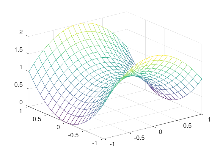
Figure 29.4: Demonstration of the use of interpn