15.2.1 Two-Dimensional Plots 
The plot function allows you to create simple x-y plots with
linear axes. For example,
x = -10:0.1:10;
plot (x, sin (x));
xlabel ("x");
ylabel ("sin (x)");
title ("Simple 2-D Plot");
displays a sine wave shown in Figure 15.1. On most systems, this command will open a separate plot window to display the graph.
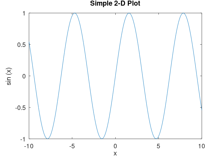
Figure 15.1: Simple Two-Dimensional Plot.
- : plot
(y)¶ - : plot
(x, y)¶ - : plot
(x, y, fmt)¶ - : plot
(…, property, value, …)¶ - : plot
(x1, y1, …, xn, yn)¶ - : plot
(hax, …)¶ - :
h =plot(…)¶ Produce 2-D plots.
Many different combinations of arguments are possible. The simplest form is
plot (y)
where the argument is taken as the set of y coordinates and the x coordinates are taken to be the range
1:numel (y).If more than one argument is given, they are interpreted as
plot (y, property, value, ...)
or
plot (x, y, property, value, ...)
or
plot (x, y, fmt, ...)
and so on. Any number of argument sets may appear. The x and y values are interpreted as follows:
- If a single data argument is supplied, it is taken as the set of y coordinates and the x coordinates are taken to be the indices of the elements, starting with 1.
- If x and y are scalars, a single point is plotted.
squeeze()is applied to arguments with more than two dimensions, but no more than two singleton dimensions.- If either x or y is a scalar and the other is a vector, a series of points are plotted at the coordinates defined by the scalar and each element of the vector.
- If both arguments are vectors, the elements of y are plotted versus the elements of x.
- If x is a vector and y is a matrix, then the columns (or rows) of y are plotted versus x. (using whichever combination matches, with columns tried first.)
- If the x is a matrix and y is a vector, y is plotted versus the columns (or rows) of x. (using whichever combination matches, with columns tried first.)
- If both arguments are matrices, the columns of y are plotted versus the columns of x. In this case, both matrices must have the same number of rows and columns and no attempt is made to transpose the arguments to make the number of rows match.
Multiple property-value pairs may be specified, but they must appear in pairs. These arguments are applied to the line objects drawn by
plot. Useful properties to modify are"linestyle","linewidth","color","marker","markersize","markeredgecolor","markerfacecolor". The full list of properties is documented at Line Properties.The fmt format argument can also be used to control the plot style. It is a string composed of four optional parts: "<linestyle><marker><color><;displayname;>". When a marker is specified, but no linestyle, only the markers are plotted. Similarly, if a linestyle is specified, but no marker, then only lines are drawn. If both are specified then lines and markers will be plotted. If no fmt and no property/value pairs are given, then the default plot style is solid lines with no markers and the color determined by the
"colororder"property of the current axes.Format arguments:
- linestyle
-
‘-’ Use solid lines (default). ‘--’ Use dashed lines. ‘:’ Use dotted lines. ‘-.’ Use dash-dotted lines. - marker
-
‘+’ crosshair ‘o’ circle ‘*’ star ‘.’ point ‘x’ cross ‘|’ vertical line ‘_’ horizontal line ‘s’ square ‘d’ diamond ‘^’ upward-facing triangle ‘v’ downward-facing triangle ‘>’ right-facing triangle ‘<’ left-facing triangle ‘p’ pentagram ‘h’ hexagram - color
-
‘k’, "black"blacK ‘r’, "red"Red ‘g’, "green"Green ‘b’, "blue"Blue ‘y’, "yellow"Yellow ‘m’, "magenta"Magenta ‘c’, "cyan"Cyan ‘w’, "white"White ";displayname;"The text between semicolons is used to set the
"displayname"property which determines the label used for the plot legend.
The fmt argument may also be used to assign legend labels. To do so, include the desired label between semicolons after the formatting sequence described above, e.g.,
"+b;Data Series 3;". Note that the last semicolon is required and Octave will generate an error if it is left out.Here are some plot examples:
plot (x, y, "or", x, y2, x, y3, "m", x, y4, "+")
This command will plot
ywith red circles,y2with solid lines,y3with solid magenta lines, andy4with points displayed as ‘+’.plot (b, "*", "markersize", 10)
This command will plot the data in the variable
b, with points displayed as ‘*’ and a marker size of 10.t = 0:0.1:6.3; plot (t, cos(t), "-;cos(t);", t, sin(t), "-b;sin(t);");
This will plot the cosine and sine functions and label them accordingly in the legend.
If the first argument hax is an axes handle, then plot into this axes, rather than the current axes returned by
gca.The optional return value h is a vector of graphics handles to the created line objects.
To save a plot, in one of several image formats such as PostScript or PNG, use the
printcommand.See also: axis, box, grid, hold, legend, title, xlabel, ylabel, xlim, ylim, ezplot, errorbar, fplot, line, plot3, polar, loglog, semilogx, semilogy, subplot.
The plotyy function may be used to create a plot with two
independent y axes.
- : plotyy
(x1, y1, x2, y2)¶ - : plotyy
(…, fcn)¶ - : plotyy
(…, fun1, fun2)¶ - : plotyy
(hax, …)¶ - :
[ax, h1, h2] =plotyy(…)¶ Plot two sets of data with independent y-axes and a common x-axis.
The arguments x1 and y1 define the arguments for the first plot and x1 and y2 for the second.
By default the arguments are evaluated with
feval (@plot, x, y). However the type of plot can be modified with the fcn argument, in which case the plots are generated byfeval (fcn, x, y). fcn can be a function handle, an inline function, or a string of a function name.The function to use for each of the plots can be independently defined with fun1 and fun2.
The first argument hax can be an axes handle to the principal axes in which to plot the x1 and y1 data. It can also be a two-element vector with the axes handles to the primary and secondary axes (see output ax).
The return value ax is a vector with the axes handles of the two y-axes. h1 and h2 are handles to the objects generated by the plot commands.
x = 0:0.1:2*pi;
y1 = sin (x);
y2 = exp (x - 1);
ax = plotyy (x, y1, x - 1, y2, @plot, @semilogy);
xlabel ("X");
ylabel (ax(1), "Axis 1");
ylabel (ax(2), "Axis 2");
When using
plotyyin conjunction withsubplotmake sure to callsubplotfirst and pass the resulting axes handle toplotyy. Do not callsubplotwith any of the axes handles returned byplotyyor the other axes will be removed.
The functions semilogx, semilogy, and loglog are
similar to the plot function, but produce plots in which one or
both of the axes use log scales.
- : semilogx
(y)¶ - : semilogx
(x, y)¶ - : semilogx
(x, y, property, value, …)¶ - : semilogx
(x, y, fmt)¶ - : semilogx
(hax, …)¶ - :
h =semilogx(…)¶ Produce a 2-D plot using a logarithmic scale for the x-axis.
See the documentation of
plotfor a description of the arguments thatsemilogxwill accept.If the first argument hax is an axes handle, then plot into this axes, rather than the current axes returned by
gca.The optional return value h is a graphics handle to the created plot.
- : semilogy
(y)¶ - : semilogy
(x, y)¶ - : semilogy
(x, y, property, value, …)¶ - : semilogy
(x, y, fmt)¶ - : semilogy
(h, …)¶ - :
h =semilogy(…)¶ Produce a 2-D plot using a logarithmic scale for the y-axis.
See the documentation of
plotfor a description of the arguments thatsemilogywill accept.If the first argument hax is an axes handle, then plot into this axes, rather than the current axes returned by
gca.The optional return value h is a graphics handle to the created plot.
- : loglog
(y)¶ - : loglog
(x, y)¶ - : loglog
(x, y, prop, value, …)¶ - : loglog
(x, y, fmt)¶ - : loglog
(hax, …)¶ - :
h =loglog(…)¶ Produce a 2-D plot using logarithmic scales for both axes.
See the documentation of
plotfor a description of the arguments thatloglogwill accept.If the first argument hax is an axes handle, then plot into this axes, rather than the current axes returned by
gca.The optional return value h is a graphics handle to the created plot.
The functions bar, barh, stairs, and stem
are useful for displaying discrete data. For example,
randn ("state", 1);
hist (randn (10000, 1), 30);
xlabel ("Value");
ylabel ("Count");
title ("Histogram of 10,000 normally distributed random numbers");
produces the histogram of 10,000 normally distributed random numbers
shown in Figure 15.2. Note that, randn ("state", 1);, initializes
the random number generator for randn to a known value so that the
returned values are reproducible; This guarantees that the figure produced
is identical to the one in this manual.
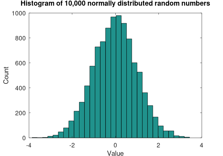
Figure 15.2: Histogram.
- : bar
(y)¶ - : bar
(x, y)¶ - : bar
(…, w)¶ - : bar
(…, style)¶ - : bar
(…, prop, val, …)¶ - : bar
(hax, …)¶ - :
h =bar(…, prop, val, …)¶ Produce a bar graph from two vectors of X-Y data.
If only one argument is given, y, it is taken as a vector of Y values and the X coordinates are the range
1:numel (y).The optional input w controls the width of the bars. A value of 1.0 will cause each bar to exactly touch any adjacent bars. The default width is 0.8.
If y is a matrix, then each column of y is taken to be a separate bar graph plotted on the same graph. By default the columns are plotted side-by-side. This behavior can be changed by the style argument which can take the following values:
"grouped"(default)Side-by-side bars with a gap between bars and centered over the X-coordinate.
"stacked"Bars are stacked so that each X value has a single bar composed of multiple segments.
"hist"Side-by-side bars with no gap between bars and centered over the X-coordinate.
"histc"Side-by-side bars with no gap between bars and left-aligned to the X-coordinate.
Optional property/value pairs are passed directly to the underlying patch objects. The full list of properties is documented at Patch Properties.
If the first argument hax is an axes handle, then plot into this axes, rather than the current axes returned by
gca.The optional return value h is a vector of handles to the created "bar series" hggroups with one handle per column of the variable y. This series makes it possible to change a common element in one bar series object and have the change reflected in the other "bar series". For example,
h = bar (rand (5, 10));
set (h(1), "basevalue", 0.5);
changes the position on the base of all of the bar series.
The following example modifies the face and edge colors using property/value pairs.
bar (randn (1, 100), "facecolor", "r", "edgecolor", "b");
The default color for bars is taken from the axes’
"ColorOrder"property. The default color for bars when a histogram option ("hist","histc"is used is the"Colormap"property of either the axes or figure. The color of bars can also be set manually using the"facecolor"property as shown below.h = bar (rand (10, 3)); set (h(1), "facecolor", "r") set (h(2), "facecolor", "g") set (h(3), "facecolor", "b")
- : barh
(y)¶ - : barh
(x, y)¶ - : barh
(…, w)¶ - : barh
(…, style)¶ - : barh
(…, prop, val, …)¶ - : barh
(hax, …)¶ - :
h =barh(…, prop, val, …)¶ Produce a horizontal bar graph from two vectors of X-Y data.
If only one argument is given, it is taken as a vector of Y values and the X coordinates are the range
1:numel (y).The optional input w controls the width of the bars. A value of 1.0 will cause each bar to exactly touch any adjacent bars. The default width is 0.8.
If y is a matrix, then each column of y is taken to be a separate bar graph plotted on the same graph. By default the columns are plotted side-by-side. This behavior can be changed by the style argument which can take the following values:
"grouped"(default)Side-by-side bars with a gap between bars and centered over the Y-coordinate.
"stacked"Bars are stacked so that each Y value has a single bar composed of multiple segments.
"hist"Side-by-side bars with no gap between bars and centered over the Y-coordinate.
"histc"Side-by-side bars with no gap between bars and left-aligned to the Y-coordinate.
Optional property/value pairs are passed directly to the underlying patch objects. The full list of properties is documented at Patch Properties.
If the first argument hax is an axes handle, then plot into this axes, rather than the current axes returned by
gca.The optional return value h is a graphics handle to the created bar series hggroup. For a description of the use of the bar series, see
bar.
- : hist
(y)¶ - : hist
(y, nbins)¶ - : hist
(y, x)¶ - : hist
(y, x, norm)¶ - : hist
(…, prop, val, …)¶ - : hist
(hax, …)¶ - :
[nn, xx] =hist(…)¶ Produce histogram counts or plots.
With one vector input argument, y, plot a histogram of the values with 10 bins. The range of the histogram bins is determined by the range of the data (difference between maximum and minimum value in y). Extreme values are lumped into the first and last bins. If y is a matrix then plot a histogram where each bin contains one bar per input column of y.
If the optional second argument is a scalar, nbins, it defines the number of bins.
If the optional second argument is a vector, x, it defines the centers of the bins. The width of the bins is determined from the adjacent values in the vector. The total number of bins is
numel (x).If a third argument norm is provided, the histogram is normalized. In case norm is a positive scalar, the resulting bars are normalized to norm. If norm is a vector of positive scalars of length
columns (y), then the resulting bar ofy(:,i)is normalized tonorm(i).[nn, xx] = hist (rand (10, 3), 5, [1 2 3]); sum (nn, 1) ⇒ ans = 1 2 3The histogram’s appearance may be modified by specifying property/value pairs to the underlying patch object. For example, the face and edge color may be modified:
hist (randn (1, 100), 25, "facecolor", "r", "edgecolor", "b");
The full list of patch properties is documented at Patch Properties. property. If not specified, the default colors for the histogram are taken from the
"Colormap"property of the axes or figure.If the first argument hax is an axes handle, then plot into this axes, rather than the current axes returned by
gca.If an output is requested then no plot is made. Instead, return the values nn (numbers of elements) and xx (bin centers) such that
bar (xx, nn)will plot the histogram.
- : stemleaf
(x, caption)¶ - : stemleaf
(x, caption, stem_sz)¶ - :
plotstr =stemleaf(…)¶ Compute and display a stem and leaf plot of the vector x.
The input x should be a vector of integers. Any non-integer values will be converted to integer by
x = fix (x). By default each element of x will be plotted with the last digit of the element as a leaf value and the remaining digits as the stem. For example, 123 will be plotted with the stem ‘12’ and the leaf ‘3’. The second argument, caption, should be a character array which provides a description of the data. It is included as a heading for the output.The optional input stem_sz sets the width of each stem. The stem width is determined by
10^(stem_sz + 1). The default stem width is 10.The output of
stemleafis composed of two parts: a "Fenced Letter Display", followed by the stem-and-leaf plot itself. The Fenced Letter Display is described in Exploratory Data Analysis. Briefly, the entries are as shown:Fenced Letter Display #% nx|___________________ nx = numel (x) M% mi| md | mi median index, md median H% hi|hl hu| hs hi lower hinge index, hl,hu hinges, 1 |x(1) x(nx)| hs h_spreadx(1), x(nx) first _______ and last data value. ______|step |_______ step 1.5*h_spread f|ifl ifh| inner fence, lower and higher |nfl nfh| no.\ of data points within fences F|ofl ofh| outer fence, lower and higher |nFl nFh| no.\ of data points outside outer fencesThe stem-and-leaf plot shows on each line the stem value followed by the string made up of the leaf digits. If the stem_sz is not 1 the successive leaf values are separated by ",".
With no return argument, the plot is immediately displayed. If an output argument is provided, the plot is returned as an array of strings.
The leaf digits are not sorted. If sorted leaf values are desired, use
xs = sort (x)before callingstemleaf (xs).The stem and leaf plot and associated displays are described in: Chapter 3, Exploratory Data Analysis by J. W. Tukey, Addison-Wesley, 1977.
- : printd
(obj, filename)¶ - :
out_file =printd(…)¶ -
Convert any object acceptable to
dispinto the format selected by the suffix of filename.If the optional output out_file is requested, the name of the created file is returned.
This function is intended to facilitate manipulation of the output of functions such as
stemleaf.See also: stemleaf.
- : stairs
(y)¶ - : stairs
(x, y)¶ - : stairs
(…, style)¶ - : stairs
(…, prop, val, …)¶ - : stairs
(hax, …)¶ - :
h =stairs(…)¶ - :
[xstep, ystep] =stairs(…)¶ Produce a stairstep plot.
The arguments x and y may be vectors or matrices. If only one argument is given, it is taken as a vector of Y values and the X coordinates are taken to be the indices of the elements (
x = 1:numel (y)).The style to use for the plot can be defined with a line style style of the same format as the
plotcommand.Multiple property/value pairs may be specified, but they must appear in pairs. The full list of properties is documented at Line Properties.
If the first argument hax is an axes handle, then plot into this axes, rather than the current axes returned by
gca.If one output argument is requested, return a graphics handle to the created plot. If two output arguments are specified, the data are generated but not plotted. For example,
stairs (x, y);
and
[xs, ys] = stairs (x, y);
plot (xs, ys);
are equivalent.
- : stem
(y)¶ - : stem
(x, y)¶ - : stem
(…, linespec)¶ - : stem
(…, "filled")¶ - : stem
(…, prop, val, …)¶ - : stem
(hax, …)¶ - :
h =stem(…)¶ Plot a 2-D stem graph.
If only one argument is given, it is taken as the y-values and the x-coordinates are taken from the indices of the elements.
If y is a matrix, then each column of the matrix is plotted as a separate stem graph. In this case x can either be a vector, the same length as the number of rows in y, or it can be a matrix of the same size as y.
The default color is
"b"(blue), the default line style is"-", and the default marker is"o". The line style can be altered by the linespec argument in the same manner as theplotcommand. If the"filled"argument is present the markers at the top of the stems will be filled in. For example,x = 1:10; y = 2*x; stem (x, y, "r");
plots 10 stems with heights from 2 to 20 in red;
Optional property/value pairs may be specified to control the appearance of the plot. The full list of properties is documented at Line Properties.
If the first argument hax is an axes handle, then plot into this axes, rather than the current axes returned by
gca.The optional return value h is a handle to a "stem series" hggroup. The single hggroup handle has all of the graphical elements comprising the plot as its children; This allows the properties of multiple graphics objects to be changed by modifying just a single property of the "stem series" hggroup.
For example,
x = [0:10]';
y = [sin(x), cos(x)]
h = stem (x, y);
set (h(2), "color", "g");
set (h(1), "basevalue", -1)
changes the color of the second "stem series" and moves the base line of the first.
Stem Series Properties
- linestyle
The linestyle of the stem. (Default:
"-")- linewidth
The width of the stem. (Default: 0.5)
- color
The color of the stem, and if not separately specified, the marker. (Default:
"b"[blue])- marker
The marker symbol to use at the top of each stem. (Default:
"o")- markeredgecolor
The edge color of the marker. (Default:
"color"property)- markerfacecolor
The color to use for "filling" the marker. (Default:
"none"[unfilled])- markersize
The size of the marker. (Default: 6)
- baseline
The handle of the line object which implements the baseline. Use
setwith the returned handle to change graphic properties of the baseline.- basevalue
The y-value where the baseline is drawn. (Default: 0)
- : stem3
(x, y, z)¶ - : stem3
(…, linespec)¶ - : stem3
(…, "filled")¶ - : stem3
(…, prop, val, …)¶ - : stem3
(hax, …)¶ - :
h =stem3(…)¶ Plot a 3-D stem graph.
Stems are drawn from the height z to the location in the x-y plane determined by x and y. The default color is
"b"(blue), the default line style is"-", and the default marker is"o".The line style can be altered by the linespec argument in the same manner as the
plotcommand. If the"filled"argument is present the markers at the top of the stems will be filled in.Optional property/value pairs may be specified to control the appearance of the plot. The full list of properties is documented at Line Properties.
If the first argument hax is an axes handle, then plot into this axes, rather than the current axes returned by
gca.The optional return value h is a handle to the "stem series" hggroup containing the line and marker objects used for the plot. See
stem, for a description of the "stem series" object.Example:
theta = 0:0.2:6;
stem3 (cos (theta), sin (theta), theta);
plots 31 stems with heights from 0 to 6 lying on a circle.
Implementation Note: Color definitions with RGB-triples are not valid.
- : scatter
(x, y)¶ - : scatter
(x, y, s)¶ - : scatter
(x, y, s, c)¶ - : scatter
(…, style)¶ - : scatter
(…, "filled")¶ - : scatter
(…, prop, val, …)¶ - : scatter
(hax, …)¶ - :
h =scatter(…)¶ Draw a 2-D scatter plot.
A marker is plotted at each point defined by the coordinates in the vectors x and y.
The size of the markers is determined by s, which can be a scalar or a vector of the same length as x and y. If s is not given, or is an empty matrix, then a default value of 36 square points is used (The marker size itself is
sqrt (s)).The color of the markers is determined by c, which can be a string defining a fixed color; a 3-element vector giving the red, green, and blue components of the color; a vector of the same length as x that gives a scaled index into the current colormap; or an Nx3 matrix defining the RGB color of each marker individually.
The marker to use can be changed with the style argument; it is a string defining a marker in the same manner as the
plotcommand. If no marker is specified it defaults to"o"or circles. If the argument"filled"is given then the markers are filled.If the first argument hax is an axes handle, then plot into this axes, rather than the current axes returned by
gca.The optional return value h is a graphics handle to the created scatter object.
Example:
x = randn (100, 1);
y = randn (100, 1);
scatter (x, y, [], sqrt (x.^2 + y.^2));
Programming Note: The full list of properties is documented at Scatter Properties.
- : plotmatrix
(x, y)¶ - : plotmatrix
(x)¶ - : plotmatrix
(…, style)¶ - : plotmatrix
(hax, …)¶ - :
[h, ax, bigax, p, pax] =plotmatrix(…)¶ Scatter plot of the columns of one matrix against another.
Given the arguments x and y that have a matching number of rows,
plotmatrixplots a set of axes corresponding toplot (x(:, i), y(:, j))
When called with a single argument x this is equivalent to
plotmatrix (x, x)
except that the diagonal of the set of axes will be replaced with the histogram
hist (x(:, i)).The marker to use can be changed with the style argument, that is a string defining a marker in the same manner as the
plotcommand.If the first argument hax is an axes handle, then plot into this axes, rather than the current axes returned by
gca.The optional return value h provides handles to the individual graphics objects in the scatter plots, whereas ax returns the handles to the scatter plot axes objects.
bigax is a hidden axes object that surrounds the other axes, such that the commands
xlabel,title, etc., will be associated with this hidden axes.Finally, p returns the graphics objects associated with the histogram and pax the corresponding axes objects.
Example:
plotmatrix (randn (100, 3), "g+")
- : pareto
(y)¶ - : pareto
(y, x)¶ - : pareto
(hax, …)¶ - :
h =pareto(…)¶ Draw a Pareto chart.
A Pareto chart is a bar graph that arranges information in such a way that priorities for process improvement can be established; It organizes and displays information to show the relative importance of data. The chart is similar to the histogram or bar chart, except that the bars are arranged in decreasing magnitude from left to right along the x-axis.
The fundamental idea (Pareto principle) behind the use of Pareto diagrams is that the majority of an effect is due to a small subset of the causes. For quality improvement, the first few contributing causes (leftmost bars as presented on the diagram) to a problem usually account for the majority of the result. Thus, targeting these "major causes" for elimination results in the most cost-effective improvement scheme.
Typically only the magnitude data y is present in which case x is taken to be the range
1 : length (y). If x is given it may be a string array, a cell array of strings, or a numerical vector.If the first argument hax is an axes handle, then plot into this axes, rather than the current axes returned by
gca.The optional return value h is a 2-element vector with a graphics handle for the created bar plot and a second handle for the created line plot.
An example of the use of
paretoisCheese = {"Cheddar", "Swiss", "Camembert", ... "Munster", "Stilton", "Blue"}; Sold = [105, 30, 70, 10, 15, 20]; pareto (Sold, Cheese);
- : rose
(theta)¶ - : rose
(theta, nbins)¶ - : rose
(theta, bins)¶ - : rose
(hax, …)¶ - :
h =rose(…)¶ - :
[th r] =rose(…)¶ Plot an angular histogram.
With one vector argument, th, plot the histogram with 20 angular bins. If th is a matrix then each column of th produces a separate histogram.
If nbins is given and is a scalar, then the histogram is produced with nbin bins. If bins is a vector, then the center of each bin is defined by the values in bins and the number of bins is given by the number of elements in bins.
If the first argument hax is an axes handle, then plot into this axes, rather than the current axes returned by
gca.The optional return value h is a vector of graphics handles to the line objects representing each histogram.
If two output arguments are requested then no plot is made and the polar vectors necessary to plot the histogram are returned instead.
Example
[th, r] = rose ([2*randn(1e5,1), pi + 2*randn(1e5,1)]);
polar (th, r);
The contour, contourf and contourc functions
produce two-dimensional contour plots from three-dimensional data.
- : contour
(z)¶ - : contour
(z, vn)¶ - : contour
(x, y, z)¶ - : contour
(x, y, z, vn)¶ - : contour
(…, style)¶ - : contour
(hax, …)¶ - :
[c, h] =contour(…)¶ Create a 2-D contour plot.
Plot level curves (contour lines) of the matrix z, using the contour matrix c computed by
contourcfrom the same arguments; see the latter for their interpretation.The appearance of contour lines can be defined with a line style style in the same manner as
plot. Only line style and color are used; Any markers defined by style are ignored.If the first argument hax is an axes handle, then plot into this axes, rather than the current axes returned by
gca.The optional output c contains the contour levels in
contourcformat.The optional return value h is a graphics handle to the hggroup comprising the contour lines.
Example:
x = 0:3;
y = 0:2;
z = y' * x;
contour (x, y, z, 2:3)
See also: ezcontour, contourc, contourf, contour3, clabel, meshc, surfc, caxis, colormap, plot.
- : contourf
(z)¶ - : contourf
(z, vn)¶ - : contourf
(x, y, z)¶ - : contourf
(x, y, z, vn)¶ - : contourf
(…, style)¶ - : contourf
(hax, …)¶ - :
[c, h] =contourf(…)¶ Create a 2-D contour plot with filled intervals.
Plot level curves (contour lines) of the matrix z and fill the region between lines with colors from the current colormap.
The level curves are taken from the contour matrix c computed by
contourcfor the same arguments; see the latter for their interpretation.The appearance of contour lines can be defined with a line style style in the same manner as
plot. Only line style and color are used; Any markers defined by style are ignored.If the first argument hax is an axes handle, then plot into this axes, rather than the current axes returned by
gca.The optional output c contains the contour levels in
contourcformat.The optional return value h is a graphics handle to the hggroup comprising the contour lines.
The following example plots filled contours of the
peaksfunction.[x, y, z] = peaks (50); contourf (x, y, z, -7:9)
See also: ezcontourf, contour, contourc, contour3, clabel, meshc, surfc, caxis, colormap, plot.
- :
c =contourc(z)¶ - :
c =contourc(z, vn)¶ - :
c =contourc(x, y, z)¶ - :
c =contourc(x, y, z, vn)¶ - :
[c, lev] =contourc(…)¶ Compute contour lines (isolines of constant Z value).
The matrix z contains height values above the rectangular grid determined by x and y. If only a single input z is provided then x is taken to be
1:columns (z)and y is taken to be1:rows (z). The minimum data size is 2x2.The optional input vn is either a scalar denoting the number of contour lines to compute or a vector containing the Z values where lines will be computed. When vn is a vector the number of contour lines is
numel (vn). However, to compute a single contour line at a given value usevn = [val, val]. If vn is omitted it defaults to 10.The return value c is a 2xn matrix containing the contour lines in the following format
c = [lev1, x1, x2, ..., levn, x1, x2, ...
     len1, y1, y2, ..., lenn, y1, y2, ...]
in which contour line n has a level (height) of levn and length of lenn.
The optional return value lev is a vector with the Z values of the contour levels.
Example:
x = 0:2;
y = x;
z = x' * y;
c = contourc (x, y, z, 2:3)
  ⇒ c =
        2.0000   1.0000   1.0000   2.0000   2.0000   3.0000   1.5000   2.0000
        4.0000   2.0000   2.0000   1.0000   1.0000   2.0000   2.0000   1.5000
- : contour3
(z)¶ - : contour3
(z, vn)¶ - : contour3
(x, y, z)¶ - : contour3
(x, y, z, vn)¶ - : contour3
(…, style)¶ - : contour3
(hax, …)¶ - :
[c, h] =contour3(…)¶ Create a 3-D contour plot.
contour3plots level curves (contour lines) of the matrix z at a Z level corresponding to each contour. This is in contrast tocontourwhich plots all of the contour lines at the same Z level and produces a 2-D plot.The level curves are taken from the contour matrix c computed by
contourcfor the same arguments; see the latter for their interpretation.The appearance of contour lines can be defined with a line style style in the same manner as
plot. Only line style and color are used; Any markers defined by style are ignored.If the first argument hax is an axes handle, then plot into this axes, rather than the current axes returned by
gca.The optional output c are the contour levels in
contourcformat.The optional return value h is a graphics handle to the hggroup comprising the contour lines.
Example:
contour3 (peaks (19));
colormap cool;
hold on;
surf (peaks (19), "facecolor", "none", "edgecolor", "black");
See also: contour, contourc, contourf, clabel, meshc, surfc, caxis, colormap, plot.
The errorbar, semilogxerr, semilogyerr, and
loglogerr functions produce plots with error bar markers. For
example,
rand ("state", 2);
x = 0:0.1:10;
y = sin (x);
lerr = 0.1 .* rand (size (x));
uerr = 0.1 .* rand (size (x));
errorbar (x, y, lerr, uerr);
axis ([0, 10, -1.1, 1.1]);
xlabel ("x");
ylabel ("sin (x)");
title ("Errorbar plot of sin (x)");
produces the figure shown in Figure 15.3.
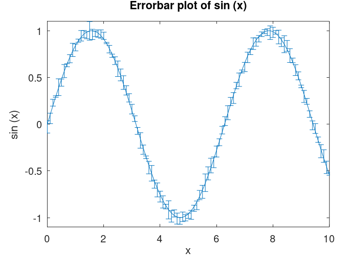
Figure 15.3: Errorbar plot.
- : errorbar
(y, ey)¶ - : errorbar
(y, …, fmt)¶ - : errorbar
(x, y, ey)¶ - : errorbar
(x, y, err, fmt)¶ - : errorbar
(x, y, lerr, uerr, fmt)¶ - : errorbar
(x, y, ex, ey, fmt)¶ - : errorbar
(x, y, lx, ux, ly, uy, fmt)¶ - : errorbar
(x1, y1, …, fmt, xn, yn, …)¶ - : errorbar
(hax, …)¶ - :
h =errorbar(…)¶ Create a 2-D plot with errorbars.
Many different combinations of arguments are possible. The simplest form is
errorbar (y, ey)
where the first argument is taken as the set of y coordinates, the second argument ey are the errors around the y values, and the x coordinates are taken to be the indices of the elements (
1:numel (y)).The general form of the function is
errorbar (x, y, err1, ..., fmt, ...)
After the x and y arguments there can be 1, 2, or 4 parameters specifying the error values depending on the nature of the error values and the plot format fmt.
- err (scalar)
When the error is a scalar all points share the same error value. The errorbars are symmetric and are drawn from data-err to data+err. The fmt argument determines whether err is in the x-direction, y-direction (default), or both.
- err (vector or matrix)
Each data point has a particular error value. The errorbars are symmetric and are drawn from data(n)-err(n) to data(n)+err(n).
- lerr, uerr (scalar)
The errors have a single low-side value and a single upper-side value. The errorbars are not symmetric and are drawn from data-lerr to data+uerr.
- lerr, uerr (vector or matrix)
Each data point has a low-side error and an upper-side error. The errorbars are not symmetric and are drawn from data(n)-lerr(n) to data(n)+uerr(n).
Any number of data sets (x1,y1, x2,y2, …) may appear as long as they are separated by a format string fmt.
If y is a matrix, x and the error parameters must also be matrices having the same dimensions. The columns of y are plotted versus the corresponding columns of x and errorbars are taken from the corresponding columns of the error parameters.
If fmt is missing, the yerrorbars ("~") plot style is assumed.
If the fmt argument is supplied then it is interpreted, as in normal plots, to specify the line style, marker, and color. In addition, fmt may include an errorbar style which must precede the ordinary format codes. The following errorbar styles are supported:
- ‘~’
Set yerrorbars plot style (default).
- ‘>’
Set xerrorbars plot style.
- ‘~>’
Set xyerrorbars plot style.
- ‘#~’
Set yboxes plot style.
- ‘#’
Set xboxes plot style.
- ‘#~>’
Set xyboxes plot style.
If the first argument hax is an axes handle, then plot into this axes, rather than the current axes returned by
gca.The optional return value h is a handle to the hggroup object representing the data plot and errorbars.
Note: For compatibility with MATLAB a line is drawn through all data points. However, most scientific errorbar plots are a scatter plot of points with errorbars. To accomplish this, add a marker style to the fmt argument such as
".". Alternatively, remove the line by modifying the returned graphic handle withset (h, "linestyle", "none").Examples:
errorbar (x, y, ex, ">.r")
produces an xerrorbar plot of y versus x with x errorbars drawn from x-ex to x+ex. The marker
"."is used so no connecting line is drawn and the errorbars appear in red.errorbar (x, y1, ey, "~", x, y2, ly, uy)produces yerrorbar plots with y1 and y2 versus x. Errorbars for y1 are drawn from y1-ey to y1+ey, errorbars for y2 from y2-ly to y2+uy.
errorbar (x, y, lx, ux,
          ly, uy, "~>")
produces an xyerrorbar plot of y versus x in which x errorbars are drawn from x-lx to x+ux and y errorbars from y-ly to y+uy.
See also: semilogxerr, semilogyerr, loglogerr, plot.
- : semilogxerr
(y, ey)¶ - : semilogxerr
(y, …, fmt)¶ - : semilogxerr
(x, y, ey)¶ - : semilogxerr
(x, y, err, fmt)¶ - : semilogxerr
(x, y, lerr, uerr, fmt)¶ - : semilogxerr
(x, y, ex, ey, fmt)¶ - : semilogxerr
(x, y, lx, ux, ly, uy, fmt)¶ - : semilogxerr
(x1, y1, …, fmt, xn, yn, …)¶ - : semilogxerr
(hax, …)¶ - :
h =semilogxerr(…)¶ Produce 2-D plots using a logarithmic scale for the x-axis and errorbars at each data point.
Many different combinations of arguments are possible. The most common form is
semilogxerr (x, y, ey, fmt)
which produces a semi-logarithmic plot of y versus x with errors in the y-scale defined by ey and the plot format defined by fmt. See
errorbar, for available formats and additional information.If the first argument hax is an axes handle, then plot into this axes, rather than the current axes returned by
gca.See also: errorbar, semilogyerr, loglogerr.
- : semilogyerr
(y, ey)¶ - : semilogyerr
(y, …, fmt)¶ - : semilogyerr
(x, y, ey)¶ - : semilogyerr
(x, y, err, fmt)¶ - : semilogyerr
(x, y, lerr, uerr, fmt)¶ - : semilogyerr
(x, y, ex, ey, fmt)¶ - : semilogyerr
(x, y, lx, ux, ly, uy, fmt)¶ - : semilogyerr
(x1, y1, …, fmt, xn, yn, …)¶ - : semilogyerr
(hax, …)¶ - :
h =semilogyerr(…)¶ Produce 2-D plots using a logarithmic scale for the y-axis and errorbars at each data point.
Many different combinations of arguments are possible. The most common form is
semilogyerr (x, y, ey, fmt)
which produces a semi-logarithmic plot of y versus x with errors in the y-scale defined by ey and the plot format defined by fmt. See
errorbar, for available formats and additional information.If the first argument hax is an axes handle, then plot into this axes, rather than the current axes returned by
gca.See also: errorbar, semilogxerr, loglogerr.
- : loglogerr
(y, ey)¶ - : loglogerr
(y, …, fmt)¶ - : loglogerr
(x, y, ey)¶ - : loglogerr
(x, y, err, fmt)¶ - : loglogerr
(x, y, lerr, uerr, fmt)¶ - : loglogerr
(x, y, ex, ey, fmt)¶ - : loglogerr
(x, y, lx, ux, ly, uy, fmt)¶ - : loglogerr
(x1, y1, …, fmt, xn, yn, …)¶ - : loglogerr
(hax, …)¶ - :
h =loglogerr(…)¶ Produce 2-D plots on a double logarithm axis with errorbars.
Many different combinations of arguments are possible. The most common form is
loglogerr (x, y, ey, fmt)
which produces a double logarithm plot of y versus x with errors in the y-scale defined by ey and the plot format defined by fmt. See
errorbar, for available formats and additional information.If the first argument hax is an axes handle, then plot into this axes, rather than the current axes returned by
gca.See also: errorbar, semilogxerr, semilogyerr.
Finally, the polar function allows you to easily plot data in
polar coordinates. However, the display coordinates remain rectangular
and linear. For example,
polar (0:0.1:10*pi, 0:0.1:10*pi);
title ("Example polar plot from 0 to 10*pi");
produces the spiral plot shown in Figure 15.4.
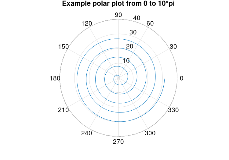
Figure 15.4: Polar plot.
- : polar
(theta, rho)¶ - : polar
(theta, rho, fmt)¶ - : polar
(cplx)¶ - : polar
(cplx, fmt)¶ - : polar
(hax, …)¶ - :
h =polar(…)¶ Create a 2-D plot from polar coordinates theta and rho.
The input theta is assumed to be radians and is converted to degrees for plotting. If you have degrees then you must convert (see
cart2pol) to radians before passing the data to this function.If a single complex input cplx is given then the real part is used for theta and the imaginary part is used for rho.
The optional argument fmt specifies the line format in the same way as
plot.If the first argument hax is an axes handle, then plot into this axes, rather than the current axes returned by
gca.The optional return value h is a graphics handle to the created plot.
Implementation Note: The polar axis is drawn using line and text objects encapsulated in an hggroup. The hggroup properties are linked to the original axes object such that altering an appearance property, for example
fontname, will update the polar axis. Two new properties are added to the original axes–rtick,ttick–which replacextick,ytick. The first is a list of tick locations in the radial (rho) direction; The second is a list of tick locations in the angular (theta) direction specified in degrees, i.e., in the range 0–359.
- : pie
(x)¶ - : pie
(…, explode)¶ - : pie
(…, labels)¶ - : pie
(hax, …)¶ - :
h =pie(…)¶ Plot a 2-D pie chart.
When called with a single vector argument, produce a pie chart of the elements in x. The size of the ith slice is the percentage that the element xi represents of the total sum of x:
pct = x(i) / sum (x).The optional input explode is a vector of the same length as x that, if nonzero, "explodes" the slice from the pie chart.
The optional input labels is a cell array of strings of the same length as x specifying the label for each slice.
If the first argument hax is an axes handle, then plot into this axes, rather than the current axes returned by
gca.The optional return value h is a list of handles to the patch and text objects generating the plot.
Note: If
sum (x) ≤ 1then the elements of x are interpreted as percentages directly and are not normalized bysum (x). Furthermore, if the sum is less than 1 then there will be a missing slice in the pie plot to represent the missing, unspecified percentage.
- : pie3
(x)¶ - : pie3
(…, explode)¶ - : pie3
(…, labels)¶ - : pie3
(hax, …)¶ - :
h =pie3(…)¶ Plot a 3-D pie chart.
Called with a single vector argument, produces a 3-D pie chart of the elements in x. The size of the ith slice is the percentage that the element xi represents of the total sum of x:
pct = x(i) / sum (x).The optional input explode is a vector of the same length as x that, if nonzero, "explodes" the slice from the pie chart.
The optional input labels is a cell array of strings of the same length as x specifying the label for each slice.
If the first argument hax is an axes handle, then plot into this axes, rather than the current axes returned by
gca.The optional return value h is a list of graphics handles to the patch, surface, and text objects generating the plot.
Note: If
sum (x) ≤ 1then the elements of x are interpreted as percentages directly and are not normalized bysum (x). Furthermore, if the sum is less than 1 then there will be a missing slice in the pie plot to represent the missing, unspecified percentage.
- : quiver
(u, v)¶ - : quiver
(x, y, u, v)¶ - : quiver
(…, s)¶ - : quiver
(…, style)¶ - : quiver
(…, "filled")¶ - : quiver
(hax, …)¶ - :
h =quiver(…)¶ -
Plot a 2-D vector field with arrows.
Plot the (u, v) components of a vector field at the grid points defined by (x, y). If the grid is uniform then x and y can be specified as grid vectors and
meshgridis used to create the 2-D grid.If x and y are not given they are assumed to be
(1:m, 1:n)where[m, n] = size (u).The optional input s is a scalar defining a scaling factor to use for the arrows of the field relative to the mesh spacing. A value of 1.0 will result in the longest vector exactly filling one grid square. A value of 0 or
"off"disables all scaling. The default value is 0.9.The style to use for the plot can be defined with a line style, style, of the same format as the
plotcommand. If a marker is specified then the markers are drawn at the origin of the vectors (which are the grid points defined by x and y). When a marker is specified, the arrowhead is not drawn. If the argument"filled"is given then the markers are filled. If name-value plot style properties are used, they must appear in pairs and follow any other plot style arguments.If the first argument hax is an axes handle, then plot into this axes, rather than the current axes returned by
gca.The optional return value h is a graphics handle to a quiver object. A quiver object regroups the components of the quiver plot (body, arrow, and marker), and allows them to be changed together.
Example:
[x, y] = meshgrid (1:2:20);
h = quiver (x, y, sin (2*pi*x/10), sin (2*pi*y/10));
set (h, "maxheadsize", 0.33);
- : quiver3
(x, y, z, u, v, w)¶ - : quiver3
(z, u, v, w)¶ - : quiver3
(…, s)¶ - : quiver3
(…, style)¶ - : quiver3
(…, "filled")¶ - : quiver3
(hax, …)¶ - :
h =quiver3(…)¶ -
Plot a 3-D vector field with arrows.
Plot the (u, v, w) components of a vector field at the grid points defined by (x, y, z). If the grid is uniform then x, y, and z can be specified as grid vectors and
meshgridis used to create the 3-D grid.If x and y are not given they are assumed to be
(1:m, 1:n)where[m, n] = size (u).The optional input s is a scalar defining a scaling factor to use for the arrows of the field relative to the mesh spacing. A value of 1.0 will result in the longest vector exactly filling one grid cube. A value of 0 or
"off"disables all scaling. The default value is 0.9.The style to use for the plot can be defined with a line style style of the same format as the
plotcommand. If a marker is specified then the markers are drawn at the origin of the vectors (which are the grid points defined by x, y, z). When a marker is specified, the arrowhead is not drawn. If the argument"filled"is given then the markers are filled. If name-value plot style properties are used, they must appear in pairs and follow any other plot style arguments.If the first argument hax is an axes handle, then plot into this axes, rather than the current axes returned by
gca.The optional return value h is a graphics handle to a quiver object. A quiver object regroups the components of the quiver plot (body, arrow, and marker), and allows them to be changed together.
[x, y, z] = peaks (25);
surf (x, y, z);
hold on;
[u, v, w] = surfnorm (x, y, z / 10);
h = quiver3 (x, y, z, u, v, w);
set (h, "maxheadsize", 0.33);
- : streamribbon
(x, y, z, u, v, w, sx, sy, sz)¶ - : streamribbon
(u, v, w, sx, sy, sz)¶ - : streamribbon
(xyz, x, y, z, anlr_spd, lin_spd)¶ - : streamribbon
(xyz, anlr_spd, lin_spd)¶ - : streamribbon
(xyz, anlr_rot)¶ - : streamribbon
(…, width)¶ - : streamribbon
(hax, …)¶ - :
h =streamribbon(…)¶ Calculate and display streamribbons.
The streamribbon is constructed by rotating a normal vector around a streamline according to the angular rotation of the vector field.
The vector field is given by
[u, v, w]and is defined over a rectangular grid given by[x, y, z]. The streamribbons start at the seed points[sx, sy, sz].streamribboncan be called with a cell array that contains pre-computed streamline data. To do this, xyz must be created with thestream3function. lin_spd is the linear speed of the vector field and can be calculated from[u, v, w]by the square root of the sum of the squares. The angular speed anlr_spd is the projection of the angular velocity onto the velocity of the normalized vector field and can be calculated with thecurlcommand. This option is useful if you need to alter the integrator step size or the maximum number of streamline vertices.Alternatively, ribbons can be created from an array of vertices xyz of a path curve. anlr_rot contains the angles of rotation around the edges between adjacent vertices of the path curve.
The input parameter width sets the width of the streamribbons.
Streamribbons are colored according to the total angle of rotation along the ribbon.
If the first argument hax is an axes handle, then plot into this axes, rather than the current axes returned by
gca.The optional return value h is a graphics handle to the plot objects created for each streamribbon.
Example:
[x, y, z] = meshgrid (0:0.2:4, -1:0.2:1, -1:0.2:1);
u = - x + 10;
v = 10 * z.*x;
w = - 10 * y.*x;
streamribbon (x, y, z, u, v, w, [0, 0], [0, 0.6], [0, 0]);
view (3);
See also: streamline, stream3, streamtube, ostreamtube.
- : streamtube
(x, y, z, u, v, w, sx, sy, sz)¶ - : streamtube
(u, v, w, sx, sy, sz)¶ - : streamtube
(xyz, x, y, z, div)¶ - : streamtube
(xyz, div)¶ - : streamtube
(xyz, dia)¶ - : streamtube
(…, options)¶ - : streamtube
(hax, …)¶ - :
h =streamtube(…)¶ Plot tubes scaled by the divergence along streamlines.
streamtubedraws tubes whose diameter is scaled by the divergence of a vector field. The vector field is given by[u, v, w]and is defined over a rectangular grid given by[x, y, z]. The tubes start at the seed points[sx, sy, sz]and are plot along streamlines.streamtubecan also be called with a cell array containing pre-computed streamline data. To do this, xyz must be created with thestream3command. div is used to scale the tubes. In order to plot tubes scaled by the vector field divergence, div must be calculated with thedivergencecommand.A tube diameter of zero corresponds to the smallest scaling value along the streamline and the largest tube diameter corresponds to the largest scaling value.
It is also possible to draw a tube along an arbitrary array of vertices xyz. The tube diameter can be specified by the vertex array dia or by a constant.
The input parameter options is a 2-D vector of the form
[scale, n]. The first parameter scales the tube diameter (default 1). The second parameter specifies the number of vertices that are used to construct the tube circumference (default 20).If the first argument hax is an axes handle, then plot into this axes, rather than the current axes returned by
gca.The optional return value h is a graphics handle to the plot objects created for each tube.
See also: stream3, streamline, streamribbon, ostreamtube.
- : ostreamtube
(x, y, z, u, v, w, sx, sy, sz)¶ - : ostreamtube
(u, v, w, sx, sy, sz)¶ - : ostreamtube
(xyz, x, y, z, u, v, w)¶ - : ostreamtube
(…, options)¶ - : ostreamtube
(hax, …)¶ - :
h =ostreamtube(…)¶ Calculate and display streamtubes.
Streamtubes are approximated by connecting circular crossflow areas along a streamline. The expansion of the flow is determined by the local crossflow divergence.
The vector field is given by
[u, v, w]and is defined over a rectangular grid given by[x, y, z]. The streamtubes start at the seed points[sx, sy, sz].The tubes are colored based on the local vector field strength.
The input parameter options is a 2-D vector of the form
[scale, n]. The first parameter scales the start radius of the streamtubes (default 1). The second parameter specifies the number of vertices that are used to construct the tube circumference (default 20).ostreamtubecan be called with a cell array containing pre-computed streamline data. To do this, xyz must be created with thestream3function. This option is useful if you need to alter the integrator step size or the maximum number of vertices of the streamline.If the first argument hax is an axes handle, then plot into this axes, rather than the current axes returned by
gca.The optional return value h is a graphics handle to the plot objects created for each streamtube.
Example:
[x, y, z] = meshgrid (-1:0.1:1, -1:0.1:1, -3:0.1:0);
u = -x / 10 - y;
v = x - y / 10;
w = - ones (size (x)) / 10;
ostreamtube (x, y, z, u, v, w, 1, 0, 0);
See also: stream3, streamline, streamribbon, streamtube.
- : streamline
(x, y, z, u, v, w, sx, sy, sz)¶ - : streamline
(u, v, w, sx, sy, sz)¶ - : streamline
(…, options)¶ - : streamline
(hax, …)¶ - :
h =streamline(…)¶ Plot streamlines of 2-D or 3-D vector fields.
Plot streamlines of a 2-D or 3-D vector field given by
[u, v]or[u, v, w]. The vector field is defined over a rectangular grid given by[x, y]or[x, y, z]. The streamlines start at the seed points[sx, sy]or[sx, sy, sz].The input parameter options is a 2-D vector of the form
[stepsize, max_vertices]. The first parameter specifies the step size used for trajectory integration (default 0.1). A negative value is allowed which will reverse the direction of integration. The second parameter specifies the maximum number of segments used to create a streamline (default 10,000).If the first argument hax is an axes handle, then plot into this axes, rather than the current axes returned by
gca.The optional return value h is a graphics handle to the hggroup comprising the field lines.
Example:
[x, y] = meshgrid (-1.5:0.2:2, -1:0.2:2);
u = - x / 4 - y;
v = x - y / 4;
streamline (x, y, u, v, 1.7, 1.5);
See also: stream2, stream3, streamribbon, streamtube, ostreamtube.
- :
xy =stream2(x, y, u, v, sx, sy)¶ - :
xy =stream2(u, v, sx, sy)¶ - :
xy =stream2(…, options)¶ Compute 2-D streamline data.
Calculates streamlines of a vector field given by
[u, v]. The vector field is defined over a rectangular grid given by[x, y]. The streamlines start at the seed points[sx, sy]. The returned value xy contains a cell array of vertex arrays. If the starting point is outside the vector field,[]is returned.The input parameter options is a 2-D vector of the form
[stepsize, max_vertices]. The first parameter specifies the step size used for trajectory integration (default 0.1). A negative value is allowed which will reverse the direction of integration. The second parameter specifies the maximum number of segments used to create a streamline (default 10,000).The return value xy is a nverts x 2 matrix containing the coordinates of the field line segments.
Example:
[x, y] = meshgrid (0:3);
u = 2 * x;
v = y;
xy = stream2 (x, y, u, v, 1.0, 0.5);
See also: streamline, stream3.
- :
xyz =stream3(x, y, z, u, v, w, sx, sy, sz)¶ - :
xyz =stream3(u, v, w, sx, sy, sz)¶ - :
xyz =stream3(…, options)¶ Compute 3-D streamline data.
Calculate streamlines of a vector field given by
[u, v,
w]
. The vector field is defined over a rectangular grid given by[x, y, z]. The streamlines start at the seed points[sx, sy, sz]. The returned value xyz contains a cell array of vertex arrays. If the starting point is outside the vector field,[]is returned.The input parameter options is a 2-D vector of the form
[stepsize, max_vertices]. The first parameter specifies the step size used for trajectory integration (default 0.1). A negative value is allowed which will reverse the direction of integration. The second parameter specifies the maximum number of segments used to create a streamline (default 10,000).The return value xyz is a nverts x 3 matrix containing the coordinates of the field line segments.
Example:
[x, y, z] = meshgrid (0:3);
u = 2 * x;
v = y;
w = 3 * z;
xyz = stream3 (x, y, z, u, v, w, 1.0, 0.5, 0.0);
See also: stream2, streamline, streamribbon, streamtube, ostreamtube.
- : compass
(u, v)¶ - : compass
(z)¶ - : compass
(…, style)¶ - : compass
(hax, …)¶ - :
h =compass(…)¶ -
Plot the
(u, v)components of a vector field emanating from the origin of a polar plot.The arrow representing each vector has one end at the origin and the tip at [u(i), v(i)]. If a single complex argument z is given, then
u = real (z)andv = imag (z).The style to use for the plot can be defined with a line style style of the same format as the
plotcommand.If the first argument hax is an axes handle, then plot into this axes, rather than the current axes returned by
gca.The optional return value h is a vector of graphics handles to the line objects representing the drawn vectors.
a = toeplitz ([1;randn(9,1)], [1,randn(1,9)]);
compass (eig (a));
- : feather
(u, v)¶ - : feather
(z)¶ - : feather
(…, style)¶ - : feather
(hax, …)¶ - :
h =feather(…)¶ -
Plot the
(u, v)components of a vector field emanating from equidistant points on the x-axis.If a single complex argument z is given, then
u = real (z)andv = imag (z).The style to use for the plot can be defined with a line style style of the same format as the
plotcommand.If the first argument hax is an axes handle, then plot into this axes, rather than the current axes returned by
gca.The optional return value h is a vector of graphics handles to the line objects representing the drawn vectors.
phi = [0 : 15 : 360] * pi/180;
feather (sin (phi), cos (phi));
- : pcolor
(x, y, c)¶ - : pcolor
(c)¶ - : pcolor
(hax, …)¶ - :
h =pcolor(…)¶ Produce a 2-D density plot.
A
pcolorplot draws rectangles with colors from the matrix c over the two-dimensional region represented by the matrices x and y. x and y are the coordinates of the mesh’s vertices and are typically the output ofmeshgrid. If x and y are vectors, then a typical vertex is (x(j), y(i), c(i,j)). Thus, columns of c correspond to different x values and rows of c correspond to different y values.The values in c are scaled to span the range of the current colormap. Limits may be placed on the color axis by the command
caxis, or by setting theclimproperty of the parent axis.The face color of each cell of the mesh is determined by interpolating the values of c for each of the cell’s vertices; Contrast this with
imagescwhich renders one cell for each element of c.shadingmodifies an attribute determining the manner by which the face color of each cell is interpolated from the values of c, and the visibility of the cells’ edges. By default the attribute is"faceted", which renders a single color for each cell’s face with the edge visible.If the first argument hax is an axes handle, then plot into this axes, rather than the current axes returned by
gca.The optional return value h is a graphics handle to the created surface object.
- : area
(y)¶ - : area
(x, y)¶ - : area
(…, lvl)¶ - : area
(…, prop, val, …)¶ - : area
(hax, …)¶ - :
h =area(…)¶ Area plot of the columns of y.
This plot shows the contributions of each column value to the row sum. It is functionally similar to
plot (x, cumsum (y, 2)), except that the area under the curve is shaded.If the x argument is omitted it defaults to
1:rows (y). A value lvl can be defined that determines where the base level of the shading under the curve should be defined. The default level is 0.Additional property/value pairs are passed directly to the underlying patch object. The full list of properties is documented at Patch Properties.
If the first argument hax is an axes handle, then plot into this axes, rather than the current axes returned by
gca.The optional return value h is a graphics handle to the hggroup object comprising the area patch objects. The
"BaseValue"property of the hggroup can be used to adjust the level where shading begins.Example: Verify identity sin^2 + cos^2 = 1
t = linspace (0, 2*pi, 100)';
y = [sin(t).^2, cos(t).^2];
area (t, y);
legend ("sin^2", "cos^2", "location", "NorthEastOutside");
- : fill
(x, y, c)¶ - : fill
(x1, y1, c1, x2, y2, c2)¶ - : fill
(…, prop, val)¶ - : fill
(hax, …)¶ - :
h =fill(…)¶ Create one or more filled 2-D polygons.
The inputs x and y are the coordinates of the polygon vertices. If the inputs are matrices then the rows represent different vertices and each column produces a different polygon.
fillwill close any open polygons before plotting.The input c determines the color of the polygon. The simplest form is a single color specification such as a
plotformat or an RGB-triple. In this case the polygon(s) will have one unique color. If c is a vector or matrix then the color data is first scaled usingcaxisand then indexed into the current colormap. A row vector will color each polygon (a column from matrices x and y) with a single computed color. A matrix c of the same size as x and y will compute the color of each vertex and then interpolate the face color between the vertices.Multiple property/value pairs for the underlying patch object may be specified, but they must appear in pairs. The full list of properties is documented at Patch Properties.
If the first argument hax is an axes handle, then plot into this axes, rather than the current axes returned by
gca.The optional return value h is a vector of graphics handles to the created patch objects.
Example: red square
vertices = [0 0
            1 0
            1 1
            0 1];
fill (vertices(:,1), vertices(:,2), "r");
axis ([-0.5 1.5, -0.5 1.5])
axis equal
- : fill3
(x, y, z, c)¶ - : fill3
(x1, y1, z1, c1, x2, y2, z2, c2)¶ - : fill3
(…, prop, val)¶ - : fill3
(hax, …)¶ - :
h =fill3(…)¶ Create one or more filled 3-D polygons.
The inputs x, y, and z are the coordinates of the polygon vertices. If the inputs are matrices then the rows represent different vertices and each column produces a different polygon.
fill3will close any open polygons before plotting.The input c determines the color of the polygon. The simplest form is a single color specification such as a
plotformat or an RGB-triple. In this case the polygon(s) will have one unique color. If c is a vector or matrix then the color data is first scaled usingcaxisand then indexed into the current colormap. A row vector will color each polygon (a column from matrices x, y, and z) with a single computed color. A matrix c of the same size as x, y, and z will compute the color of each vertex and then interpolate the face color between the vertices.Multiple property/value pairs for the underlying patch object may be specified, but they must appear in pairs. The full list of properties is documented at Patch Properties.
If the first argument hax is an axes handle, then plot into this axes, rather than the current axes returned by
gca.The optional return value h is a vector of graphics handles to the created patch objects.
Example: oblique red rectangle
vertices = [0 0 0
            1 1 0
            1 1 1
            0 0 1];
fill3 (vertices(:,1), vertices(:,2), vertices(:,3), "r");
axis ([-0.5 1.5, -0.5 1.5, -0.5 1.5]);
axis ("equal");
grid ("on");
view (-80, 25);
- : comet
(y)¶ - : comet
(x, y)¶ - : comet
(x, y, p)¶ - : comet
(hax, …)¶ Produce a simple comet style animation along the trajectory provided by the input coordinate vectors (x, y).
If x is not specified it defaults to the indices of y.
The speed of the comet may be controlled by p, which represents the time each point is displayed before moving to the next one. The default for p is
5 / numel (y).If the first argument hax is an axes handle, then plot into this axes, rather than the current axes returned by
gca.See also: comet3.
- : comet3
(z)¶ - : comet3
(x, y, z)¶ - : comet3
(x, y, z, p)¶ - : comet3
(hax, …)¶ Produce a simple comet style animation along the trajectory provided by the input coordinate vectors (x, y, z).
If only z is specified then x, y default to the indices of z.
The speed of the comet may be controlled by p, which represents the time each point is displayed before moving to the next one. The default for p is
5 / numel (z).If the first argument hax is an axes handle, then plot into this axes, rather than the current axes returned by
gca.See also: comet.