GNU Astronomy Utilities 
This book documents version 0.24 of the GNU Astronomy Utilities (Gnuastro). Gnuastro provides various programs and libraries for astronomical data manipulation and analysis.
Copyright © 2015-2025 Free Software Foundation, Inc.
Permission is granted to copy, distribute and/or modify this document under the terms of the GNU Free Documentation License, Version 1.3 or any later version published by the Free Software Foundation; with no Invariant Sections, no Front-Cover Texts, and no Back-Cover Texts. A copy of the license is included in the section entitled “GNU Free Documentation License”.
To navigate easily in this web page, you can use the Next, Previous, Up and Contents links in the top and bottom of each page.
Next and Previous will take you to the next or previous topic in the same level, for example, from chapter 1 to chapter 2 or vice versa.
To go to the sections or subsections, you have to click on the menu entries that are there when ever a sub-component to a title is present.
Short Table of Contents
- 1 Introduction
- 2 Tutorials
- 3 Installation
- 4 Common program behavior
- 5 Data containers
- 6 Data manipulation
- 7 Data analysis
- 8 Data modeling
- 9 High-level calculations
- 10 Installed scripts
- 11 Makefile extensions (for GNU Make)
- 12 Library
- 13 Developing
- Appendix A Other useful software
- Appendix B GNU Free Doc. License
- Appendix C GNU Gen. Pub. License v3
- Index: Macros, structures and functions
- Index
Table of Contents
- 1 Introduction
- 1.1 Quick start
- 1.2 Gnuastro programs list
- 1.3 Gnuastro manifesto: Science and its tools
- 1.4 Your rights
- 1.5 Logo of Gnuastro
- 1.6 Naming convention
- 1.7 Version numbering
- 1.8 New to GNU/Linux?
- 1.9 Report a bug
- 1.10 Suggest new feature
- 1.11 Announcements
- 1.12 Conventions
- 1.13 Acknowledgments and short history
- 2 Tutorials
- 2.1 General program usage tutorial
- 2.1.1 Calling Gnuastro’s programs
- 2.1.2 Accessing documentation
- 2.1.3 Setup and data download
- 2.1.4 Dataset inspection and cropping
- 2.1.5 Angular coverage on the sky
- 2.1.6 Cosmological coverage and visualizing tables
- 2.1.7 Building custom programs with the library
- 2.1.8 Option management and configuration files
- 2.1.9 Warping to a new pixel grid
- 2.1.10 NoiseChisel and Multi-Extension FITS files
- 2.1.11 NoiseChisel optimization for detection
- 2.1.12 NoiseChisel optimization for storage
- 2.1.13 Segmentation and making a catalog
- 2.1.14 Measuring the dataset limits
- 2.1.15 Working with catalogs (estimating colors)
- 2.1.16 Column statistics (color-magnitude diagram)
- 2.1.17 Aperture photometry
- 2.1.18 Matching catalogs
- 2.1.19 Reddest clumps, cutouts and parallelization
- 2.1.20 FITS images in a publication
- 2.1.21 Marking objects for publication
- 2.1.22 Writing scripts to automate the steps
- 2.1.23 Citing Gnuastro
- 2.2 Detecting large extended targets
- 2.3 Building the extended PSF
- 2.4 Sufi simulates a detection
- 2.5 Detecting lines and extracting spectra in 3D data
- 2.5.1 Viewing spectra and redshifted lines
- 2.5.2 Sky lines in optical IFUs
- 2.5.3 Continuum subtraction
- 2.5.4 3D detection with NoiseChisel
- 2.5.5 3D measurements and spectra
- 2.5.6 Extracting a single spectrum and plotting it
- 2.5.7 Cubes with logarithmic third dimension
- 2.5.8 Synthetic narrow-band images
- 2.6 Color images with full dynamic range
- 2.7 Zero point of an image
- 2.8 Pointing pattern design
- 2.9 Moiré pattern in coadding and its correction
- 2.10 Clipping outliers
- 2.1 General program usage tutorial
- 3 Installation
- 4 Common program behavior
- 4.1 Command-line
- 4.2 Configuration files
- 4.3 Getting help
- 4.4 Multi-threaded operations
- 4.5 Numeric data types
- 4.6 Memory management
- 4.7 Tables
- 4.8 Tessellation
- 4.9 Automatic output
- 4.10 Output FITS files
- 4.11 Numeric locale
- 5 Data containers
- 6 Data manipulation
- 6.1 Crop
- 6.2 Arithmetic
- 6.2.1 Reverse polish notation
- 6.2.2 Integer benefits and pitfalls
- 6.2.3 Noise basics
- 6.2.4 Arithmetic operators
- 6.2.4.1 Basic mathematical operators
- 6.2.4.2 Trigonometric and hyperbolic operators
- 6.2.4.3 Constants
- 6.2.4.4 Coordinate conversion operators
- 6.2.4.5 Unit conversion operators
- 6.2.4.6 Statistical operators
- 6.2.4.7 Coadding operators
- 6.2.4.8 Filtering (smoothing) operators
- 6.2.4.9 Pooling operators
- 6.2.4.10 Interpolation operators
- 6.2.4.11 Dimensionality changing operators
- 6.2.4.12 Conditional operators
- 6.2.4.13 Mathematical morphology operators
- 6.2.4.14 Bitwise operators
- 6.2.4.15 Numerical type conversion operators
- 6.2.4.16 Random number generators
- 6.2.4.17 Coordinate and border operators
- 6.2.4.18 Loading external columns
- 6.2.4.19 Size and position operators
- 6.2.4.20 New operands
- 6.2.4.21 Operand storage in memory or a file
- 6.2.5 Invoking Arithmetic
- 6.3 Convolve
- 6.3.1 Spatial domain convolution
- 6.3.2 Frequency domain and Fourier operations
- 6.3.2.1 Fourier series historical background
- 6.3.2.2 Circles and the complex plane
- 6.3.2.3 Fourier series
- 6.3.2.4 Fourier transform
- 6.3.2.5 Dirac delta and comb
- 6.3.2.6 Convolution theorem
- 6.3.2.7 Sampling theorem
- 6.3.2.8 Discrete Fourier transform
- 6.3.2.9 Fourier operations in two dimensions
- 6.3.2.10 Edges in the frequency domain
- 6.3.3 Spatial vs. Frequency domain
- 6.3.4 Convolution kernel
- 6.3.5 Invoking Convolve
- 6.4 Warp
- 7 Data analysis
- 7.1 Statistics
- 7.2 NoiseChisel
- 7.3 Segment
- 7.4 MakeCatalog
- 7.4.1 Detection and catalog production
- 7.4.2 Brightness, Flux, Magnitude and Surface brightness
- 7.4.3 Standard deviation vs Standard error
- 7.4.4 MakeCatalog measurements on each label
- 7.4.4.1 Identifier columns
- 7.4.4.2 Position measurements in pixels
- 7.4.4.3 Position measurements in WCS
- 7.4.4.4 Brightness measurements
- 7.4.4.5 Surface brightness measurements
- 7.4.4.6 Upper limit measurements
- 7.4.4.7 Morphology measurements (non-parametric)
- 7.4.4.8 Morphology measurements (elliptical)
- 7.4.4.9 Measurements per slice (spectra)
- 7.4.5 Metameasurements on full input
- 7.4.6 Manual metameasurements
- 7.4.7 Adding new columns to MakeCatalog
- 7.4.8 Invoking MakeCatalog
- 7.5 Match
- 8 Data modeling
- 9 High-level calculations
- 10 Installed scripts
- 11 Makefile extensions (for GNU Make)
- 12 Library
- 12.1 Review of library fundamentals
- 12.2 BuildProgram
- 12.3 Gnuastro library
- 12.3.1 Configuration information (config.h)
- 12.3.2 Multithreaded programming (threads.h)
- 12.3.3 Library data types (type.h)
- 12.3.4 Pointers (pointer.h)
- 12.3.5 Library blank values (blank.h)
- 12.3.6 Data container (data.h)
- 12.3.7 Dimensions (dimension.h)
- 12.3.8 Linked lists (list.h)
- 12.3.8.1 List of strings
- 12.3.8.2 List of
int32_t - 12.3.8.3 List of
size_t - 12.3.8.4 List of
float - 12.3.8.5 List of
double - 12.3.8.6 List of
size_tanddouble - 12.3.8.7 List of two
size_ts and adouble - 12.3.8.8 List of
void * - 12.3.8.9 Ordered list of
size_t - 12.3.8.10 Doubly linked ordered list of
size_t - 12.3.8.11 List of
gal_data_t
- 12.3.9 Array input output
- 12.3.10 Table input output (table.h)
- 12.3.11 FITS files (fits.h)
- 12.3.12 File input output
- 12.3.13 World Coordinate System (wcs.h)
- 12.3.14 Arithmetic on datasets (arithmetic.h)
- 12.3.15 Tessellation library (tile.h)
- 12.3.16 Bounding box (box.h)
- 12.3.17 Polygons (polygon.h)
- 12.3.18 Qsort functions (qsort.h)
- 12.3.19 K-d tree (kdtree.h)
- 12.3.20 Permutations (permutation.h)
- 12.3.21 Matching (match.h)
- 12.3.22 Statistical operations (statistics.h)
- 12.3.23 Fitting functions (fit.h)
- 12.3.24 Binary datasets (binary.h)
- 12.3.25 Labeled datasets (label.h)
- 12.3.26 Convolution functions (convolve.h)
- 12.3.27 Pooling functions (pool.h)
- 12.3.28 Interpolation (interpolate.h)
- 12.3.29 Warp library (warp.h)
- 12.3.30 Color functions (color.h)
- 12.3.31 Git wrappers (git.h)
- 12.3.32 Python interface (python.h)
- 12.3.33 Unit conversion library (units.h)
- 12.3.34 Spectral lines library (speclines.h)
- 12.3.35 Cosmology library (cosmology.h)
- 12.3.36 SAO DS9 library (ds9.h)
- 12.4 Library demo programs
- 13 Developing
- 13.1 Why C programming language?
- 13.2 Program design philosophy
- 13.3 Coding conventions
- 13.4 Program source
- 13.5 Documentation
- 13.6 Building and debugging
- 13.7 Test scripts
- 13.8 Bash programmable completion
- 13.9 Developer’s checklist
- 13.10 Gnuastro project webpage
- 13.11 Developing mailing lists
- 13.12 Contributing to Gnuastro
- Appendix A Other useful software
- Appendix B GNU Free Doc. License
- Appendix C GNU Gen. Pub. License v3
- Index: Macros, structures and functions
- Index
1 Introduction 
GNU Astronomy Utilities (Gnuastro) is an official GNU package consisting of separate programs and libraries for the manipulation and analysis of astronomical data. All the programs share the same basic command-line user interface for the comfort of both the users and developers. Gnuastro is written to comply fully with the GNU coding standards so it integrates finely with the GNU/Linux operating system. This also enables astronomers to expect a fully familiar experience in the source code, building, installing and command-line user interaction that they have seen in all the other GNU software that they use. The official and always up to date version of this book (or manual) is freely available under GNU Free Doc. License in various formats (PDF, HTML, plain text, info, and as its Texinfo source) at http://www.gnu.org/software/gnuastro/manual/.
For users who are new to the GNU/Linux environment, unless otherwise specified most of the topics in Installation and Common program behavior are common to all GNU software, for example, installation, managing command-line options or getting help (also see New to GNU/Linux?). So if you are new to this empowering environment, we encourage you to go through these chapters carefully. They can be a starting point from which you can continue to learn more from each program’s own manual and fully benefit from and enjoy this wonderful environment. Gnuastro also comes with a large set of libraries, so you can write your own programs using Gnuastro’s building blocks, see Review of library fundamentals for an introduction.
In Gnuastro, no change to any program or library will be committed to its history, before it has been fully documented here first. As discussed in Gnuastro manifesto: Science and its tools this is a founding principle of the Gnuastro.
- Quick start
- Gnuastro programs list
- Gnuastro manifesto: Science and its tools
- Your rights
- Logo of Gnuastro
- Naming convention
- Version numbering
- New to GNU/Linux?
- Report a bug
- Suggest new feature
- Announcements
- Conventions
- Acknowledgments and short history
1.1 Quick start 
The latest official release tarball is always available as gnuastro-latest.tar.lz. The Lzip format is used for better compression (smaller output size, thus faster download), and robust archival features and standards. For historical reasons (those users that do not yet have Lzip), the Gzip’d tarball1 is available at the same URL (just change the .lz suffix above to .gz; however, the Lzip’d file is recommended). See Release tarball for more details on the tarball release.
Let’s assume the downloaded tarball is in the TOPGNUASTRO directory.
You can follow the commands below to download and un-compress the Gnuastro source.
You need to have the lzip program for the decompression (see Dependencies from package managers)
If your Tar implementation does not recognize Lzip (the third command fails), run the fourth command.
Note that lines starting with ## do not need to be typed (they are only a description of the following command):
## Go into the download directory. $ cd TOPGNUASTRO ## If you do not already have the tarball, you can download it: $ wget http://ftp.gnu.org/gnu/gnuastro/gnuastro-latest.tar.lz ## If this fails, run the next command. $ tar -xf gnuastro-latest.tar.lz ## Only when the previous command fails. $ lzip -cd gnuastro-latest.tar.lz | tar -xf -
Gnuastro has three mandatory dependencies and some optional dependencies for extra functionality, see Dependencies for the full list.
In Dependencies from package managers we have prepared the command to easily install Gnuastro’s dependencies using the package manager of some operating systems.
When the mandatory dependencies are ready, you can configure, compile, check and install Gnuastro on your system with the following commands.
See Known issues if you confront any complications and if you plan to install without root permissions (such that you will not need sudo in the last command below) see Installation directory.
$ cd gnuastro-X.X # Replace X.X with version number. $ ./configure $ make -j8 # Replace 8 with no. CPU threads. $ make check -j8 # Replace 8 with no. CPU threads. $ sudo make install
For each program there is an ‘Invoke ProgramName’ sub-section in this book which explains how the programs should be run on the command-line (for example, see Invoking Table).
In Tutorials, we have prepared some complete tutorials with common Gnuastro usage scenarios in astronomical research. They even contain links to download the necessary data, and thoroughly describe every step of the process (the science, statistics and optimal usage of the command-line). We therefore recommend to read (an run the commands in) the tutorials before starting to use Gnuastro.
1.2 Gnuastro programs list 
One of the most common ways to operate Gnuastro is through its command-line programs. For some tutorials on several real-world usage scenarios, see Tutorials. The list here is just provided as a general summary for those who are new to Gnuastro.
GNU Astronomy Utilities 0.24, contains the following programs. They are sorted in alphabetical order and a short description is provided for each program. The description starts with the executable names in thisfont followed by a pointer to the respective section in parenthesis. Throughout this book, they are ordered based on their context, please see the top-level contents for contextual ordering (based on what they do).
- Arithmetic
(astarithmetic, see Arithmetic) For arithmetic operations on multiple (theoretically unlimited) number of datasets (images). It has a large and growing set of arithmetic, mathematical, and even statistical operators (for example,
+,-,*,/,sqrt,log,min,average,median, see Arithmetic operators).- BuildProgram
(astbuildprog, see BuildProgram) Compile, link and run custom C programs that depend on the Gnuastro library (see Gnuastro library). This program will automatically link with the libraries that Gnuastro depends on, so there is no need to explicitly mention them every time you are compiling a Gnuastro library dependent program.
- ConvertType
(astconvertt, see ConvertType) Convert astronomical data files (FITS or IMH) to and from several other standard image and data formats, for example, TXT, JPEG, EPS or PDF. Optionally, it is also possible to add vector graphics markers over the output image (for example, circles from catalogs containing RA or Dec).
- Convolve
(astconvolve, see Convolve) Convolve (blur or smooth) data with a given kernel in spatial and frequency domain on multiple threads. Convolve can also do deconvolution to find the appropriate kernel to PSF-match two images.
- CosmicCalculator
(astcosmiccal, see CosmicCalculator) Do cosmological calculations, for example, the luminosity distance, distance modulus, comoving volume and many more.
- Crop
(astcrop, see Crop) Crop region(s) from one or many image(s) and stitch several images if necessary. Input coordinates can be in pixel coordinates or world coordinates.
- Fits
(astfits, see Fits) View and manipulate FITS file extensions and header keywords.
- MakeCatalog
(astmkcatalog, see MakeCatalog) Make catalog of labeled image (output of NoiseChisel). The catalogs are highly customizable and adding new calculations/columns is very straightforward, see Akhlaghi 2019.
- MakeProfiles
(astmkprof, see MakeProfiles) Make mock 2D profiles in an image. The central regions of radial profiles are made with a configurable 2D Monte Carlo integration. It can also build the profiles on an over-sampled image.
- Match
(astmatch, see Match) Given two input catalogs, find the rows that match with each other within a given aperture (may be an ellipse).
- NoiseChisel
(astnoisechisel, see NoiseChisel) Detect signal in noise. It uses a technique to detect very faint and diffuse, irregularly shaped signal in noise (galaxies in the sky), using thresholds that are below the Sky value, see Akhlaghi and Ichikawa 2015 and Akhlaghi 2019.
- Query
(astquery, see Query) High-level interface to query pre-defined remote, or external databases, and directly download the required sub-tables on the command-line.
- Segment
(astsegment, see Segment) Segment detected regions based on the structure of signal and the input dataset’s noise properties.
- Statistics
(aststatistics, see Statistics) Statistical calculations on the input dataset (column in a table, image or data cube). This includes man operations such as generating histogram, sigma clipping, and least squares fitting.
- Table
(asttable, Table) Convert FITS binary and ASCII tables into other such tables, print them on the command-line, save them in a plain text file, do arithmetic on the columns or get the FITS table information. For a full list of operations, see Operation precedence in Table.
- Warp
(astwarp, see Warp) Warp image to new pixel grid. By default it will align the pixel and WCS coordinates, removing any non-linear WCS distortions. Any linear warp (projective transformation or Homography) can also be applied to the input images by explicitly calling the respective operation.
The programs listed above are designed to be highly modular and generic.
Hence, they are naturally for lower-level operations.
In Gnuastro, higher-level operations (combining multiple programs, or running a program in a special way), are done with installed Bash scripts (all prefixed with astscript-).
They can be run just like a program and behave very similarly (with minor differences, see Installed scripts).
astscript-ds9-region(See SAO DS9 region files from table) Given a table (either as a file or from standard input), create an SAO DS9 region file from the requested positional columns (WCS or image coordinates).
astscript-fits-view(see Viewing FITS file contents with DS9 or TOPCAT) Given any number of FITS files, this script will either open SAO DS9 (for images or cubes) or TOPCAT (for tables) to view them in a graphic user interface (GUI).
astscript-pointing-simulate(See Pointing pattern simulation) Given a table of pointings on the sky, create and a reference image that contains your camera’s distortions and properties, generate a coadded exposure map. This is very useful in testing the coverage of dither patterns when designing your observing strategy and it is highly customizable. See Akhlaghi 2023, or the dedicated tutorial in Pointing pattern design.
astscript-radial-profile(See Generate radial profile) Calculate the 1D radial profile or 2D polar plot of an object within an image. The object can be at any location in the image, using various measures (median, sigma-clipped mean, etc.), and the radial distance can also be measured on any general ellipse. See Infante-Sainz et al. 2024 for a general description and Eskandarlou & Akhlaghi 2024 for the radial profile component.
astscript-color-faint-gray(see Color images with gray faint regions) Given three images for the Red-Green-Blue (RGB) channels, this script will use the bright pixels for color and will show the faint/diffuse regions in grayscale. This greatly helps in visualizing the full dynamic range of astronomical data. See Infante-Sainz et al. 2024 or a dedicated tutorial in Color images with full dynamic range.
astscript-sort-by-night(See Sort FITS files by night) Given a list of FITS files, and a HDU and keyword name (for a date), this script separates the files in the same night (possibly over two calendar days).
astscript-zeropoint(see Zero point estimation) Estimate the zero point (to calibrate pixel values) of an input image using a reference image or a reference catalog. This is necessary to produce measurements with physical units from new images. See Eskandarlou et al. 2023, or a dedicated tutorial in Zero point of an image.
astscript-psf-*The following scripts are used to estimate the extended PSF estimation and subtraction as described in the tutorial Building the extended PSF:
astscript-psf-select-stars(see Invoking astscript-psf-select-stars) Find all the stars within an image that are suitable for constructing an extended PSF. If the image has WCS, this script can automatically query Gaia to find the good stars.
astscript-psf-stamp(see Invoking astscript-psf-stamp) build a crop (stamp) of a certain width around a star at a certain coordinate in a larger image. This script will do sub-pixel re-positioning to make sure the star is centered and can optionally mask all other background sources).
astscript-psf-scale-factor(see Invoking astscript-psf-scale-factor) Given a PSF model, and the central coordinates of a star in an image, find the scale factor that has to be multiplied by the PSF to scale it to that star.
astscript-psf-unite(see Invoking astscript-psf-unite) Unite the various components of a PSF into one. Because of saturation and non-linearity, to get a good estimate of the extended PSF, it is necessary to construct various parts from different magnitude ranges.
astscript-psf-subtract(see Invoking astscript-psf-subtract) Given the model of a PSF and the central coordinates of a star in the image, do sub-pixel re-positioning of the PSF, scale it to the star and subtract it from the image.
1.3 Gnuastro manifesto: Science and its tools 
History of science indicates that there are always inevitably unseen faults, hidden assumptions, simplifications and approximations in all our theoretical models, data acquisition and analysis techniques. It is precisely these that will ultimately allow future generations to advance the existing experimental and theoretical knowledge through their new solutions and corrections.
In the past, scientists would gather data and process them individually to achieve an analysis thus having a much more intricate knowledge of the data and analysis. The theoretical models also required little (if any) simulations to compare with the data. Today both methods are becoming increasingly more dependent on pre-written software. Scientists are dissociating themselves from the intricacies of reducing raw observational data in experimentation or from bringing the theoretical models to life in simulations. These ‘intricacies’ are precisely those unseen faults, hidden assumptions, simplifications and approximations that define scientific progress.
Unfortunately, most persons who have recourse to a computer for statistical analysis of data are not much interested either in computer programming or in statistical method, being primarily concerned with their own proper business. Hence the common use of library programs and various statistical packages. ... It’s time that was changed.
Anscombe’s quartet demonstrates how four data sets with widely different shapes (when plotted) give nearly identical output from standard regression techniques. Anscombe uses this (now famous) quartet, which was introduced in the paper quoted above, to argue that “Good statistical analysis is not a purely routine matter, and generally calls for more than one pass through the computer”. Echoing Anscombe’s concern after 44 years, some of the highly recognized statisticians of our time (Leek, McShane, Gelman, Colquhoun, Nuijten and Goodman), wrote in Nature that:
We need to appreciate that data analysis is not purely computational and algorithmic – it is a human behavior....Researchers who hunt hard enough will turn up a result that fits statistical criteria – but their discovery will probably be a false positive.
Users of statistical (scientific) methods (software) are therefore not passive (objective) agents in their results. It is necessary to actually understand the method, not just use it as a black box. The subjective experience gained by frequently using a method/software is not sufficient to claim an understanding of how the tool/method works and how relevant it is to the data and analysis. This kind of subjective experience is prone to serious misunderstandings about the data, what the software/statistical-method really does (especially as it gets more complicated), and thus the scientific interpretation of the result. This attitude is further encouraged through non-free software2, poorly written (or non-existent) scientific software manuals, and non-reproducible papers3. This approach to scientific software and methods only helps in producing dogmas and an “obscurantist faith in the expert’s special skill, and in his personal knowledge and authority”4.
Program or be programmed. Choose the former, and you gain access to the control panel of civilization. Choose the latter, and it could be the last real choice you get to make.
It is obviously impractical for any one human being to gain the intricate knowledge explained above for every step of an analysis. On the other hand, scientific data can be large and numerous, for example, images produced by telescopes in astronomy. This requires efficient algorithms. To make things worse, natural scientists have generally not been trained in the advanced software techniques, paradigms and architecture that are taught in computer science or engineering courses and thus used in most software. The GNU Astronomy Utilities are an effort to tackle this issue.
Gnuastro is not just a software, this book is as important to the idea behind Gnuastro as the source code (software). This book has tried to learn from the success of the “Numerical Recipes” book in educating those who are not software engineers and computer scientists but still heavy users of computational algorithms, like astronomers. There are two major differences.
The first difference is that Gnuastro’s code and the background information are segregated: the code is moved within the actual Gnuastro software source code and the underlying explanations are given here in this book. In the source code, every non-trivial step is heavily commented and correlated with this book, it follows the same logic of this book, and all the programs follow a similar internal data, function and file structure, see Program source. Complementing the code, this book focuses on thoroughly explaining the concepts behind those codes (history, mathematics, science, software and usage advice when necessary) along with detailed instructions on how to run the programs. At the expense of frustrating “professionals” or “experts”, this book and the comments in the code also intentionally avoid jargon and abbreviations. The source code and this book are thus intimately linked, and when considered as a single entity can be thought of as a real (an actual software accompanying the algorithms) “Numerical Recipes” for astronomy.
The second major, and arguably more important, difference is that “Numerical Recipes” does not allow you to distribute any code that you have learned from it. In other words, it does not allow you to release your software’s source code if you have used their codes, you can only publicly release binaries (a black box) to the community. Therefore, while it empowers the privileged individual who has access to it, it exacerbates social ignorance. Exactly at the opposite end of the spectrum, Gnuastro’s source code is released under the GNU general public license (GPL) and this book is released under the GNU free documentation license. You are therefore free to distribute any software you create using parts of Gnuastro’s source code or text, or figures from this book, see Your rights.
With these principles in mind, Gnuastro’s developers aim to impose the minimum requirements on you (in computer science, engineering and even the mathematics behind the tools) to understand and modify any step of Gnuastro if you feel the need to do so, see Why C programming language? and Program design philosophy.
Without prior familiarity and experience with optics, it is hard to imagine how, Galileo could have come up with the idea of modifying the Dutch military telescope optics to use in astronomy. Astronomical objects could not be seen with the Dutch military design of the telescope. In other words, it is unlikely that Galileo could have asked a random optician to make modifications (not understood by Galileo) to the Dutch design, to do something no astronomer of the time took seriously. In the paradigm of the day, what could be the purpose of enlarging geometric spheres (planets) or points (stars)? In that paradigm only the position and movement of the heavenly bodies was important, and that had already been accurately studied (recently by Tycho Brahe).
In the beginning of his “The Sidereal Messenger” (published in 1610) he cautions the readers on this issue and before describing his results/observations, Galileo instructs us on how to build a suitable instrument. Without a detailed description of how he made his tools and done his observations, no reasonable person would believe his results. Before he actually saw the moons of Jupiter, the mountains on the Moon or the crescent of Venus, Galileo was “evasive”5 to Kepler. Science is defined by its tools/methods, not its raw results6.
The same is true today: science cannot progress with a black box, or poorly released code. The source code of a research is the new (abstractified) communication language in science, understandable by humans and computers. Source code (in any programming language) is a language/notation designed to express all the details that would be too tedious/long/frustrating to report in spoken languages like English, similar to mathematic notation.
An article about computational science [almost all sciences today] ... is not the scholarship itself, it is merely advertising of the scholarship. The Actual Scholarship is the complete software development environment and the complete set of instructions which generated the figures.
Today, the quality of the source code that goes into a scientific result (and the distribution of that code) is as critical to scientific vitality and integrity, as the quality of its written language/English used in publishing/distributing its paper. A scientific paper will not even be reviewed by any respectable journal if its written in a poor language/English. A similar level of quality assessment is thus increasingly becoming necessary regarding the codes/methods used to derive the results of a scientific paper. For more on this, please see Akhlaghi et al. 2021).
Bjarne Stroustrup (creator of the C++ language) says: “Without understanding software, you are reduced to believing in magic”. Ken Thomson (the designer of the Unix operating system) says “I abhor a system designed for the ‘user’ if that word is a coded pejorative meaning ‘stupid and unsophisticated’.” Certainly no scientist (user of a scientific software) would want to be considered a believer in magic, or stupid and unsophisticated.
This can happen when scientists get too distant from the raw data and methods, and are mainly discussing results. In other words, when they feel they have tamed Nature into their own high-level (abstract) models (creations), and are mainly concerned with scaling up, or industrializing those results. Roughly five years before special relativity, and about two decades before quantum mechanics fundamentally changed Physics, Lord Kelvin is quoted as saying:
There is nothing new to be discovered in physics now. All that remains is more and more precise measurement.
A few years earlier Albert. A. Michelson made the following statement:
The more important fundamental laws and facts of physical science have all been discovered, and these are now so firmly established that the possibility of their ever being supplanted in consequence of new discoveries is exceedingly remote.... Our future discoveries must be looked for in the sixth place of decimals.
If scientists are considered to be more than mere puzzle solvers7 (simply adding to the decimals of existing values or observing a feature in 10, 100, or 100000 more galaxies or stars, as Kelvin and Michelson clearly believed), they cannot just passively sit back and uncritically repeat the previous (observational or theoretical) methods/tools on new data. Today there is a wealth of raw telescope images ready (mostly for free) at the finger tips of anyone who is interested with a fast enough internet connection to download them. The only thing lacking is new ways to analyze this data and dig out the treasure that is lying hidden in them to existing methods and techniques.
New data that we insist on analyzing in terms of old ideas (that is, old models which are not questioned) cannot lead us out of the old ideas. However many data we record and analyze, we may just keep repeating the same old errors, missing the same crucially important things that the experiment was competent to find.
1.4 Your rights 
The paragraphs below, in this section, belong to the GNU Texinfo8 manual and are not written by us! The name “Texinfo” is just changed to “GNU Astronomy Utilities” or “Gnuastro” because they are released under the same licenses and it is beautifully written to inform you of your rights.
GNU Astronomy Utilities is “free software”; this means that everyone is free to use it and free to redistribute it on certain conditions. Gnuastro is not in the public domain; it is copyrighted and there are restrictions on its distribution, but these restrictions are designed to permit everything that a good cooperating citizen would want to do. What is not allowed is to try to prevent others from further sharing any version of Gnuastro that they might get from you.
Specifically, we want to make sure that you have the right to give away copies of the programs that relate to Gnuastro, that you receive the source code or else can get it if you want it, that you can change these programs or use pieces of them in new free programs, and that you know you can do these things.
To make sure that everyone has such rights, we have to forbid you to deprive anyone else of these rights. For example, if you distribute copies of the Gnuastro related programs, you must give the recipients all the rights that you have. You must make sure that they, too, receive or can get the source code. And you must tell them their rights.
Also, for our own protection, we must make certain that everyone finds out that there is no warranty for the programs that relate to Gnuastro. If these programs are modified by someone else and passed on, we want their recipients to know that what they have is not what we distributed, so that any problems introduced by others will not reflect on our reputation.
The full text of the licenses for the Gnuastro book and software can be respectively found in GNU Gen. Pub. License v39 and GNU Free Doc. License10.
1.5 Logo of Gnuastro 
Gnuastro’s logo is an abstract image of a barred spiral galaxy. The galaxy is vertically cut in half: on the left side, the beauty of a contiguous galaxy image is visible. But on the right, the image gets pixelated, and we only see the parts that are within the pixels. The pixels that are more near to the center of the galaxy (which is brighter) are also larger. But as we follow the spiral arms (and get more distant from the center), the pixels get smaller (signifying less signal).
This sharp distinction between the contiguous and pixelated view of the galaxy signifies the main struggle in science: in the “real” world, objects are not pixelated or discrete and have no noise. However, when we observe nature, we are confined and constrained by the resolution of our data collection (CCD imager in this case).
On the other hand, we read English text from the left and progress towards the right. This defines the positioning of the “real” and observed halves of the galaxy: the no-noised and contiguous half (on the left) passes through our observing tools and becomes pixelated and noisy half (on the right). It is the job of scientific software like Gnuastro to help interpret the underlying mechanisms of the “real” universe from the pixelated and noisy data.
Gnuastro’s logo was designed by Marjan Akbari. The concept behind it was created after several design iterations with Mohammad Akhlaghi.
1.6 Naming convention 
Gnuastro is a package of independent programs and a collection of libraries, here we are mainly concerned with the programs. Each program has an official name which consists of one or two words, describing what they do. The latter are printed with no space, for example, NoiseChisel or Crop. On the command-line, you can run them with their executable names which start with an ast and might be an abbreviation of the official name, for example, astnoisechisel or astcrop, see Executable names.
We will use “ProgramName” for a generic official program name and astprogname for a generic executable name. In this book, the programs are classified based on what they do and thoroughly explained. An alphabetical list of the programs that are installed on your system with this installation are given in Gnuastro programs list. That list also contains the executable names and version numbers along with a one line description.
1.7 Version numbering 
Gnuastro can have two formats of version numbers, for official and unofficial releases.
Official Gnuastro releases are announced on the info-gnuastro mailing list, they have a version control tag in Gnuastro’s development history, and their version numbers are formatted like “A.B”.
A is a major version number, marking a significant planned achievement (for example, see GNU Astronomy Utilities 1.0), while B is a minor version number, see below for more on the distinction.
Note that the numbers are not decimals, so version 2.34 is much more recent than version 2.5, which is not equal to 2.50.
Gnuastro also allows a unique version number for unofficial releases. Unofficial releases can mark any point in Gnuastro’s development history. This is done to allow astronomers to easily use any point in the version controlled history for their data-analysis and research publication. See Version controlled source for a complete introduction. This section is not just for developers and is intended to straightforward and easy to read, so please have a look if you are interested in the cutting-edge. This unofficial version number is a meaningful and easy to read string of characters, unique to that particular point of history. With this feature, users can easily stay up to date with the most recent bug fixes and additions that are committed between official releases.
The unofficial version number is formatted like: A.B.C-D.
A and B are the most recent official version number.
C is the number of commits that have been made after version A.B.
D is the first 4 or 5 characters of the commit hash number11.
Therefore, the unofficial version number ‘3.92.8-29c8’, corresponds to the 8th commit after the official version 3.92 and its commit hash begins with 29c8.
The unofficial version number is sort-able (unlike the raw hash) and as shown above is descriptive of the state of the unofficial release.
Of course an official release is preferred for publication (since its tarballs are easily available and it has gone through more tests, making it more stable), so if an official release is announced prior to your publication’s final review, please consider updating to the official release.
The major version number is set by a major goal which is defined by the developers and user community beforehand, for example, see GNU Astronomy Utilities 1.0. The incremental work done in minor releases are commonly small steps in achieving the major goal. Therefore, there is no limit on the number of minor releases and the difference between the (hypothetical) versions 2.927 and 3.0 can be a small (negligible to the user) improvement that finalizes the defined goals.
1.7.1 GNU Astronomy Utilities 1.0 
Like all software, version 1.0 is a unique milestone: a point where the developers feel it is complete to a minimal level. In Gnuastro, the goal to achieve for version 1.0 is to have all the necessary tools for optical imaging data reduction: starting from raw images of individual exposures to the final deep image ready for high-level science.
While various software did already exist and were commonly used when Gnuastro was first released in 2016. The existing software are mostly written without following any robust, or even common, coding and usage standards or up-to-date and well-maintained documentation. This makes it very hard to reduce astronomical data without learning those software’s peculiarities through trial and error.
1.8 New to GNU/Linux? 
Some astronomers initially install and use a GNU/Linux operating system because their necessary tools can only be installed in this environment. However, the transition is not necessarily easy. To encourage you in investing the patience and time to make this transition, and actually enjoy it, we will first start with a basic introduction to GNU/Linux operating systems. Afterwards, in Command-line interface we will discuss the wonderful benefits of the command-line interface, how it beautifully complements the graphic user interface, and why it is worth the (apparently steep) learning curve. Finally a complete chapter (Tutorials) is devoted to real world scenarios of using Gnuastro (on the command-line). Therefore if you do not yet feel comfortable with the command-line we strongly recommend going through that chapter after finishing this section.
You might have already noticed that we are not using the name “Linux”, but “GNU/Linux”. Please take the time to have a look at the following essays and FAQs for a complete understanding of this very important distinction.
- https://gnu.org/philosophy
- https://www.gnu.org/gnu/the-gnu-project.html
- https://www.gnu.org/gnu/gnu-users-never-heard-of-gnu.html
- https://www.gnu.org/gnu/linux-and-gnu.html
- https://www.gnu.org/gnu/why-gnu-linux.html
- https://www.gnu.org/gnu/gnu-linux-faq.html
- Recorded talk: https://peertube.stream/w/ddeSSm33R1eFWKJVqpcthN (first 20 min is about the history of Unix-like operating systems).
In short, the Linux kernel12 is built using the GNU C library (glibc) and GNU compiler collection (gcc). The Linux kernel software alone is just a means for other software to access the hardware resources, it is useless alone! A normal astronomer (or scientist) will never interact with the kernel directly! For example, the command-line environment that you interact with is usually GNU Bash. It is GNU Bash that then talks to kernel.
To better clarify, let’s use this analogy inspired from one of the links above13: saying that you are “running Linux” is like saying you are “driving your engine”. The car’s engine is the main source of power in the car, no one doubts that. But you do not “drive” the engine, you drive the “car”. The engine alone is useless for transportation without the radiator, battery, transmission, wheels, chassis, seats, wind-shield, etc.
To have an operating system, you need lower-level tools (to build the kernel), and higher-level (to use it) software packages. For the Linux kernel, both the lower-level and higher-level tools are GNU. In other words,“the whole system is basically GNU with Linux loaded”.
You can replace the Linux kernel and still have the GNU shell and higher-level utilities. For example, using the “Windows Subsystem for Linux”, you can use almost all GNU tools without the original Linux kernel, but using the host Windows operating system, as in https://ubuntu.com/wsl. Alternatively, you can build a fully functional GNU-based working environment on a macOS or BSD-based operating system (using the host’s kernel and C compiler), for example, through projects like Maneage, see Akhlaghi et al. 2021, in particular Appendix C with all the GNU software tools that is exactly reproducible on a macOS also.
Therefore to acknowledge GNU’s instrumental role in the creation and usage of the Linux kernel and the operating systems that use it, we should call these operating systems “GNU/Linux”.
1.8.1 Command-line interface 
One aspect of Gnuastro that might be a little troubling to new GNU/Linux users is that (at least for the time being) it only has a command-line user interface (CLI). This might be contrary to the mostly graphical user interface (GUI) experience with proprietary operating systems. Since the various actions available are not always on the screen, the command-line interface can be complicated, intimidating, and frustrating for a first-time user. This is understandable and also experienced by anyone who started using the computer (from childhood) in a graphical user interface (this includes most of Gnuastro’s authors). Here we hope to convince you of the unique benefits of this interface which can greatly enhance your productivity while complementing your GUI experience.
Through GNOME 314, most GNU/Linux based operating systems now have an advanced and useful GUI. Since the GUI was created long after the command-line, some wrongly consider the command-line to be obsolete. Both interfaces are useful for different tasks. For example, you cannot view an image, video, PDF document or web page on the command-line. On the other hand you cannot reproduce your results easily in the GUI. Therefore they should not be regarded as rivals but as complementary user interfaces, here we will outline how the CLI can be useful in scientific programs.
You can think of the GUI as a veneer over the CLI to facilitate a small subset of all the possible CLI operations. Each click you do on the GUI, can be thought of as internally running a different CLI command. So asymptotically (if a good designer can design a GUI which is able to show you all the possibilities to click on) the GUI is only as powerful as the command-line. In practice, such graphical designers are very hard to find for every program, so the GUI operations are always a subset of the internal CLI commands. For programs that are only made for the GUI, this results in not including lots of potentially useful operations. It also results in ‘interface design’ to be a crucially important part of any GUI program. Scientists do not usually have enough resources to hire a graphical designer, also the complexity of the GUI code is far more than CLI code, which is harmful for a scientific software, see Gnuastro manifesto: Science and its tools.
For programs that have a GUI, one action on the GUI (moving and clicking a mouse, or tapping a touchscreen) might be more efficient and easier than its CLI counterpart (typing the program name and your desired configuration). However, if you have to repeat that same action more than once, the GUI will soon become frustrating and prone to errors. Unless the designers of a particular program decided to design such a system for a particular GUI action, there is no general way to run any possible series of actions automatically on the GUI.
On the command-line, you can run any series of actions which can come from various CLI capable programs you have decided yourself in any possible permutation with one command15. This allows for much more creativity and exact reproducibility that is not possible to a GUI user. For technical and scientific operations, where the same operation (using various programs) has to be done on a large set of data files, this is crucially important. It also allows exact reproducibility which is a foundation principle for scientific results. The most common CLI (which is also known as a shell) in GNU/Linux is GNU Bash, we strongly encourage you to put aside several hours and go through this beautifully explained web page: https://flossmanuals.net/command-line/. You do not need to read or even fully understand the whole thing, only a general knowledge of the first few chapters are enough to get you going.
Since the operations in the GUI are limited and they are visible, reading a manual is not that important in the GUI (most programs do not even have any!). However, to give you the creative power explained above, with a CLI program, it is best if you first read the manual of any program you are using. You do not need to memorize any details, only an understanding of the generalities is needed. Once you start working, there are more easier ways to remember a particular option or operation detail, see Getting help.
To experience the command-line in its full glory and not in the GUI terminal emulator, press the following keys together: CTRL+ALT+F416 to access the virtual console. To return back to your GUI, press the same keys above replacing F4 with F7 (or F1, or F2, depending on your GNU/Linux distribution). In the virtual console, the GUI, with all its distracting colors and information, is gone. Enabling you to focus entirely on your actual work.
For operations that use a lot of your system’s resources (processing a large number of large astronomical images for example), the virtual console is the place to run them. This is because the GUI is not competing with your research work for your system’s RAM and CPU. Since the virtual consoles are completely independent, you can even log out of your GUI environment to give even more of your hardware resources to the programs you are running and thus reduce the operating time.
Since it uses far less system resources, the CLI is also convenient for remote access to your computer. Using secure shell (SSH) you can log in securely to your system (similar to the virtual console) from anywhere even if the connection speeds are low. There are apps for smart phones and tablets which allow you to do this.
1.9 Report a bug 
According to Wikipedia “a software bug is an error, flaw, failure, or fault in a computer program or system that causes it to produce an incorrect or unexpected result, or to behave in unintended ways”. So when you see that a program is crashing, not reading your input correctly, giving the wrong results, or not writing your output correctly, you have found a bug. In such cases, it is best if you report the bug to the developers. The programs will also inform you if known impossible situations occur (which are caused by something unexpected) and will ask the users to report the bug issue.
Prior to actually filing a bug report, it is best to search previous reports. The issue might have already been found and even solved. The best place to check if your bug has already been discussed is the bugs tracker on Gnuastro project webpage at https://savannah.gnu.org/bugs/?group=gnuastro. In the top search fields (under “Display Criteria”) set the “Open/Closed” drop-down menu to “Any” and choose the respective program or general category of the bug in “Category” and click the “Apply” button. The results colored green have already been solved and the status of those colored in red is shown in the table.
Recently corrected bugs are probably not yet publicly released because they are scheduled for the next Gnuastro stable release. If the bug is solved but not yet released and it is an urgent issue for you, you can get the version controlled source and compile that, see Version controlled source.
To solve the issue as readily as possible, please follow the following to guidelines in your bug report. The How to Report Bugs Effectively and How To Ask Questions The Smart Way essays also provide some good generic advice for all software (do not contact their authors for Gnuastro’s problems). Mastering the art of giving good bug reports (like asking good questions) can greatly enhance your experience with any free and open source software. So investing the time to read through these essays will greatly reduce your frustration after you see something does not work the way you feel it is supposed to for a large range of software, not just Gnuastro.
- Be descriptive
Please provide as many details as possible and be very descriptive. Explain what you expected and what the output was: it might be that your expectation was wrong. Also please clearly state which sections of the Gnuastro book (this book), or other references you have studied to understand the problem. This can be useful in correcting the book (adding links to likely places where users will check). But more importantly, it will be encouraging for the developers, since you are showing how serious you are about the problem and that you have actually put some thought into it. “To be able to ask a question clearly is two-thirds of the way to getting it answered.” – John Ruskin (1819-1900).
- Individual and independent bug reports
If you have found multiple bugs, please send them as separate (and independent) bugs (as much as possible). This will significantly help us in managing and resolving them sooner.
- Reproducible bug reports 
If we cannot exactly reproduce your bug, then it is very hard to resolve it. So please send us a Minimal working example17 along with the description. For example, in running a program, please send us the full command-line text and the output with the -P option, see Operating mode options. If it is caused only for a certain input, also send us that input file. In case the input FITS is large, please use Crop to only crop the problematic section and make it as small as possible so it can easily be uploaded and downloaded and not waste the archive’s storage, see Crop.
There are generally two ways to inform us of bugs:
-
Send a mail to
bug-gnuastro@gnu.org. Any mail you send to this address will be distributed through the bug-gnuastro mailing list18. This is the simplest way to send us bug reports. The developers will then register the bug into the project web page (next choice) for you. -
Use the Gnuastro project web page at https://savannah.gnu.org/projects/gnuastro/: There are two ways to get to the submission page as listed below.
Fill in the form as described below and submit it (see Gnuastro project webpage for more on the project web page).
- Using the top horizontal menu items, immediately under the top page title. Hovering your mouse on “Support” will open a drop-down list. Select “Submit new”. Also if you have an account in Savannah, you can choose “Bugs” in the menu items and then select “Submit new”.
- In the main body of the page, under the “Communication tools” section, click on “Submit new item”.
Once the items have been registered in the mailing list or web page, the developers will add it to either the “Bug Tracker” or “Task Manager” trackers of the Gnuastro project web page. These two trackers can only be edited by the Gnuastro project developers, but they can be browsed by anyone, so you can follow the progress on your bug. You are most welcome to join us in developing Gnuastro and fixing the bug you have found maybe a good starting point. Gnuastro is designed to be easy for anyone to develop (see Gnuastro manifesto: Science and its tools) and there is a full chapter devoted to developing it: Developing.
|
Savannah’s Markup: When posting to Savannah, it helps to have the code displayed in mono-space font and a different background, you may also want to make a list of items or make some words bold. For features like these, you should use Savannah’s “Markup” guide at https://savannah.gnu.org/markup-test.php. You can access this page by clicking on the “Full Markup” link that is just beside the “Preview” button, near the box that you write your comments. As you see there, for example when you want to high-light code, you should put it within a “+verbatim+” and “-verbatim-” environment like below: +verbatim+ astarithmetic image.fits image_arith.fits -h1 isblank nan where -verbatim- Unfortunately, Savannah doesn’t have a way to edit submitted comments. Therefore be sure to press the “Preview” button and check your report’s final format before the final submission. |
1.10 Suggest new feature 
We would always be happy to hear of suggested new features. For every program, there are already lists of features that we are planning to add. You can see the current list of plans from the Gnuastro project web page at https://savannah.gnu.org/projects/gnuastro/ and following “Tasks”→“Browse” on the horizontal menu at the top of the page immediately under the title, see Gnuastro project webpage. If you want to request a feature to an existing program, click on the “Display Criteria” above the list and under “Category”, choose that particular program. Under “Category” you can also see the existing suggestions for new programs or other cases like installation, documentation or libraries. Also, be sure to set the “Open/Closed” value to “Any”.
If the feature you want to suggest is not already listed in the task manager, then follow the steps that are fully described in Report a bug. Please have in mind that the developers are all busy with their own astronomical research, and implementing existing “task”s to add or resolve bugs. Gnuastro is a volunteer effort and none of the developers are paid for their hard work. So, although we will try our best, please do not expect for your suggested feature to be immediately included (for the next release of Gnuastro).
The best person to apply the exciting new feature you have in mind is you, since you have the motivation and need. In fact, Gnuastro is designed for making it as easy as possible for you to hack into it (add new features, change existing ones and so on), see Gnuastro manifesto: Science and its tools. Please have a look at the chapter devoted to developing (Developing) and start applying your desired feature. Once you have added it, you can use it for your own work and if you feel you want others to benefit from your work, you can request for it to become part of Gnuastro. You can then join the developers and start maintaining your own part of Gnuastro. If you choose to take this path of action please contact us beforehand (Report a bug) so we can avoid possible duplicate activities and get interested people in contact.
|
Gnuastro is a collection of low level programs: As described in Program design philosophy, a founding principle of Gnuastro is that each library or program should be basic and low-level. High level jobs should be done by running the separate programs or using separate functions in succession through a shell script or calling the libraries by higher level functions, see the examples in Tutorials. So when making the suggestions please consider how your desired job can best be broken into separate steps and modularized. |
1.11 Announcements 
Gnuastro has a dedicated mailing list for making announcements (info-gnuastro).
Anyone can subscribe to this mailing list.
Anytime there is a new stable or test release, an email will be circulated there.
The email contains a summary of the overall changes along with a detailed list (from the NEWS file).
This mailing list is thus the best way to stay up to date with new releases, easily learn about the updated/new features, or dependencies (see Dependencies).
To subscribe to this list, please visit https://lists.gnu.org/mailman/listinfo/info-gnuastro. Traffic (number of mails per unit time) in this list is designed to be low: only a handful of mails per year. Previous announcements are available on its archive.
1.12 Conventions 
In this book we have the following conventions:
- All commands that are to be run on the shell (command-line) prompt as the user start with a
$. In case they must be run as a superuser or system administrator, they will start with a single#. If the command is in a separate line and next lineis also in the code type face, but does not have any of the$or#signs, then it is the output of the command after it is run. As a user, you do not need to type those lines. A line that starts with##is just a comment for explaining the command to a human reader and must not be typed. - If the command becomes larger than the page width a \ is inserted in the code.
If you are typing the code by hand on the command-line, you do not need to use multiple lines or add the extra space characters, so you can omit them.
If you want to copy and paste these examples (highly discouraged!) then the \ should stay.
The \ character is a shell escape character which is used commonly to make characters which have special meaning for the shell, lose that special meaning (the shell will not treat them especially if there is a \ behind them). When \ is the last visible character in a line (the next character is a new-line character) the new-line character loses its meaning. Therefore, the shell sees it as a simple white-space character not the end of a command! This enables you to use multiple lines to write your commands.
This is not a convention, but a bi-product of the PDF building process of the manual:
In the PDF version of this manual, a single quote (or apostrophe) character in the commands or codes is shown like this: '.
Single quotes are sometimes necessary in combination with commands like awk or sed, or when using Column arithmetic in Gnuastro’s own Table (see Column arithmetic).
Therefore when typing (recommended) or copy-pasting (not recommended) the commands that have a ', please correct it to the single-quote (or apostrophe) character, otherwise the command will fail.
1.13 Acknowledgments and short history 
Gnuastro would not have been possible without scholarships and grants from several funding institutions. To acknowledge/cite Gnuastro in your publications, see Citing Gnuastro. Here, you will find Gnuastro’s own acknowledgments to all the grants, institutions and of course people who helped make Gnuastro what it is today.
The Japanese Ministry of Education, Culture, Sports, Science, and Technology (MEXT) scholarships for Mohammad Akhlaghi’s Masters (2010 to 2012) and PhD (2012 to 2015) degrees in Tohoku University Astronomical Institute had an instrumental role in the long term learning and planning that made the idea of Gnuastro possible. The very critical view points of Professor Takashi Ichikawa (Mohammad’s PhD thesis directory) were also instrumental in the initial ideas and foundational philosophy/design of Gnuastro.
Afterwards, the European Research Council (ERC) advanced grant 339659-MUSICOS (Principal investigator, or PI: Roland Bacon) was vital in the growth and expansion of Gnuastro since it supported Mohammad’s first postdoc position from 2016 to 2018. Working with Roland at the Centre de Recherche Astrophysique de Lyon (CRAL, Saint-Genis-Laval, France), enabled a thorough re-write of the core functionality of all libraries and programs (to generalize them for usage on the wonderful MUSE 3D cubes). This maturation phase made it possible for Gnuastro to grow into the large collection of generic programs and libraries it is today. In this period, David Valls-Gabaud (of Paris Observatory) was also instrumental to Gnuastro through sponsoring it in several EU-wide meetings helping to inform the community of this new approach.
In late 2018, Mohammad moved to the Instituto de Astrofisica de Canarias (IAC, Tenerife, Spain) to work with Johan Knapen and Ignacio Trujillo as part of IAC’s project P/300724, financed by the SMSI, through the Canary Islands Department of Economy, Knowledge and Employment. With the support and help of Ignacio and Johan, Gnuastro’s user base significantly grew in this phase. The useful feedback from the many new users resulted in new/improved functionality/features in all the programs.
Since the summer of 2021, work on Gnuastro is continuing primarily in the Centro de Estudios de Física del Cosmos de Aragón (CEFCA), located in Teruel, Spain. Mohammad is a staff researcher at CEFCA and the PI (or collaborator) of grants directly or in-directly (higher-level projects that use Gnuastro) related to the development of Gnuastro.
As of this release, the main grant organizations (and their grants) that have supported Gnuastro (from 2020 with Mohammad as the PI or collaborator) have been:
- Spanish and Aragón governments
In particular the Fondo de Inversiones de Teruel (FITE, or Teruel investment fund) which is a shared funding between the national and Aragonese governments. But also the dedicated Aragonese government research group 16_23R funding to CEFCA.
- Agencia Estatal de Investigación (AEI, or Spanish state research agency)
In particular Grants PID2021-124918NA-C43 (PI: Mohammad from 2022-09 for three years as part of J-PAS19 and J-PLUS20), PID2022-138896NA-C54 (PI: Helena Dominguez Sánchez as part of ARRAKIHS21 from 2023-09 for three years) and PID2024-162229NB-I00 (PI: Mohammad from 2025 for four years; for Gnuastro, Maneage22 to be used in J-PAS, ARRAKIHS and Euclid23) which are all funded by MICIU/AEI/10.13039/501100011033 and “ERDF A way of making Europe”, by “ERDF/EU”.
- Google Summer of Code (GSoC)
We applied for GSoC in the following years and all have been successful so far: 2020, 2021, 2022, 2023, 2024. Special thanks goes to the GNU (for 2020) and OpenAstronomy24 (rest of the years) GSoC organizations also for enabling this.
Rafael Guzmán (the PI of ARRAKIHS) and its high-level management deserve a special mention regarding the two ARRAKIHS-related grants above. Their trust and support for Gnuastro directly lead to Gnuastro becoming to core tool for the ARRAKIHS data reduction pipeline (known as the ARRAKIHS Harvester): it is fully written with Gnuastro and Maneage. Thanks to all the direct support from the ARRAKIHS, J-PAS and J-PLUS, they are now the primary driver for Gnuastro’s development helping us reach the vision GNU Astronomy Utilities 1.0). Being the primary driver does not imply ignoring general user support or bug fixes found by others. As always, we will address bug reports or simple feature addition requests with high priority; it just refers to long-term strategic decisions.
However, Gnuastro is free and open source software (see Your rights) and every contributor has assigned the copyright of all their contributions to the Free software foundation to ensure its freedom in the future (see Copyright assignment). Therefore, all the added components and bugs fixed for the driving projects, can benefit the whole community. We welcome collaborations with any other mission/survey (to focus on their particular needs) if they can provide a dedicated personnel to help in those developments.
The full list of Gnuastro authors is available at the start of this book (on the third page of its PDF) and the AUTHORS file in the source code (both are generated automatically from the version controlled history). The plain text file THANKS (also distributed along with the source code), contains the list of people who contributed indirectly role to Gnuastro: not committing any code in the Gnuastro version controlled history, but providing useful and constructive comments, suggestions and reported bugs. Such contributions have also been critical for Gnuastro’s current state, so we would also like to gratefully acknowledge their role here also (in alphabetical order by family name):
Valentina Abril-melgarejo, Marjan Akbari, Carlos Allende Prieto, Hamed Altafi, Roland Bacon, Roberto Baena Gallé, Zahra Bagheri, Karl Berry, Faezeh Bidjarchian, Leindert Boogaard, Nicolas Bouché, Stefan Brüns, Fernando Buitrago Alonso, Adrian Bunk, Rosa Calvi, Mark Calabretta, Juan Castillo Ramírez, Alejandro Camazón Pinilla, Nushkia Chamba, Sergio Chueca Urzay, Tamara Civera Lorenzo, Benjamin Clement, Nima Dehdilani, Andrés Del Pino Molina, Antonio Diaz Diaz, Paola Dimauro, Alexey Dokuchaev, Pierre-Alain Duc, Alessandro Ederoclite, Elham Eftekhari, Paul Eggert, Sepideh Eskandarlou, Sílvia Farras, Juan Antonio Fernández Ontiveros, Gaspar Galaz, Andrés García-Serra Romero, Zohre Ghaffari, Thérèse Godefroy, Giulia Golini, Craig Gordon, Martin Guerrero Roncel, Madusha Gunawardhana, Rafael Gúzman, Bruno Haible, Stephen Hamer, Siyang He, Zahra Hosseini, Leslie Hunt, Takashi Ichikawa, Raúl Infante Sainz, Brandon Invergo, Oryna Ivashtenko, Aurélien Jarno, Ooldooz Kabood, Lee Kelvin, Brandon Kelly, Mohammad-Reza Khellat, Johan Knapen, Geoffry Krouchi, Martin Kuemmel, Teet Kuutma, Clotilde Laigle, Floriane Leclercq, Alan Lefor, Javier Licandro, Jeremy Lim, Giacomo Lorenzetti, Alejandro Lumbreras Calle, Sebastián Luna Valero, Alberto Madrigal, Guillaume Mahler, Carlos Marrero de La Rosa, Juan Miro, Alireza Molaeinezhad, Javier Moldon, Juan Molina Tobar, Francesco Montanari, Raphael Morales, Carlos Morales Socorro, Sylvain Mottet, Benson Muite, Dmitrii Oparin, François Ochsenbein, Bertrand Pain, Rahna Payyasseri Thanduparackal, William Pence, Irene Pintos Castro, Mamta Pommier, Marcel Popescu, Bob Proulx, Joseph Putko, Samane Raji, Ignacio Ruiz Cejudo, Teymoor Saifollahi, Joanna Sakowska, Elham Saremi, Nafise Sedighi, Markus Schaney, Yahya Sefidbakht, Alejandro Serrano Borlaff, Zahra Sharbaf, David Shupe, Leigh Smith, Elizabeth Sola, Jenny Sorce, Manuel Sánchez-Benavente, Lee Spitler, Richard Stallman, Michael Stein, Ole Streicher, Alfred M. Szmidt, Michel Tallon, Juan C. Tello, Vincenzo Testa, Peter Teuben, Éric Thiébaut, Ignacio Trujillo, Hok Kan (Ronald) Tsang, Mathias Urbano, David Valls-Gabaud, Jesús Varela, Jesús Vega, Aaron Watkins, Richard Wilbur, Phil Wyett, Dennis Williamson, Michael H.F. Wilkinson, Christopher Willmer, Greg Wooledge, Xiuqin Wu, Sara Yousefi Taemeh, Johannes Zabl. The GNU French Translation Team is also managing the French version of the top Gnuastro web page which we highly appreciate. Finally, we should thank all the (sometimes anonymous) people in various online forums who patiently answered all our small (but important) technical questions.
2 Tutorials 
To help new users have a smooth and easy start with Gnuastro, in this chapter several thoroughly elaborated tutorials, or cookbooks, are provided. These tutorials demonstrate the capabilities of different Gnuastro programs and libraries, along with tips and guidelines for the best practices of using them in various realistic situations.
We strongly recommend going through these tutorials to get a good feeling of how the programs are related (built in a modular design to be used together in a pipeline), very similar to the core Unix-based programs that they were modeled on. Therefore these tutorials will help in optimally using Gnuastro’s programs (and generally, the Unix-like command-line environment) effectively for your research.
The first three tutorials (General program usage tutorial and Detecting large extended targets and Building the extended PSF) use real input datasets from some of the deep Hubble Space Telescope (HST) images, the Sloan Digital Sky Survey (SDSS) and the Javalambre Photometric Local Universe Survey (J-PLUS) respectively. Their aim is to demonstrate some real-world problems that many astronomers often face and how they can be solved with Gnuastro’s programs. The fourth tutorial (Sufi simulates a detection) focuses on simulating astronomical images, which is another critical aspect of any analysis!
The ultimate aim of General program usage tutorial is to detect galaxies in a deep HST image, measure their positions, magnitude and select those with the strongest colors. In the process, it takes many detours to introduce you to the useful capabilities of many of the programs. So please be patient in reading it. If you do not have much time and can only try one of the tutorials, we recommend this one.
Detecting large extended targets deals with a major problem in astronomy: effectively detecting the faint outer wings of bright (and large) nearby galaxies to extremely low surface brightness levels (roughly one quarter of the local noise level in the example discussed). Besides the interesting scientific questions in these low-surface brightness features, failure to properly detect them will bias the measurements of the background objects and the survey’s noise estimates. This is an important issue, especially in wide surveys. Because bright/large galaxies and stars25, cover a significant fraction of the survey area.
Building the extended PSF tackles an important problem in astronomy: how the extract the PSF of an image, to the largest possible extent, without assuming any functional form. In Gnuastro we have multiple installed scripts for this job. Their usage and logic behind best tuning them for the particular step, is fully described in this tutorial, on a real dataset. The tutorial concludes with subtracting that extended PSF from the science image; thus giving you a cleaner image (with no scattered light of the brighter stars) for your higher-level analysis.
Sufi simulates a detection has a fictional26 setting! Showing how Abd al-rahman Sufi (903 – 986 A.D., the first recorded description of “nebulous” objects in the heavens is attributed to him) could have used some of Gnuastro’s programs for a realistic simulation of his observations and see if his detection of nebulous objects was trust-able. Because all conditions are under control in a simulated/mock environment/dataset, mock datasets can be a valuable tool to inspect the limitations of your data analysis and processing. But they need to be as realistic as possible, so this tutorial is dedicated to this important step of an analysis (simulations).
There are other tutorials also, on things that are commonly necessary in astronomical research: In Detecting lines and extracting spectra in 3D data, we use MUSE cubes (an IFU dataset) to show how you can subtract the continuum, detect emission-line features, extract spectra and build synthetic narrow-band images. In Color channels in same pixel grid we demonstrate how you can warp multiple images into a single pixel grid (often necessary with multi-wavelength data), and build a single color image. In Moiré pattern in coadding and its correction we show how you can avoid the unwanted Moiré pattern which happens when warping separate exposures to build a coadded deeper image. In Zero point of an image we review the process of estimating the zero point of an image using a reference image or catalog. Finally, in Pointing pattern design we show the process by which you can simulate a dither pattern to find the best observing strategy for your next exciting scientific project.
In these tutorials, we have intentionally avoided too many cross references to make it more easy to read. For more information about a particular program, you can visit the section with the same name as the program in this book. Each program section in the subsequent chapters starts by explaining the general concepts behind what it does, for example, see Convolve. If you only want practical information on running a program, for example, its options/configuration, input(s) and output(s), please consult the subsection titled “Invoking ProgramName”, for example, see Invoking NoiseChisel. For an explanation of the conventions we use in the example codes through the book, please see Conventions.
- General program usage tutorial
- Detecting large extended targets
- Building the extended PSF
- Sufi simulates a detection
- Detecting lines and extracting spectra in 3D data
- Color images with full dynamic range
- Zero point of an image
- Pointing pattern design
- Moiré pattern in coadding and its correction
- Clipping outliers
2.1 General program usage tutorial 
Measuring colors of astronomical objects in broad-band or narrow-band images is one of the most basic and common steps in astronomical analysis. Here, we will use Gnuastro’s programs to get a physical scale (area at certain redshifts) of the field we are studying, detect objects in a Hubble Space Telescope (HST) image, measure their colors and identify the ones with the strongest colors, do a visual inspection of these objects and inspect spatial position in the image. After this tutorial, you can also try the Detecting large extended targets tutorial which goes into a little more detail on detecting very low surface brightness signal.
During the tutorial, we will take many detours to explain, and practically demonstrate, the many capabilities of Gnuastro’s programs. In the end you will see that the things you learned during this tutorial are much more generic than this particular problem and can be used in solving a wide variety of problems involving the analysis of data (images or tables). So please do not rush, and go through the steps patiently to optimally master Gnuastro.
In this tutorial, we will use the HSTeXtreme Deep Field dataset. Like almost all astronomical surveys, this dataset is free for download and usable by the public. You will need the following tools in this tutorial: Gnuastro, SAO DS9 27, GNU Wget28, and AWK (most common implementation is GNU AWK29).
This tutorial was first prepared for the “Exploring the Ultra-Low Surface Brightness Universe” workshop (November 2017) at the ISSI in Bern, Switzerland. It was further extended in the “4th Indo-French Astronomy School” (July 2018) organized by LIO, CRAL CNRS UMR5574, UCBL, and IUCAA in Lyon, France. We are very grateful to the organizers of these workshops and the attendees for the very fruitful discussions and suggestions that made this tutorial possible.
|
Write the example commands manually: Try to type the example commands on your terminal manually and use the history feature of your command-line (by pressing the “up” button to retrieve previous commands). Do not simply copy and paste the commands shown here. This will help simulate future situations when you are processing your own datasets. |
- Calling Gnuastro’s programs
- Accessing documentation
- Setup and data download
- Dataset inspection and cropping
- Angular coverage on the sky
- Cosmological coverage and visualizing tables
- Building custom programs with the library
- Option management and configuration files
- Warping to a new pixel grid
- NoiseChisel and Multi-Extension FITS files
- NoiseChisel optimization for detection
- NoiseChisel optimization for storage
- Segmentation and making a catalog
- Measuring the dataset limits
- Working with catalogs (estimating colors)
- Column statistics (color-magnitude diagram)
- Aperture photometry
- Matching catalogs
- Reddest clumps, cutouts and parallelization
- FITS images in a publication
- Marking objects for publication
- Writing scripts to automate the steps
- Citing Gnuastro
2.1.1 Calling Gnuastro’s programs 
A handy feature of Gnuastro is that all program names start with ast.
This will allow your command-line processor to easily list and auto-complete Gnuastro’s programs for you.
Try typing the following command (press TAB key when you see <TAB>) to see the list:
$ ast<TAB><TAB>
Any program that starts with ast (including all Gnuastro programs) will be shown.
By choosing the subsequent characters of your desired program and pressing <TAB><TAB> again, the list will narrow down and the program name will auto-complete once your input characters are unambiguous.
In short, you often do not need to type the full name of the program you want to run.
2.1.2 Accessing documentation 
Gnuastro contains a large number of programs and it is natural to forget the details of each program’s options or inputs and outputs. Therefore, before starting the analysis steps of this tutorial, let’s review how you can access this book to refresh your memory any time you want, without having to take your hands off the keyboard.
When you install Gnuastro, this book is also installed on your system along with all the programs and libraries, so you do not need an internet connection to access/read it. Also, by accessing this book as described below, you can be sure that it corresponds to your installed version of Gnuastro.
GNU Info30 is the program in charge of displaying the manual on the command-line (for more, see Info).
To see this whole book on your command-line, please run the following command and press subsequent keys.
Info has its own mini-environment, therefore we will show the keys that must be pressed in the mini-environment after a -> sign.
You can also ignore anything after the # sign in the middle of the line, they are only for your information.
$ info gnuastro # Open the top of the manual. -> <SPACE> # All the book chapters. -> <SPACE> # Continue down: show sections. -> <SPACE> ... # Keep pressing space to go down. -> q # Quit Info, return to the command-line.
The thing that greatly simplifies navigation in Info is the links (regions with an underline). You can immediately go to the next link in the page with the <TAB> key and press <ENTER> on it to go into that part of the manual. Try the commands above again, but this time also use <TAB> to go to the links and press <ENTER> on them to go to the respective section of the book. Then follow a few more links and go deeper into the book. To return to the previous page, press l (small L). If you are searching for a specific phrase in the whole book (for example, an option name), press s and type your search phrase and end it with an <ENTER>. Finally, you can return to the command line and quit Info by pressing the q key.
You do not need to start from the top of the manual every time. For example, to get to Invoking NoiseChisel, run the following command. In general, all programs have such an “Invoking ProgramName” section in this book. These sections are specifically for the description of inputs, outputs and configuration options of each program. You can access them directly for each program by giving its executable name to Info.
$ info astnoisechisel
The other sections do not have such shortcuts. To directly access them from the command-line, you need to tell Info to look into Gnuastro’s manual, then look for the specific section (an unambiguous title is necessary). For example, if you only want to review/remember NoiseChisel’s Detection options), just run the following command. Note how case is irrelevant for Info when calling a title in this manner.
$ info gnuastro "Detection options"
In general, Info is a powerful and convenient way to access this whole book with detailed information about the programs you are running. If you are not already familiar with it, please run the following command and just read along and do what it says to learn it. Do not stop until you feel sufficiently fluent in it. Please invest the half an hour’s time necessary to start using Info comfortably. It will greatly improve your productivity and you will start reaping the rewards of this investment very soon.
$ info info
As a good scientist you need to feel comfortable to play with the features/options and avoid (be critical to) using default values as much as possible. On the other hand, our human memory is limited, so it is important to be able to easily access any part of this book fast and remember the option names, what they do and their acceptable values.
If you just want the option names and a short description, calling the program with the --help option might also be a good solution like the first example below.
If you know a few characters of the option name, you can feed the printed output to grep like the second or third example commands.
$ astnoisechisel --help $ astnoisechisel --help | grep quant $ astnoisechisel --help | grep check
2.1.3 Setup and data download 
The first step in the analysis of the tutorial is to download the necessary input datasets. First, to keep things clean, let’s create a gnuastro-tutorial directory and continue all future steps in it:
$ mkdir gnuastro-tutorial $ cd gnuastro-tutorial
We will be using the near infra-red Wide Field Camera dataset. If you already have them in another directory (for example, XDFDIR, with the same FITS file names), you can set the download directory to be a symbolic link to XDFDIR with a command like this:
$ ln -s XDFDIR download
Otherwise, when the following images are not already present on your system, you can make a download directory and download them there.
$ mkdir download $ cd download $ xdfurl=http://archive.stsci.edu/pub/hlsp/xdf $ wget $xdfurl/hlsp_xdf_hst_wfc3ir-60mas_hudf_f105w_v1_sci.fits $ wget $xdfurl/hlsp_xdf_hst_wfc3ir-60mas_hudf_f125w_v1_sci.fits $ wget $xdfurl/hlsp_xdf_hst_wfc3ir-60mas_hudf_f160w_v1_sci.fits $ cd ..
In this tutorial, we will just use these three filters.
Later, you may need to download more filters.
To do that, you can use the shell’s for loop to download them all in series (one after the other31) with one command like the one below for the WFC3 filters.
Put this command instead of the three wget commands above.
Recall that all the extra spaces, backslashes (\), and new lines can be ignored if you are typing on the lines on the terminal.
$ for f in f105w f125w f140w f160w; do \
wget $xdfurl/hlsp_xdf_hst_wfc3ir-60mas_hudf_"$f"_v1_sci.fits; \
done
2.1.4 Dataset inspection and cropping 
First, let’s visually inspect the datasets we downloaded in Setup and data download.
Let’s take F160W image as an example.
One of the most common programs for viewing FITS images is SAO DS9, which is usually called through the ds9 command-line program, like the command below.
If you do not already have DS9 on your computer and the command below fails, please see SAO DS9.
$ ds9 download/hlsp_xdf_hst_wfc3ir-60mas_hudf_f160w_v1_sci.fits
By default, DS9 open a relatively small window (for modern browsers) and its default scale and color bar make it very hard to see any structure in the image: everything will look black.
Also, by default, it zooms into the center of the image and you need to scroll to zoom-out and see the whole thing.
To avoid these problems, Gnuastro has the astscript-fits-view script:
$ astscript-fits-view \
download/hlsp_xdf_hst_wfc3ir-60mas_hudf_f160w_v1_sci.fits
After running this command, you will see that the DS9 window fully covers the height of your monitor, it is showing the whole image, using a more clear color-map, and many more useful things. In fact, you see the DS9 command that is used in your terminal32. On GNU/Linux operating systems (like Ubuntu, and Fedora), you can also set your graphics user interface to use this script for opening FITS files when you click on them. For more, see the instructions in the checklist at the start of Invoking astscript-fits-view.
As you hover your mouse over the image, notice how the “Value” and positional fields on the top of the ds9 window get updated. The first thing you might notice is that when you hover the mouse over the regions with no data, they have a value of zero. The next thing might be that the dataset has a shallower and deeper component (see Metameasurements on full input). Recall that this is a combined/reduced image of many exposures, and the parts that have more exposures are deeper. In particular, the exposure time of the deep inner region is more than 4 times the exposure time of the outer (more shallower) parts.
To simplify the analysis in this tutorial, we will only be working on the deep field, so let’s crop it out of the full dataset. Fortunately the XDF survey web page (above) contains the vertices of the deep flat WFC3-IR field33. With Gnuastro’s Crop program, you can use those vertices to cutout this deep region from the larger image (to learn more about the Crop program see Crop). But before that, to keep things organized, let’s make a directory called flat-ir and keep the flat (single-depth) regions in that directory (with a ‘xdf-’ prefix for a shorter and easier filename).
$ mkdir flat-ir
$ astcrop --mode=wcs -h0 --output=flat-ir/xdf-f105w.fits \
--polygon="53.187414,-27.779152 : 53.159507,-27.759633 : \
53.134517,-27.787144 : 53.161906,-27.807208" \
download/hlsp_xdf_hst_wfc3ir-60mas_hudf_f105w_v1_sci.fits
$ astcrop --mode=wcs -h0 --output=flat-ir/xdf-f125w.fits \
--polygon="53.187414,-27.779152 : 53.159507,-27.759633 : \
53.134517,-27.787144 : 53.161906,-27.807208" \
download/hlsp_xdf_hst_wfc3ir-60mas_hudf_f125w_v1_sci.fits
$ astcrop --mode=wcs -h0 --output=flat-ir/xdf-f160w.fits \
--polygon="53.187414,-27.779152 : 53.159507,-27.759633 : \
53.134517,-27.787144 : 53.161906,-27.807208" \
download/hlsp_xdf_hst_wfc3ir-60mas_hudf_f160w_v1_sci.fits
Run the command below to have a look at the cropped images:
$ astscript-fits-view flat-ir/*.fits
You only see the deep region now, does not the noise look much cleaner? An important result of this crop is that regions with no data now have a NaN (Not-a-Number, or a blank value) value. Any self-respecting statistical program will ignore NaN values, so they will not affect your outputs. For example, notice how changing the DS9 color bar will not affect the NaN pixels (their colors will not change).
However, do you remember that in the downloaded files, such regions had a value of zero? That is a big problem! Because zero is a number, and is thus meaningful, especially when you later want to NoiseChisel to detect34 all the signal from the deep universe in this image. Generally, when you want to ignore some pixels in a dataset, and avoid higher-level ambiguities or complications, it is always best to give them blank values (not zero, or some other absurdly large or small number). Gnuastro has the Arithmetic program for such cases, and we will introduce it later in this tutorial.
In the example above, the polygon vertices are in degrees, but you can also replace them with sexagesimal35 coordinates (for example, using 03h32m44.9794 or 03:32:44.9794 instead of 53.187414, the first RA, and -27d46m44.9472 or -27:46:44.9472 instead of -27.779152, the first Dec).
To further simplify things, you can even define your polygon visually as a DS9 “region”, save it as a “region file” and give that file to crop.
But we need to continue, so if you are interested to learn more, see Crop.
Before closing this section, let’s just take a look at the three cropping commands we ran above.
The only thing varying in the three commands the filter name!
Note how everything else is the same!
In such cases, you should generally avoid repeating a command manually, it is prone to many bugs, and as you see, it is very hard to read (did not you suddenly write a 7 as an 8?).
To simplify the command, and allow you to work on more filters, we can use the shell’s for loop as shown below.
Notice how the place where the filter names (f105w, f125w and f160w) are used above, have been replaced with $f (the shell variable that for will update in every loop) below.
$ rm flat-ir/*.fits
$ for f in f105w f125w f160w; do \
astcrop --mode=wcs -h0 --output=flat-ir/xdf-$f.fits \
--polygon="53.187414,-27.779152 : 53.159507,-27.759633 : \
53.134517,-27.787144 : 53.161906,-27.807208" \
download/hlsp_xdf_hst_wfc3ir-60mas_hudf_"$f"_v1_sci.fits; \
done
2.1.5 Angular coverage on the sky 
The cropped images in Dataset inspection and cropping are the deepest images we currently have of the sky. The first thing that comes to mind may be this: “How large is this field on the sky?”.
|
More accurate method: the steps mentioned in this section are primarily designed to help you get familiar with the FITS WCS standard and some shells scripting. The accuracy of this method will decrease as your image becomes large (on the scale of degrees). For an accurate method, see Area of non-blank pixels on sky. |
You can get a fast and crude answer with Gnuastro’s Fits program, using this command:
$ astfits flat-ir/xdf-f160w.fits --skycoverage
It will print the sky coverage in two formats (all numbers are in units of degrees for this image): 1) the image’s central RA and Dec and full width around that center, 2) the range of RA and Dec covered by this image. You can use these values in various online query systems. You can also use this option to automatically calculate the area covered by this image. With the --quiet option, the printed output of --skycoverage will not contain human-readable text, making it easier for automatic (computer) processing:
$ astfits flat-ir/xdf-f160w.fits --skycoverage --quiet
The second row is the coverage range along RA and Dec (compare with the outputs before using --quiet). We can thus simply subtract the second from the first column and multiply it with the difference of the fourth and third columns to calculate the image area. We will also multiply each by 60 to have the area in arc-minutes squared.
$ astfits flat-ir/xdf-f160w.fits --skycoverage --quiet \
| awk 'NR==2{print ($2-$1)*60*($4-$3)*60}'
The returned value is \(9.06711\) arcmin\(^2\). However, this method ignores the fact that many of the image pixels are blank! In other words, the image does cover this area, but there is no data in more than half of the pixels. So let’s calculate the area coverage over-which we actually have data.
The FITS world coordinate system (WCS) metadata standard contains the key to answering this question. Run the following command to see all the FITS keywords (metadata) for one of the images (almost identical with the other images because they are scaled to the same region of Sky):
$ astfits flat-ir/xdf-f160w.fits -h1
Look into the keywords grouped under the ‘World Coordinate System (WCS)’ title.
These keywords define how the image relates to the outside world.
In particular, the CDELT* keywords (or CDELT1 and CDELT2 in this 2D image) contain the “Coordinate DELTa” (or change in coordinate units) with a change in one pixel.
But what is the units of each “world” coordinate?
The CUNIT* keywords (for “Coordinate UNIT”) have the answer.
In this case, both CUNIT1 and CUNIT1 have a value of deg, so both “world” coordinates are in units of degrees.
We can thus conclude that the value of CDELT* is in units of degrees-per-pixel36.
With the commands below, we will use CDELT (along with the number of non-blank pixels) to find the answer of our initial question: “how much of the sky does this image cover?”.
The lines starting with ## are just comments for you to read and understand each command.
Do not type them on the terminal (no problem if you do, they will just not have any effect).
The commands are intentionally repetitive in some places to better understand each step and also to demonstrate the beauty of command-line features like history, variables, pipes and loops (which you will commonly use as you become more proficient on the command-line).
|
Use shell history: Do not forget to make effective use of your shell’s history: you do not have to re-type previous command to add something to them (like the examples below). This is especially convenient when you just want to make a small change to your previous command. Press the “up” key on your keyboard (possibly multiple times) to see your previous command(s) and modify them accordingly. |
|
Your locale does not use ‘.’ as decimal separator: on systems that do not use an English language environment, the dates, numbers, etc., can be printed in different formats (for example, ‘0.5’ can be written as ‘0,5’: with a comma).
With the |
## Make sure that the decimal separator is a point in any environment.
$ export LC_NUMERIC=C
## See the general statistics of non-blank pixel values.
$ aststatistics flat-ir/xdf-f160w.fits
## We only want the number of non-blank pixels (add '--number').
$ aststatistics flat-ir/xdf-f160w.fits --number
## Keep the result of the command above in the shell variable `n'.
$ n=$(aststatistics flat-ir/xdf-f160w.fits --number)
## See what is stored the shell variable `n'.
$ echo $n
## Show all the FITS keywords of this image.
$ astfits flat-ir/xdf-f160w.fits -h1
## The resolution (in degrees/pixel) is in the `CDELT' keywords.
## Only show lines that contain these characters, by feeding
## the output of the previous command to the `grep' program.
$ astfits flat-ir/xdf-f160w.fits -h1 | grep CDELT
## Since the resolution of both dimensions is (approximately) equal,
## we will only read the value of one (CDELT1) with '--keyvalue'.
$ astfits flat-ir/xdf-f160w.fits -h1 --keyvalue=CDELT1
## We do not need the file name in the output (add '--quiet').
$ astfits flat-ir/xdf-f160w.fits -h1 --keyvalue=CDELT1 --quiet
## Save it as the shell variable `r'.
$ r=$(astfits flat-ir/xdf-f160w.fits -h1 --keyvalue=CDELT1 --quiet)
## Print the values of `n' and `r'.
$ echo $n $r
## Use the number of pixels (first number passed to AWK) and
## length of each pixel's edge (second number passed to AWK)
## to estimate the area of the field in arc-minutes squared.
$ echo $n $r | awk '{print $1 * ($2*60)^2}'
The output of the last command (area of this field) is 4.03817 (or approximately 4.04) arc-minutes squared. Just for comparison, this is roughly 175 times smaller than the average moon’s angular area (with a diameter of 30 arc-minutes or half a degree).
Some FITS writers do not use the CDELT convention, making it hard to use the steps above.
In such cases, you can extract the pixel scale with the --pixelscale option of Gnuastro’s Fits program like the command below.
Similar to the --skycoverage option above, you can also use the --quiet option to allow easy usage of the values in scripts.
$ astfits flat-ir/xdf-f160w.fits --pixelscale
|
AWK for table/value processing: As you saw above AWK is a powerful and simple tool for text processing.
You will see it often in shell scripts.
GNU AWK (the most common implementation) comes with a free and wonderful book in the same format as this book which will allow you to master it nicely.
Just like this manual, you can also access GNU AWK’s manual on the command-line whenever necessary without taking your hands off the keyboard.
Just run |
2.1.6 Cosmological coverage and visualizing tables 
Having found the angular coverage of the dataset in Angular coverage on the sky, we can now use Gnuastro to answer a more physically motivated question: “How large is this area at different redshifts?”. To get a feeling of the tangential area that this field covers at redshift 2, you can use Gnuastro’s CosmicCalcular program (CosmicCalculator). In particular, you need the tangential distance covered by 1 arc-second as raw output. Combined with the field’s area that was measured before, we can calculate the tangential distance in Mega Parsecs squared (\(Mpc^2\)).
## If your system language uses ',' (not '.') as decimal separator.
$ export LC_NUMERIC=C
## Print general cosmological properties at redshift 2 (for example).
$ astcosmiccal -z2
## When given a "Specific calculation" option, CosmicCalculator
## will just print that particular calculation. To see all such
## calculations, add a `--help' token to the previous command
## (under the same title). Note that with `--help', no processing
## is done, so you can always simply append it to remember
## something without modifying the command you want to run.
$ astcosmiccal -z2 --help
## Only print the "Tangential dist. for 1arcsec at z (physical kpc)".
## in units of kpc/arc-seconds.
$ astcosmiccal -z2 --arcsectandist
## It is easier to use the short (single character) version of
## this option when typing (but this is hard to read, so use
## the long version in scripts or notes you plan to archive).
$ astcosmiccal -z2 -s
## Short options can be merged (they are only a single character!)
$ astcosmiccal -sz2
## Convert this distance to kpc^2/arcmin^2 and save in `k'.
$ k=$(astcosmiccal -sz2 | awk '{print ($1*60)^2}')
## Calculate the area of the dataset in arcmin^2.
$ n=$(aststatistics flat-ir/xdf-f160w.fits --number)
$ r=$(astfits flat-ir/xdf-f160w.fits -h1 --keyvalue=CDELT1 -q)
$ a=$(echo $n $r | awk '{print $1 * ($2*60)^2 }')
## Multiply `k' and `a' and divide by 10^6 for value in Mpc^2.
$ echo $k $a | awk '{print $1 * $2 / 1e6}'
At redshift 2, this field therefore covers approximately 1.07 \(Mpc^2\). If you would like to see how this tangential area changes with redshift, you can use a shell loop like below.
$ for z in 0.5 1.0 1.5 2.0 2.5 3.0 3.5 4.0 4.5 5.0; do \
k=$(astcosmiccal -sz$z); \
echo $z $k $a | awk '{print $1, ($2*60)^2 * $3 / 1e6}'; \
done
Fortunately, the shell has a useful tool/program to print a sequence of numbers that is nicely called seq (short for “sequence”).
You can use it instead of typing all the different redshifts in the loop above.
For example, the loop below will calculate and print the tangential coverage of this field across a larger range of redshifts (0.1 to 5) and with finer increments of 0.1.
For more on the LC_NUMERIC command, see Numeric locale.
## If your system language uses ',' (not '.') as decimal separator.
$ export LC_NUMERIC=C
## The loop over the redshifts
$ for z in $(seq 0.1 0.1 5); do \
k=$(astcosmiccal -z$z --arcsectandist); \
echo $z $k $a | awk '{print $1, ($2*60)^2 * $3 / 1e6}'; \
done
Have a look at the two printed columns. The first is the redshift, and the second is the area of this image at that redshift (in mega-parsecs squared). Redshift (\(z\)) is often used as a proxy for distance in galaxy evolution and cosmology: a higher redshift corresponds to larger line-of-sight comoving distance.
Now, have a look at the first few values. At \(z=0.1\) and \(z=0.5\), this image covers \(0.05 Mpc^2\) and \(0.57 Mpc^2\) respectively. This increase of coverage with redshift is expected because a fixed angle will cover a larger tangential area at larger distances. However, as you come down the list (to higher redshifts) you will notice that this relation does not hold! The largest coverage is at \(z=1.6\): at higher redshifts, the area decreases, and continues decreasing!!! In flat FLRW cosmology (including \(\Lambda{}\)CDM), the only factor contributing to this is the \((1+z)\)$ factor from the expansion of the universe, see the Wikipedia page, with no curvature effect.
In case you have TOPCAT, you can visualize this as a plot (if you do not have TOPCAT, see TOPCAT). To do so, first you need to save the output of the loop above into a FITS table by piping the output to Gnuastro’s Table program and giving an output name:
$ for z in $(seq 0.1 0.1 5); do \
k=$(astcosmiccal -z$z --arcsectandist); \
echo $z $k $a | awk '{print $1, ($2*60)^2 * $3 / 1e6}'; \
done | asttable --output=z-vs-tandist.fits
You can now use Gnuastro’s astscript-fits-view to open this table in TOPCAT with the command below.
Do you remember this script from Dataset inspection and cropping?
There, we used it to view a FITS image with DS9!
This script will see if the first dataset in the image is a table or an image and will call TOPCAT or DS9 accordingly: making it a very convenient tool to inspect the contents of all types of FITS data.
$ astscript-fits-view z-vs-tandist.fits
After TOPCAT opens, you will see the name of the table z-vs-tandist.fits in the left panel. On the top menu bar, select the “Graphics” menu, then select “Plane plot” to visualize the two columns printed above as a plot and get a better impression of the turn over point of the image cosmological coverage.
2.1.7 Building custom programs with the library 
In Cosmological coverage and visualizing tables, we repeated a certain calculation/output of a program multiple times using the shell’s for loop.
This simple way of repeating a calculation is great when it is only necessary once.
However, if you commonly need this calculation and possibly for a larger number of redshifts at higher precision, the command above can be slow.
Please try it out by changing the sequence command in the previous section to ‘seq 0.1 0.01 10’.
It will take about 11 seconds37!
This can be improved by hundreds of times!
This section will show you how.
Generally, repeated calls to a generic program (like CosmicCalculator) are slow, because a generic program can have a lot of overhead on each call. To be generic and easy to operate, CosmicCalculator has to parse the command-line and all configuration files (see Option management and configuration files) which contain human-readable characters and need a lot of pre-processing to be ready for processing by the computer. Afterwards, CosmicCalculator has to check the sanity of its inputs and check which of its many options you have asked for. All the this pre-processing takes as much time as the high-level calculation you are requesting, and it has to re-do all of these for every redshift in your loop.
To greatly speed up the processing, you can directly access the core work-horse of CosmicCalculator without all that overhead by designing your custom program for this job. Using Gnuastro’s library, you can write your own tiny program particularly designed for this exact calculation (and nothing else!). To do that, copy and paste the following C program in a file called myprogram.c.
#include <math.h>
#include <stdio.h>
#include <stdlib.h>
#include <gnuastro/cosmology.h>
int
main(void)
{
double area=4.03817; /* Area of field (arcmin^2). */
double z, adist, tandist; /* Temporary variables. */
/* Constants from Plank 2018 (arXiv:1807.06209, Table 2) */
double H0=67.66, olambda=0.6889, omatter=0.3111, oradiation=0;
/* Do the same thing for all redshifts (z) between 0.1 and 10. */
for(z=0.1; z<10; z+=0.01)
{
/* Calculate the angular diameter distance. */
adist=gal_cosmology_angular_distance(z, H0, olambda,
omatter, oradiation);
/* Calculate the tangential distance of one arcsecond. */
tandist = adist * 1000 * M_PI / 3600 / 180;
/* Print the redshift and area. */
printf("%-5.2f %g\n", z, pow(tandist * 60,2) * area / 1e6);
}
/* Tell the system that everything finished successfully. */
return EXIT_SUCCESS;
}
Then run the following command to compile your program and run it.
$ astbuildprog myprogram.c
In the command above, you used Gnuastro’s BuildProgram program. Its job is to simplify the compilation, linking and running of simple C programs that use Gnuastro’s library (like this one). BuildProgram is designed to manage Gnuastro’s dependencies, compile and link your custom program and then run it.
Did you notice how your custom program created the table almost instantaneously?
Technically, it only took about 0.03 seconds!
Recall that the for loop of Cosmological coverage and visualizing tables took more than 11 seconds (or \(\sim367\) times slower!).
Please run the ls command to see a listing of the files in the current directory.
You will notice that a new file called myprogram has been created.
This is the compiled program that was created and run by the command above (its in binary machine code format, not human-readable any more).
You can run it again to get the same results by executing it:
$ ./myprogram
The efficiency of your custom myprogram compared to repeated calls to CosmicCalculator is because in the latter, the requested processing is comparable to the necessary overheads. For other programs that take large input datasets and do complicated processing on them, the overhead is usually negligible compared to the processing. In such cases, the libraries are only useful if you want a different/new processing compared to the functionalities in Gnuastro’s existing programs.
Gnuastro has a large library which is used extensively by all the programs. In other words, the library is like the skeleton of Gnuastro. For the full list of available functions classified by context, please see Gnuastro library. Gnuastro’s library and BuildProgram are created to make it easy for you to use these powerful features as you like. This gives you a high level of creativity, while also providing efficiency and robustness. Several other complete working examples (involving images and tables) of Gnuastro’s libraries can be see in Library demo programs.
But for this tutorial, let’s stop discussing the libraries here and get back to Gnuastro’s already built programs (which do not need C programming). But before continuing, let’s clean up the files we do not need any more:
$ rm myprogram* z-vs-tandist*
2.1.8 Option management and configuration files 
In the previous section (Cosmological coverage and visualizing tables), when you ran CosmicCalculator, you only specified the redshfit with -z2 option. You did not specify the cosmological parameters that are necessary for the calculations! Parameters like the Hubble constant (\(H_0\)) and the matter density. In spite of this, CosmicCalculator done its processing and printed results.
None of Gnuastro’s programs keep a default value internally within their code (they are all set by the user)! So where did the necessary cosmological parameters that are necessary for its calculations come from? What were the values to those parameters? In short, they come from a configuration file (see Configuration file precedence), and the final used values can be checked/edited on the command-line. In this section we will review this important aspect of all the programs in Gnuastro.
Configuration files are an important part of all Gnuastro’s programs, especially the ones with a large number of options, so it is important to understand this part well. Once you get comfortable with configuration files, you can make good use of them in all Gnuastro programs (for example, NoiseChisel). For example, to do optimal detection on various datasets, you can have configuration files for different noise properties. The configuration of each program (besides its version) is vital for the reproducibility of your results, so it is important to manage them properly.
As we saw above, the full list of the options in all Gnuastro programs can be seen with the --help option. Try calling it with CosmicCalculator as shown below. Note how options are grouped by context to make it easier to find your desired option. However, in each group, options are ordered alphabetically.
$ astcosmiccal --help
After running the command above, please scroll to the line that you ran this command and read through the output (its the same format for all the programs).
All options have a long format (starting with -- and a multi-character name) and some have a short format (starting with - and a single character), for more see Options.
The options that expect a value, have an = sign after their long version.
The format of their expected value is also shown as FLT, INT or STR for floating point numbers, integer numbers, and strings (filenames for example) respectively.
You can see the values of all options that need one with the --printparams option (or its short format: -P).
--printparams is common to all programs (see Common options).
You can see the default cosmological parameters, from the Plank collaboration 2020, under the # Input: title:
$ astcosmiccal -P # Input: H0 67.66 # Current expansion rate (Hubble constant). olambda 0.6889 # Current cosmological cst. dens. per crit. dens. omatter 0.3111 # Current matter density per critical density. oradiation 0 # Current radiation density per critical density.
Let’s say you want to do the calculation in the previous section using \(H_0=70\) km/s/Mpc. To do this, just add --H0=70 after the command above (while keeping the -P). In the output, you can see that the used Hubble constant has also changed.
$ astcosmiccal -P --H0=70
Afterwards, delete the -P and add a -z2 to see the calculations with the new cosmology (or configuration).
$ astcosmiccal --H0=70 -z2
From the output of the --help option, note how the option for Hubble constant has both short (-H) and long (--H0) formats.
One final note is that the equal (=) sign is not mandatory.
In the short format, the value can stick to the actual option (the short option name is just one character after-all, thus easily identifiable) and in the long format, a white-space character is also enough.
$ astcosmiccal -H70 -z2 $ astcosmiccal --H0 70 -z2 --arcsectandist
When an option does not need a value, and has a short format (like --arcsectandist), you can easily append it before other short options. So the last command above can also be written as:
$ astcosmiccal --H0 70 -sz2
Let’s assume that in one project, you want to only use rounded cosmological parameters (\(H_0\) of 70km/s/Mpc and matter density of 0.3). You should therefore run CosmicCalculator like this:
$ astcosmiccal --H0=70 --olambda=0.7 --omatter=0.3 -z2
But having to type these extra options every time you run CosmicCalculator will be prone to errors (typos in particular), frustrating and slow. Therefore in Gnuastro, you can put all the options and their values in a “Configuration file” and tell the programs to read the option values from there.
Let’s create a configuration file... With your favorite text editor, make a file named my-cosmology.conf (or my-cosmology.txt, the suffix does not matter for Gnuastro, but a more descriptive suffix like .conf is recommended for humans reading your code and seeing your files: this includes you, looking into your own project, in a couple of months that you have forgot the details!). Then put the following lines inside of the plain-text file. One space between the option value and name is enough, the values are just under each other to help in readability. Also note that you should only use long option names in configuration files.
H0 70 olambda 0.7 omatter 0.3
You can now tell CosmicCalculator to read this file for option values immediately using the --config option as shown below. Do you see how the output of the following command corresponds to the option values in my-cosmology.conf, and is therefore identical to the previous command?
$ astcosmiccal --config=my-cosmology.conf -z2
But still, having to type --config=my-cosmology.conf every time is annoying, is not it? If you need this cosmology every time you are working in a specific directory, you can use Gnuastro’s default configuration file names and avoid having to type it manually.
The default configuration files (that are checked if they exist) must be placed in the hidden .gnuastro sub-directory (in the same directory you are running the program). Their file name (within .gnuastro) must also be the same as the program’s executable name. So in the case of CosmicCalculator, the default configuration file in a given directory is .gnuastro/astcosmiccal.conf.
Let’s do this. We will first make a directory for our custom cosmology, then build a .gnuastro within it. Finally, we will copy the custom configuration file there:
$ mkdir my-cosmology $ mkdir my-cosmology/.gnuastro $ mv my-cosmology.conf my-cosmology/.gnuastro/astcosmiccal.conf
Once you run CosmicCalculator within my-cosmology (as shown below), you will see how your custom cosmology has been implemented without having to type anything extra on the command-line.
$ cd my-cosmology $ astcosmiccal -P # Your custom cosmology is printed. $ cd .. $ astcosmiccal -P # The default cosmology is printed.
To further simplify the process, you can use the --setdirconf option. If you are already in your desired working directory, calling this option with the others will automatically write the final values (along with descriptions) in .gnuastro/astcosmiccal.conf. For example, try the commands below:
$ mkdir my-cosmology2 $ cd my-cosmology2 $ astcosmiccal -P $ astcosmiccal --H0 70 --olambda=0.7 --omatter=0.3 --setdirconf $ astcosmiccal -P $ cd ..
Gnuastro’s programs also have default configuration files for a specific user (when run in any directory). This allows you to set a special behavior every time a program is run by a specific user. Only the directory and filename differ from the above, the rest of the process is similar to before. Finally, there are also system-wide configuration files that can be used to define the option values for all users on a system. See Configuration file precedence for a more detailed discussion.
We will stop the discussion on configuration files here, but you can always read about them in Configuration files. Before continuing the tutorial, let’s delete the two extra directories that we do not need any more:
$ rm -rf my-cosmology*
2.1.9 Warping to a new pixel grid 
We are now ready to start processing the deep HST images that were prepared in Dataset inspection and cropping. One of the most important points while using several images for data processing is that those images must have the same pixel grid. The process of changing the pixel grid is named ‘warp’. Fortunately, Gnuastro has Warp program for warping the pixel grid (see Warp).
Warping to a different/matched pixel grid is commonly needed before higher-level analysis especially when you are using datasets from different instruments. The XDF datasets we are using here are already aligned to the same pixel grid. But let’s have a look at some of Gnuastro’s linear warping features here. For example, try rotating one of the images by 20 degrees with the first command below. With the second command, open the output and input to see how it is rotated.
$ astwarp flat-ir/xdf-f160w.fits --rotate=20 $ astscript-fits-view flat-ir/xdf-f160w.fits xdf-f160w_rotated.fits
Warp can generally be used for many kinds of pixel grid manipulation (warping), not just rotations. For example, the outputs of the commands below will have larger pixels respectively (new resolution being one quarter the original resolution), get shifted by 2.8 (by sub-pixel), get a shear of 0.2, and be tilted (projected). Run each of them and open the output file to see the effect, they will become handy for you in the future.
$ astwarp flat-ir/xdf-f160w.fits --scale=0.25 $ astwarp flat-ir/xdf-f160w.fits --translate=2.8 $ astwarp flat-ir/xdf-f160w.fits --shear=0.2 $ astwarp flat-ir/xdf-f160w.fits --project=0.001,0.0005 $ astscript-fits-view flat-ir/xdf-f160w.fits *.fits
If you need to do multiple warps, you can combine them in one call to Warp. For example, to first rotate the image, then scale it, run this command:
$ astwarp flat-ir/xdf-f160w.fits --rotate=20 --scale=0.25
If you have multiple warps, do them all in one command. Do not warp them in separate commands because the correlated noise will become too strong. As you see in the matrix that is printed when you run Warp, it merges all the warps into a single warping matrix (see Merging multiple warpings) and simply applies that (mixes the pixel values) just once. However, if you run Warp multiple times, the pixels will be mixed multiple times, creating a strong artificial blur/smoothing, or stronger correlated noise.
Recall that the merging of multiple warps is done through matrix multiplication, therefore order matters in the separate operations. At a lower level, through Warp’s --matrix option, you can directly request your desired final warp and do not have to break it up into different warps like above (see Invoking Warp).
Fortunately these datasets are already aligned to the same pixel grid, so you do not actually need the files that were just generated. You can safely delete them all with the following command. Here, you see why we put the processed outputs that we need later into a separate directory. In this way, the top directory can be used for temporary files for testing that you can simply delete with a generic command like below.
$ rm *.fits
2.1.10 NoiseChisel and Multi-Extension FITS files 
In the previous sections, we completed a review of the basics of Gnuastro’s programs. We are now ready to do some more serious analysis on the downloaded images: extract the pixels containing signal from the image, find sub-structure of the extracted signal, do measurements over the extracted objects and analyze them (finding certain objects of interest in the image).
The first step is to separate the signal (galaxies or stars) from the background noise in the image. We will be using the results of Dataset inspection and cropping, so be sure you already have them. Gnuastro has NoiseChisel for this job. But NoiseChisel’s output is a multi-extension FITS file, therefore to better understand how to use NoiseChisel, let’s take a look at multi-extension FITS files and how you can interact with them.
In the FITS format, each extension contains a separate dataset (image in this case). You can get basic information about the extensions in a FITS file with Gnuastro’s Fits program (see Fits). To start with, let’s run NoiseChisel without any options, then use Gnuastro’s Fits program to inspect the number of extensions in this file.
$ astnoisechisel flat-ir/xdf-f160w.fits $ astfits xdf-f160w_detected.fits
From the output list, we see that NoiseChisel’s output contains 5 extensions.
The zero-th (counting from zero, with name NOISECHISEL-CONFIG) is empty: it has value of 0 in the fourth column (which shows its size in pixels).
Like NoiseChisel, in all of Gnuastro’s programs, the first (or zero-th) extension of the output only contains meta-data: data about/describing the datasets within (all) the output’s extensions.
This is recommended by the FITS standard, see Fits for more.
In the case of Gnuastro’s programs, this generic zero-th/meta-data extension (for the whole file) contains all the configuration options of the program that created the file.
Metadata regarding how the analysis was done (or a dataset was created) is very important for higher-level analysis and reproducibility.
Therefore, Let’s first take a closer look at the NOISECHISEL-CONFIG extension.
If you specify a special header in the FITS file, Gnuastro’s Fits program will print the header keywords (metadata) of that extension.
You can either specify the HDU/extension counter (starting from 0), or name.
Therefore, the two commands below are identical for this file.
We are usually tempted to use the first (shorter format), but when putting your commands into a script, please use the second format which is more human-friendly and understandable for readers of your code who may not know what is in the 0-th extension (this includes yourself in a few months!):
$ astfits xdf-f160w_detected.fits -h0 $ astfits xdf-f160w_detected.fits -hNOISECHISEL-CONFIG
The first group of FITS header keywords you see (containing the SIMPLE and BITPIX keywords; before the first empty line) are standard keywords.
They are required by the FITS standard and must be present in any FITS extension.
The second group starts with the input file name (value to the INPUT keyword).
The rest of the keywords you see afterwards have the same name as NoiseChisel’s options, and the value used by NoiseChisel in this run is shown after the = sign.
Finally, the last group (starting with DATE) contains the date and version information of Gnuastro and its dependencies that were used to generate this file.
Besides the option values, these are also critical for future reproducibility of the result (you may update Gnuastro or its dependencies, and they may behave differently afterwards).
The “versions and date” group of keywords are present in all Gnuastro’s FITS extension outputs, for more see Output FITS files.
Note that if a keyword name is larger than 8 characters, it is preceded by a HIERARCH keyword and that all keyword names are in capital letters.
These are all part of the FITS standard and originate from its history.
But in short, both can be ignored!
For example, with the commands below, let’s see at first what the default values are, and then just check the value of --detgrowquant option (using the -P option described in Option management and configuration files).
$ astnoisechisle -P $ astnoisechisel -P | grep detgrowquant
To confirm that NoiseChisel used this value when we ran it above, let’s use grep to extract the keyword line with detgrowquant from the metadata extension.
However, as you saw above, keyword names in the header is in all caps.
So we need to ask grep to ignore case with the -i option.
$ astfits xdf-f160w_detected.fits -h0 | grep -i detgrowquant
In the output of the above command, you see HIERARCH at the start of the line.
According to the FITS standard, HIERARCH is placed at the start of all keywords that have a name that is more than 8 characters long.
Both the all-caps and the HIERARCH keyword can be annoying when you want to read/check the value.
Therefore, the best solution is to use the --keyvalue option of Gnuastro’s astfits program as shown below.
With it, you do not have to worry about HIERARCH or the case of the name (FITS keyword names are not case-sensitive).
$ astfits xdf-f160w_detected.fits -h0 --keyvalue=detgrowquant -q
The metadata (that is stored in the output) can later be used to exactly reproduce/understand your result, even if you have lost/forgot the command you used to create the file. This feature is present in all of Gnuastro’s programs, not just NoiseChisel.
The rest of the HDUs in NoiseChisel have data. So let’s open them in a DS9 window and then describe each:
$ astscript-fits-view xdf-f160w_detected.fits
A “cube” window opens along with DS9’s main window. The buttons and horizontal scroll bar in this small new window can be used to navigate between the extensions. In this mode, all DS9’s settings (for example, zoom or color-bar) will be identical between the extensions. Try zooming into one part and flipping through the extensions to see how the galaxies were detected along with the Sky and Sky standard deviation values for that region. Just have in mind that NoiseChisel’s job is only detection (separating signal from noise). We will do segmentation on this result later to find the individual galaxies/peaks over the detected pixels.
The second extension of NoiseChisel’s output (numbered 1, named INPUT-NO-SKY) is the Sky-subtracted input that you provided.
The third (DETECTIONS) is NoiseChisel’s main output which is a binary image with only two possible values for all pixels: 0 for noise and 1 for signal.
Since it only has two values, to avoid taking too much space on your computer, its numeric datatype an unsigned 8-bit integer (or uint8)38.
The fourth and fifth (SKY and SKY_STD) extensions, have the Sky and its standard deviation values for the input on a tile grid and were calculated over the undetected regions (for more on the importance of the Sky value, see Sky value).
Each HDU/extension in a FITS file is an independent dataset (image or table) which you can delete from the FITS file, or copy/cut to another file.
For example, with the command below, you can copy NoiseChisel’s DETECTIONS HDU/extension to another file:
$ astfits xdf-f160w_detected.fits --copy=DETECTIONS -odetections.fits
There are similar options to conveniently cut (--cut, copy, then remove from the input) or delete (--remove) HDUs from a FITS file also. See HDU information and manipulation for more.
2.1.11 NoiseChisel optimization for detection 
In NoiseChisel and Multi-Extension FITS files, we ran NoiseChisel and reviewed NoiseChisel’s output format. Now that you have a better feeling for multi-extension FITS files, let’s optimize NoiseChisel for this particular dataset.
One good way to see if you have missed any signal (small galaxies, or the wings of brighter galaxies) is to mask all the detected pixels and inspect the noise pixels.
For this, you can use Gnuastro’s Arithmetic program (in particular its where operator, see Arithmetic operators).
The command below will produce mask-det.fits.
In it, all the pixels in the INPUT-NO-SKY extension that are flagged 1 in the DETECTIONS extension (dominated by signal, not noise) will be set to NaN.
Since the various extensions are in the same file, for each dataset we need the file and extension name.
To make the command easier to read/write/understand, let’s use shell variables: ‘in’ will be used for the Sky-subtracted input image and ‘det’ will be used for the detection map.
Recall that a shell variable’s value can be retrieved by adding a $ before its name, also note that the double quotations are necessary when we have white-space characters in a variable value (like this case).
$ in="xdf-f160w_detected.fits -hINPUT-NO-SKY" $ det="xdf-f160w_detected.fits -hDETECTIONS" $ astarithmetic $in $det nan where --output=mask-det.fits
To invert the result (only keep the detected pixels), you can flip the detection map (from 0 to 1 and vice-versa) by adding a ‘not’ after the second $det:
$ astarithmetic $in $det not nan where --output=mask-sky.fits
Look again at the DETECTIONS extension, in particular the long worm-like structure around 39 pixel 1650 (X) and 1470 (Y).
These types of long wiggly structures show that we have dug too deep into the noise, and are a signature of correlated noise.
Correlated noise is created when we warp (for example, rotate) individual exposures (that are each slightly offset compared to each other) into the same pixel grid before adding them into one deeper image.
During the warping, nearby pixels are mixed and the effect of this mixing on the noise (which is in every pixel) is called “correlated noise”.
Correlated noise is a form of convolution and it slightly smooths the image.
In terms of the number of exposures (and thus correlated noise), the XDF dataset is by no means an ordinary dataset. Therefore the default parameters need to be slightly customized. It is the result of warping and adding roughly 80 separate exposures which can create strong correlated noise/smoothing. In common surveys the number of exposures is usually 10 or less. See Figure 2 of Akhlaghi 2019 and the discussion on --detgrowquant there for more on how NoiseChisel “grow”s the detected objects and the patterns caused by correlated noise.
Let’s tweak NoiseChisel’s configuration a little to get a better result on this dataset. Do not forget that “Good statistical analysis is not a purely routine matter, and generally calls for more than one pass through the computer” (Anscombe 1973, see Gnuastro manifesto: Science and its tools). A good scientist must have a good understanding of her tools to make a meaningful analysis. So do not hesitate in playing with the default configuration and reviewing the manual when you have a new dataset (from a new instrument) in front of you. Robust data analysis is an art, therefore a good scientist must first be a good artist. Once you have found the good configuration for that particular noise pattern (instrument) you can safely use it for all new data that have a similar noise pattern.
NoiseChisel can produce “Check images” to help you visualize and inspect how each step is done. You can see all the check images it can produce with this command.
$ astnoisechisel --help | grep check
Let’s check the overall detection process to get a better feeling of what NoiseChisel is doing with the following command. To learn the details of NoiseChisel in more detail, please see NoiseChisel, Akhlaghi and Ichikawa 2015 and Akhlaghi 2019.
$ astnoisechisel flat-ir/xdf-f160w.fits --checkdetection
The check images/tables are also multi-extension FITS files.
As you saw from the command above, when check datasets are requested, NoiseChisel will not go to the end.
It will abort as soon as all the extensions of the check image are ready.
Please list the extensions of the output with astfits and then opening it with ds9 as we done above.
If you have read the paper, you will see why there are so many extensions in the check image.
$ astfits xdf-f160w_detcheck.fits $ astscript-fits-view xdf-f160w_detcheck.fits
In order to understand the parameters and their biases (especially as you are starting to use Gnuastro, or running it a new dataset), it is strongly encouraged to play with the different parameters and use the respective check images to see which step is affected by your changes and how, for example, see Detecting large extended targets.
Let’s focus on one step: the OPENED_AND_LABELED extension shows the initial detection step of NoiseChisel.
We see the seeds of that correlated noise structure with many small detections (a relatively early stage in the processing).
Such connections at the lowest surface brightness limits usually occur when the dataset is too smoothed, the threshold is too low, or the final “growth” is too much.
As you see from the 2nd (CONVOLVED) extension, the first operation that NoiseChisel does on the data is to slightly smooth it.
However, the natural correlated noise of this dataset is already one level of artificial smoothing, so further smoothing it with the default kernel may be the culprit.
To see the effect, let’s use a sharper kernel as a first step to convolve/smooth the input.
By default NoiseChisel uses a Gaussian with full-width-half-maximum (FWHM) of 2 pixels. We can use Gnuastro’s MakeProfiles to build a kernel with FWHM of 1.5 pixel (truncated at 5 times the FWHM, like the default) using the following command. MakeProfiles is a powerful tool to build any number of mock profiles on one image or independently, to learn more of its features and capabilities, see MakeProfiles.
$ astmkprof --kernel=gaussian,1.5,5 --oversample=1
Please open the output kernel.fits and have a look (it is very small and sharp). We can now tell NoiseChisel to use this instead of the default kernel with the following command (we will keep the --checkdetection to continue checking the detection steps)
$ astnoisechisel flat-ir/xdf-f160w.fits --kernel=kernel.fits \
--checkdetection
Open the output xdf-f160w_detcheck.fits as a multi-extension FITS file and go to the last extension (DETECTIONS-FINAL, it is the same pixels as the final NoiseChisel output without --checkdetections).
Look again at that position mentioned above (1650,1470), you see that the long wiggly structure is gone.
This shows we are making progress :-).
Looking at the new OPENED_AND_LABELED extension, we see that the thin connections between smaller peaks has now significantly decreased.
Going two extensions/steps ahead (in the first HOLES-FILLED), you can see that during the process of finding false pseudo-detections, too many holes have been filled: do you see how the many of the brighter galaxies are connected? At this stage all holes are filled, irrespective of their size.
Try looking two extensions ahead (in the first PSEUDOS-FOR-SN), you can see that there are not too many pseudo-detections because of all those extended filled holes.
If you look closely, you can see the number of pseudo-detections in the printed outputs of NoiseChisel (around 6400).
This is another side-effect of correlated noise.
To address it, we should slightly increase the pseudo-detection threshold (before changing --dthresh, run with -P to see the default value):
$ astnoisechisel flat-ir/xdf-f160w.fits --kernel=kernel.fits \
--dthresh=0.1 --checkdetection
Before visually inspecting the check image, you can already see the effect of this small change in NoiseChisel’s command-line output: notice how the number of pseudo-detections has increased to more than 7100!
Open the check image now and have a look, you can see how the pseudo-detections are distributed much more evenly in the blank sky regions of the PSEUDOS-FOR-SN extension.
|
Maximize the number of pseudo-detections: When using NoiseChisel on datasets with a new noise-pattern (for example, going to a Radio astronomy image, or a shallow ground-based image), play with In this particular case, try --dthresh=0.2 and you will see that the total printed number decreases to around 6700 (recall that with --dthresh=0.1, it was roughly 7100). So for this type of very deep HST images, we should set --dthresh=0.1. |
As discussed in Section 3.1.5 of Akhlaghi and Ichikawa 2015, the signal-to-noise ratio of pseudo-detections are critical to identifying/removing false detections. For an optimal detection they are very important to get right (where you want to detect the faintest and smallest objects in the image successfully). Let’s have a look at their signal-to-noise distribution with --checksn.
$ astnoisechisel flat-ir/xdf-f160w.fits --kernel=kernel.fits \
--dthresh=0.1 --checkdetection --checksn
The output (xdf-f160w_detsn.fits) contains two extensions for the pseudo-detections containing two-column tables over the undetected (SKY_PSEUDODET_SN) regions and those over detections (DET_PSEUDODET_SN).
With the first command below you can see the HDUs of this file, and with the second you can see the information of the table in the first HDU (which is the default when you do not use --hdu):
$ astfits xdf-f160w_detsn.fits $ asttable xdf-f160w_detsn.fits -i
You can see the table columns with the first command below and get a feeling of the signal-to-noise value distribution with the second command (the two Table and Statistics programs will be discussed later in the tutorial):
$ asttable xdf-f160w_detsn.fits -hSKY_PSEUDODET_SN $ aststatistics xdf-f160w_detsn.fits -hSKY_PSEUDODET_SN -c2 ... [output truncated] ... Histogram: | * | *** | ****** | ********* | ********** | ************* | ***************** | ******************** | ************************** | ******************************** |******************************************************* * ** * |----------------------------------------------------------------------
The correlated noise is again visible in the signal-to-noise distribution of sky pseudo-detections! Do you see how skewed this distribution is? In an image with less correlated noise, this distribution would be much more symmetric. A small change in the quantile will translate into a big change in the S/N value. For example, see the difference between the three 0.99, 0.95 and 0.90 quantiles with this command:
$ aststatistics xdf-f160w_detsn.fits -hSKY_PSEUDODET_SN -c2 \
--quantile=0.99 --quantile=0.95 --quantile=0.90
We get a change of almost 2 units (which is very significant).
If you run NoiseChisel with -P, you’ll see the default signal-to-noise quantile --snquant is 0.99.
In effect with this option you specify the purity level you want (contamination by false detections).
With the aststatistics command above, you see that a small number of extra false detections (impurity) in the final result causes a big change in completeness (you can detect more lower signal-to-noise true detections).
So let’s loosen-up our desired purity level, remove the check-image options, and then mask the detected pixels like before to see if we have missed anything.
$ astnoisechisel flat-ir/xdf-f160w.fits --kernel=kernel.fits \
--dthresh=0.1 --snquant=0.95
$ in="xdf-f160w_detected.fits -hINPUT-NO-SKY"
$ det="xdf-f160w_detected.fits -hDETECTIONS"
$ astarithmetic $in $det nan where --output=mask-det.fits
Overall it seems good, but if you play a little with the color-bar and look closer in the noise, you’ll see a few very sharp, but faint, objects that have not been detected. For example, the object around pixel (456, 1662). Despite its high valued pixels, this object was lost because erosion ignores the precise pixel values. Losing small/sharp objects like this only happens for under-sampled datasets like HST (where the pixel size is larger than the point spread function FWHM). So this will not happen on ground-based images.
To address this problem of sharp objects, we can use NoiseChisel’s --noerodequant option. All pixels above this quantile will not be eroded, thus allowing us to preserve small/sharp objects (that cover a small area, but have a lot of signal in it). Check its default value, then run NoiseChisel like below and make the mask again.
$ astnoisechisel flat-ir/xdf-f160w.fits --kernel=kernel.fits \
--noerodequant=0.95 --dthresh=0.1 --snquant=0.95
This seems to be fine and the object above is now detected. We will stop editing the configuration of NoiseChisel here, but please feel free to keep looking into the data to see if you can improve it even more.
Once you have found the proper configuration for the type of images you will be using you do not need to change them any more. The same configuration can be used for any dataset that has been similarly produced (and has a similar noise pattern). But entering all these options on every call to NoiseChisel is annoying and prone to bugs (mistakenly typing the wrong value for example). To simplify things, we will make a configuration file in a visible config directory. Then we will define the hidden .gnuastro directory (that all Gnuastro’s programs will look into for configuration files) as a symbolic link to the config directory. Finally, we will write the finalized values of the options into NoiseChisel’s standard configuration file within that directory. We will also put the kernel in a separate directory to keep the top directory clean of any files we later need.
$ mkdir kernel config $ ln -s config/ .gnuastro $ mv kernel.fits kernel/noisechisel.fits $ echo "kernel kernel/noisechisel.fits" > config/astnoisechisel.conf $ echo "noerodequant 0.95" >> config/astnoisechisel.conf $ echo "dthresh 0.1" >> config/astnoisechisel.conf $ echo "snquant 0.95" >> config/astnoisechisel.conf
We are now ready to finally run NoiseChisel on the three filters and keep the output in a dedicated directory (which we will call nc for simplicity).
$ rm *.fits
$ mkdir nc
$ for f in f105w f125w f160w; do \
astnoisechisel flat-ir/xdf-$f.fits --output=nc/xdf-$f.fits; \
done
2.1.12 NoiseChisel optimization for storage 
As we showed before (in NoiseChisel and Multi-Extension FITS files), NoiseChisel’s output is a multi-extension FITS file with several images the same size as the input. As the input datasets get larger this output can become hard to manage and waste a lot of storage space. Fortunately there is a solution to this problem (which is also useful for Segment’s outputs).
In this small section we will take a short detour to show this feature. Please note that the outputs generated here are not needed for the rest of the tutorial. But first, let’s have a look at the contents/HDUs and volume of NoiseChisel’s output from NoiseChisel optimization for detection (fast answer, it is larger than 100 mega-bytes):
$ astfits nc/xdf-f160w.fits $ ls -lh nc/xdf-f160w.fits
Two options can drastically decrease NoiseChisel’s output file size: 1) With the --rawoutput option, NoiseChisel will not create a Sky-subtracted output.
After all, it is redundant: you can always generate it by subtracting the SKY extension from the input image (which you have in your database) using the Arithmetic program.
2) With the --oneelempertile, you can tell NoiseChisel to store its Sky and Sky standard deviation results with one pixel per tile (instead of many pixels per tile).
So let’s run NoiseChisel with these options, then have another look at the HDUs and the over-all file size:
$ astnoisechisel flat-ir/xdf-f160w.fits --oneelempertile --rawoutput \
--output=nc-for-storage.fits
$ astfits nc-for-storage.fits
$ ls -lh nc-for-storage.fits
See how nc-for-storage.fits has four HDUs, while nc/xdf-f160w.fits had five HDUs?
As explained above, the missing extension is INPUT-NO-SKY.
Also, look at the sizes of the SKY and SKY_STD HDUs, unlike before, they are not the same size as DETECTIONS, they only have one pixel for each tile (group of pixels in raw input).
Finally, you see that nc-for-storage.fits is just under 8 mega bytes (while nc/xdf-f160w.fits was 100 mega bytes)!
But we are not yet finished! You can even be more efficient in storage, archival or transferring NoiseChisel’s output by compressing this file. Try the command below to see how NoiseChisel’s output has now shrunk to about 250 kilo-byes while keeping all the necessary information as the original 100 mega-byte output.
$ gzip --best nc-for-storage.fits $ ls -lh nc-for-storage.fits.gz
We can get this wonderful level of compression because NoiseChisel’s output is binary with only two values: 0 and 1. Compression algorithms are highly optimized in such scenarios.
You can open nc-for-storage.fits.gz directly in SAO DS9 or feed it to any of Gnuastro’s programs without having to decompress it. Higher-level programs that take NoiseChisel’s output (for example, Segment or MakeCatalog) can also deal with this compressed image where the Sky and its Standard deviation are one pixel-per-tile. You just have to give the “values” image as a separate option, for more, see Segment and MakeCatalog.
Segment (the program we will introduce in the next section for identifying sub-structure), also has similar features to optimize its output for storage. Since this file was only created for a fast detour demonstration, let’s keep our top directory clean and move to the next step:
rm nc-for-storage.fits.gz
2.1.13 Segmentation and making a catalog 
The main output of NoiseChisel is the binary detection map (DETECTIONS extension, see NoiseChisel optimization for detection).
It only has two values: 1 or 0.
This is useful when studying the noise or background properties, but hardly of any use when you actually want to study the targets/galaxies in the image, especially in such a deep field where almost everything is connected.
To find the galaxies over the detections, we will use Gnuastro’s Segment program:
$ mkdir seg $ astsegment nc/xdf-f160w.fits -oseg/xdf-f160w.fits $ astsegment nc/xdf-f125w.fits -oseg/xdf-f125w.fits $ astsegment nc/xdf-f105w.fits -oseg/xdf-f105w.fits
Segment’s operation is very much like NoiseChisel (in fact, prior to version 0.6, it was part of NoiseChisel). For example, the output is a multi-extension FITS file (previously discussed in NoiseChisel and Multi-Extension FITS files), it has check images and uses the undetected regions as a reference (previously discussed in NoiseChisel optimization for detection). Please have a look at Segment’s multi-extension output to get a good feeling of what it has done. Do not forget to flip through the extensions in the “Cube” window.
$ astscript-fits-view seg/xdf-f160w.fits
Like NoiseChisel, the first extension is the input.
The CLUMPS extension shows the true “clumps” with values that are \(\ge1\), and the diffuse regions labeled as \(-1\).
Please flip between the first extension and the clumps extension and zoom-in on some of the clumps to get a feeling of what they are.
In the OBJECTS extension, we see that the large detections of NoiseChisel (that may have contained many galaxies) are now broken up into separate labels.
Play with the color-bar and hover your mouse of the various detections to see their different labels.
The clumps are not affected by the hard-to-deblend and low signal-to-noise diffuse regions, they are more robust for calculating the colors (compared to objects). From this step onward, we will continue with clumps.
Having localized the regions of interest in the dataset, we are ready to do measurements on them with MakeCatalog. MakeCatalog is specialized and optimized for doing measurements over labeled regions of an image. In other words, through MakeCatalog, you can “reduce” an image to a table (catalog of certain properties of objects in the image). Each requested measurement (over each label) will be given a column in the output table. To see the full set of available measurements run it with --help like below (and scroll up), note that measurements are classified by context.
$ astmkcatalog --help
So let’s select the properties we want to measure in this tutorial. First of all, we need to know which measurement belongs to which object or clump, so we will start with the --ids (read as: IDs40). We also want to measure (in this order) the Right Ascension (with --ra), Declination (--dec), magnitude (--magnitude), and signal-to-noise ratio (--sn) of the objects and clumps. Furthermore, as mentioned above, we also want measurements on clumps, so we also need to call --clumpscat. The following command will make these measurements on Segment’s F160W output and write them in a catalog for each object and clump in a FITS table. For more on the zero point, see Brightness, Flux, Magnitude and Surface brightness.
$ mkdir cat
$ astmkcatalog seg/xdf-f160w.fits --ids --ra --dec --magnitude --sn \
--zeropoint=25.94 --clumpscat --output=cat/xdf-f160w.fits
From the printed statements on the command-line, you see that MakeCatalog read all the extensions in Segment’s output for the various measurements it needed. Let’s look at the output of the command above:
$ astfits cat/xdf-f160w.fits
You will see that the output of the MakeCatalog has two extensions.
The first extension shows the measurements over the OBJECTS, and the second extension shows the measurements over the clumps CLUMPS.
To calculate colors, we also need magnitude measurements on the other filters. So let’s repeat the command above on them, just changing the file names and zero point (which we got from the XDF survey web page):
$ astmkcatalog seg/xdf-f125w.fits --ids --ra --dec --magnitude --sn \
--zeropoint=26.23 --clumpscat --output=cat/xdf-f125w.fits
$ astmkcatalog seg/xdf-f105w.fits --ids --ra --dec --magnitude --sn \
--zeropoint=26.27 --clumpscat --output=cat/xdf-f105w.fits
However, the galaxy properties might differ between the filters (which is the whole purpose behind observing in different filters!).
Also, the noise properties and depth of the datasets differ.
You can see the effect of these factors in the resulting clump catalogs, with Gnuastro’s Table program.
We will go deep into working with tables in the next section, but in summary: the -i option will print information about the columns and number of rows.
To see the column values, just remove the -i option.
In the output of each command below, look at the Number of rows:, and note that they are different.
$ asttable cat/xdf-f105w.fits -hCLUMPS -i $ asttable cat/xdf-f125w.fits -hCLUMPS -i $ asttable cat/xdf-f160w.fits -hCLUMPS -i
Matching the catalogs is possible (for example, with Match). However, the measurements of each column are also done on different pixels: the clump labels can/will differ from one filter to another for one object. Please open them and focus on one object to see for yourself. This can bias the result, if you match catalogs.
An accurate color calculation can only be done when magnitudes are measured from the same pixels on all images and this can be done easily with MakeCatalog. In fact this is one of the reasons that NoiseChisel or Segment do not generate a catalog like most other detection/segmentation software. This gives you the freedom of selecting the pixels for measurement in any way you like (from other filters, other software, manually, etc.). Fortunately in these images, the Point spread function (PSF) is very similar, allowing us to use a single labeled image output for all filters41.
The F160W image is deeper, thus providing better detection/segmentation, and redder, thus observing smaller/older stars and representing more of the mass in the galaxies. We will thus use the F160W filter as a reference and use its segment labels to identify which pixels to use for which objects/clumps. But we will do the measurements on the sky-subtracted F105W and F125W images (using MakeCatalog’s --valuesfile option) as shown below: Notice that the only difference between these calls and the call to generate the raw F160W catalog (excluding the zero point and the output name) is the --valuesfile.
$ astmkcatalog seg/xdf-f160w.fits --ids --ra --dec --magnitude --sn \
--valuesfile=nc/xdf-f125w.fits --zeropoint=26.23 \
--clumpscat --output=cat/xdf-f125w-on-f160w-lab.fits
$ astmkcatalog seg/xdf-f160w.fits --ids --ra --dec --magnitude --sn \
--valuesfile=nc/xdf-f105w.fits --zeropoint=26.27 \
--clumpscat --output=cat/xdf-f105w-on-f160w-lab.fits
After running the commands above, look into what MakeCatalog printed on the command-line. You can see that (as requested) the object and clump pixel labels in both were taken from the respective extensions in seg/xdf-f160w.fits. However, the pixel values and pixel Sky standard deviation were respectively taken from nc/xdf-f105w.fits and nc/xdf-f125w.fits. Since we used the same labeled image on all filters, the number of rows in both catalogs are now identical. Let’s have a look:
$ asttable cat/xdf-f105w-on-f160w-lab.fits -hCLUMPS -i $ asttable cat/xdf-f125w-on-f160w-lab.fits -hCLUMPS -i $ asttable cat/xdf-f160w.fits -hCLUMPS -i
Finally, MakeCatalog also does basic calculations on the full dataset (independent of each labeled region but related to whole data), for example, pixel area or per-pixel surface brightness limit.
They are stored as keywords in the FITS headers (or lines starting with # in plain text).
This (and other ways to measure the limits of your dataset) are discussed in the next section: Measuring the dataset limits.
2.1.14 Measuring the dataset limits 
In Segmentation and making a catalog, we created a catalog of the different objects with the image. Before measuring colors, or doing any other kind of analysis on the catalogs (and detected objects), it is very important to understand the limitations of the dataset. Without understanding the limitations of your dataset, you cannot make any physical interpretation of your results. The theory behind the calculations discussed here is thoroughly introduced in Metameasurements on full input.
For example, with the command below, let’s sort all the detected clumps in the image by magnitude (with --sort=magnitude) and and print the magnitude and signal-to-noise ratio (S/N; with -cmagnitude,sn):
$ asttable cat/xdf-f160w.fits -hclumps -cmagnitude,sn \
--sort=magnitude --noblank=magnitude
As you see, we have clumps with a total magnitude of almost 32!
This is extremely faint!
Are these things trustable?
Let’s have a look at all of those with a magnitude between 31 and 32 with the command below.
We are first using Table to only keep the relevant columns rows, and using Gnuastro’s DS9 region file creation script (astscript-ds9-region) to generate DS9 region files, and open DS9:
$ asttable cat/xdf-f160w.fits -hclumps -cra,dec \
--range=magnitude,31:32 \
| astscript-ds9-region -c1,2 --radius=0.5 \
--command="ds9 -mecube seg/xdf-f160w.fits -zscale"
Zoom-out a little and you will see some green circles (DS9 region files) in some regions of the image. There actually does seem to be a true peak under the selected regions, but as you see, they are very small, diffuse and noisy. How reliable are the measured magnitudes? Using the S/N column from the first command above, you can see that such objects only have a signal to noise of about 2.6 (which is indeed too low for most analysis purposes)
$ asttable cat/xdf-f160w.fits -hclumps -csn \
--range=magnitude,31:32 | aststatistics
This brings us to the first method of quantifying your dataset’s magnitude limit, which is also sometimes called detection limit (see Noise based magnitude limit of image). To estimate the \(5\sigma\) detection limit of your dataset, you simply report the median magnitude of the objects that have a signal to noise of (approximately) five. This is very easy to calculate with the command below:
$ asttable cat/xdf-f160w.fits -hclumps --range=sn,4.8:5.2 -cmagnitude \
| aststatistics --median
29.9949
Let’s have a look at these objects, to get a feeling of what these clump looks like:
$ asttable cat/xdf-f160w.fits -hclumps --range=sn,4.8:5.2 \
-cra,dec,magnitude \
| astscript-ds9-region -c1,2 --namecol=3 \
--width=2 --radius=0.5 \
--command="ds9 -mecube seg/xdf-f160w.fits -zscale"
The number you see on top of each region is the clump’s magnitude. Please go over the objects and have a close look at them! It is very important to have a feeling of what your dataset looks like, and how to interpret the numbers to associate an image with them.
Generally, they look very small with different levels of diffuse-ness! Those that are sharper make more visual sense (to be \(5\sigma\) detections), but the more diffuse ones extend over a larger area. Furthermore, the noise is measured on individual pixel measurements. However, during the reduction many exposures are co-added, mixing the pixels like a small convolution (creating “correlated noise”). Therefore you clearly see two main issues with the detection limit as defined above: it depends on the morphology, and it does not take into account the correlated noise.
A more realistic way to estimate the significance of the detection is to take its footprint, randomly place it in thousands of undetected regions of the image and use that distribution as a reference. This is technically known as upper-limit measurements. For a full discussion, see Upper limit measurements).
Since it is for each separate object, the upper-limit measurements should be requested as extra columns in MakeCatalog’s output. For example, with the command below, let’s generate a new catalog of the F160W filter, but with two extra columns compared to the one in cat/: the upper-limit magnitude and the upper-limit multiple of sigma.
$ astmkcatalog seg/xdf-f160w.fits --ids --ra --dec --magnitude --sn \
--zeropoint=25.94 --clumpscat --upnsigma=3 \
--upperlimit-mag --upperlimit-sigma \
--output=xdf-f160w.fits
Let’s compare the upper-limit magnitude with the measured magnitude of each clump:
$ asttable xdf-f160w.fits -hclumps -cmagnitude,upperlimit_mag
As you see, in almost all of the cases, the measured magnitude is sufficiently higher than the upper-limit magnitude. Let’s subtract the latter from the former to better see this difference in a third column:
$ asttable xdf-f160w.fits -hclumps -cmagnitude,upperlimit_mag \
-c'arith upperlimit_mag magnitude -'
The ones with a positive third column (difference) show that the clump has sufficiently higher brightness than the noisy background to be usable. Let’s use Table’s Column arithmetic to find only those that have a negative difference:
$ asttable xdf-f160w.fits -hclumps -cra,dec --noblankend=3 \
-c'arith upperlimit_mag magnitude - set-d d d 0 gt nan where'
From more than 3500 clumps, this command only gave \(\sim150\) rows (this number may slightly change on different runs due to the random nature of the upper-limit sampling42)! Let’s have a look at them:
$ asttable xdf-f160w.fits -hclumps -cra,dec --noblankend=3 \
-c'arith upperlimit_mag magnitude - set-d d d 0 gt nan where' \
| astscript-ds9-region -c1,2 --namecol=3 --width=2 \
--radius=0.5 \
--command="ds9 -mecube seg/xdf-f160w.fits -zscale"
You see that they are all extremely faint and diffuse/small peaks. Therefore, if an object’s magnitude is fainter than its upper-limit magnitude, you should not use the magnitude: it is not accurate! You should use the upper-limit magnitude instead (with an arrow in your plots to mark which ones are upper-limits).
But the main point (in relation to the magnitude limit) with the upper-limit, is the UPPERLIMIT_SIGMA column.
you can think of this as a realistic S/N for extremely faint/diffuse/small objects).
The raw S/N column is simply calculated on a pixel-by-pixel basis, however, the upper-limit sigma is produced by actually taking the label’s footprint, and randomly placing it thousands of time over undetected parts of the image and measuring the brightness of the sky.
The clump’s brightness is then divided by the standard deviation of the resulting distribution to give you exactly how significant it is (accounting for inter-pixel issues like correlated noise, which are strong in this dataset).
You can actually compare the two values with the command below:
$ asttable xdf-f160w.fits -hclumps -csn,upperlimit_sigma
As you see, the second column (upper-limit sigma) is almost always less than the S/N. This clearly shows the effect of correlated noise! If you now use this column as the reference for deriving the magnitude limit, you will see that it will shift by almost 0.5 magnitudes brighter and is now more reasonable:
$ asttable xdf-f160w.fits -hclumps --range=upperlimit_sigma,4.8:5.2 \
-cmagnitude | aststatistics --median
29.6257
We see that the \(5\sigma\) detection limit is \(\sim29.6\)! This is extremely deep! For example, in the Legacy Survey43, the \(5\sigma\) detection limit for point sources is approximately 24.5 (5 magnitudes, or 100 times, shallower than this image).
As mentioned above, an important caveat in this simple calculation is that we should only be looking at point-like objects, not simply everything. This is because the shape or radial slope of the profile has an important effect on this measurement: at the same total magnitude, a sharper object will have a higher S/N. To be more precise, we should first perform star-galaxy separation, then do this only for the objects that are classified as stars. A crude, first-order, method is to use the --axis-ratio option so MakeCatalog also measures the axis ratio, then call Table with --range=upperlimit_sigma,,4.8:5.2 and --range=axis_ratio,0.95:1 (in one command). Please do this for yourself as an exercise to see the difference with the result above.
Before continuing, let’s remove this temporarily produced catalog:
$ rm xdf-f160w.fits
Another measure of the dataset’s limit is the completeness limit. This is necessary when you are looking at populations of objects over the image. You want to know until what magnitude you can be sure that you have detected an object (if it was present). Due to the different morphologies of the sources the completeness limit is different from one type of object to another (for example sharper objects are easier to detect/segment). Therefore, the best way to measure the completeness limit is with mock images: to artificially insert your desired object in random undetected areas of the image many times and see how many times they are detected (for more, see Completeness limit for certain objects). But a crude, zero-th order result (for the average object in the image) can be obtained from the actual image: by simply plotting the histogram of the magnitudes:
$ aststatistics cat/xdf-f160w.fits -hclumps -cmagnitude ... Histogram: | * | ** **** | *********** | ************* | **************** | ******************* | ********************** | ************************** | ********************************* | ********************************************* |* * ** ** ********************************************************** |----------------------------------------------------------------------
This plot (the histogram of magnitudes; where fainter magnitudes are towards the right) is technically called the dataset’s number count plot. You see that the number of objects increases with magnitude as the magnitudes get fainter (to the right). However, beyond a certain magnitude, you see it becomes flat, and soon afterwards, the numbers suddenly drop.
Once you have your catalog, you can easily find this point with the two commands below. First we generate a histogram with fewer bins (to have more numbers in each bin). We then use AWK to find the magnitude bin where the number of points decrease compared to the previous bin. But we only do this for bins that have more than 50 items (to avoid scatter in the bright end). Finally, in Statistics, we have manually set the magnitude range and number of bins so each bin is roughly 0.5 magnitudes thick (with --greaterequal=20, --lessthan=32 and --numbins=24)
$ aststatistics cat/xdf-f160w.fits -hclumps -cmagnitude --histogram \
--greaterequal=20 --lessthan=32 --numbins=24 \
--output=f160w-hist.txt
$ asttable f160w-hist.txt \
| awk '$2>50 && $2<prev{print prevbin; exit} \
{prev=$2; prevbin=$1}'
28.932122667631
Therefore, to first order (and very crudely!) we can say that if an object is in our field of view and has a magnitude of \(\sim29\) or brighter, we can be highly confident that we have detected it. But before continuing, let’s clean up behind ourselves:
$ rm f160w-hist.txt
Another important limiting parameter in a processed dataset is the surface brightness limit (Surface brightness limit of image). The surface brightness limit of a dataset is an important measure for extended structures (for example, when you want to look at the outskirts of galaxies). In the next tutorial, we have thoroughly described the derivation of the surface brightness limit of a dataset. So we will just show the final result here, and encourage you to follow up with that tutorial after finishing this tutorial (see Image surface brightness limit)
By default, MakeCatalog will estimate the surface brightness limit of a given dataset, and put it in the keywords of the output (all keywords starting with SBL, which is short for surface brightness limit):
$ astfits cat/xdf-f160w.fits -h1 | grep SBL
As you see, the only one with a unit of mag/arcsec^2 is SBL.
It contains the surface brightness limit of the input dataset over SBLAREA arcsec\(^2\) with SBLNSIG multiples of \(\sigma\).
In the current version of Gnuastro, SBLAREA=100 and SBLNSIG=3, so the surface brightness limit of this image is 32.66 mag/arcsec\(^2\) (\(3\sigma\), over 100 arcsec\(^2\)).
Therefore, if this default area and multiple of sigma are fine for you44 (these are the most commonly used values), you can simply read the image surface brightness limit from the catalogs produced by MakeCatalog with this command:
$ astfits cat/*.fits -h1 --keyvalue=SBL
2.1.15 Working with catalogs (estimating colors) 
In the previous step we generated catalogs of objects and clumps over our dataset (see Segmentation and making a catalog). The catalogs are available in the two extensions of the single FITS file45. Let’s see the extensions and their basic properties with the Fits program:
$ astfits cat/xdf-f160w.fits # Extension information
Let’s inspect the table in each extension with Gnuastro’s Table program (see Table). We should have used -hOBJECTS and -hCLUMPS instead of -h1 and -h2 respectively. The numbers are just used here to convey that both names or numbers are possible, in the next commands, we will just use names.
$ asttable cat/xdf-f160w.fits -h1 --info # Objects catalog info. $ asttable cat/xdf-f160w.fits -h1 # Objects catalog columns. $ asttable cat/xdf-f160w.fits -h2 -i # Clumps catalog info. $ asttable cat/xdf-f160w.fits -h2 # Clumps catalog columns.
As you see above, when given a specific table (file name and extension), Table will print the full contents of all the columns. To see the basic metadata about each column (for example, name, units and comments), simply append a --info (or -i) to the command.
To print the contents of special column(s), just give the column number(s) (counting from 1) or the column name(s) (if they have one) to the --column (or -c) option.
For example, if you just want the magnitude and signal-to-noise ratio of the clumps (in the clumps catalog), you can get it with any of the following commands
$ asttable cat/xdf-f160w.fits -hCLUMPS --column=5,6 $ asttable cat/xdf-f160w.fits -hCLUMPS -c5,SN $ asttable cat/xdf-f160w.fits -hCLUMPS -c5 -c6 $ asttable cat/xdf-f160w.fits -hCLUMPS -cMAGNITUDE -cSN
Similar to HDUs, when the columns have names, always use the name: it is so common to mis-write numbers or forget the order later! Using column names instead of numbers has many advantages:
- You do not have to worry about the order of columns in the table.
- It acts as a documentation in the script.
- Column meta-data (including a name) are not just limited to FITS tables and can also be used in plain text tables, see Gnuastro text table format.
Table also has tools to limit the displayed rows. For example, with the first command below only rows with a magnitude in the range of 29 to 30 will be shown. With the second command, you can further limit the displayed rows to rows with an S/N larger than 10 (a range between 10 to infinity). You can further sort the output rows, only show the top (or bottom) N rows, etc., see Table for more.
$ asttable cat/xdf-f160w.fits -hCLUMPS --range=MAGNITUDE,28:29
$ asttable cat/xdf-f160w.fits -hCLUMPS \
--range=MAGNITUDE,28:29 --range=SN,10:inf
Now that you are comfortable in viewing table columns and rows, let’s look into merging columns of multiple tables into one table (which is necessary for measuring the color of the clumps). Since cat/xdf-f160w.fits and cat/xdf-f105w-on-f160w-lab.fits have exactly the same number of rows and the rows correspond to the same clump, let’s merge them to have one table with magnitudes in both filters.
We can merge columns with the --catcolumnfile option like below.
You give this option a file name (which is assumed to be a table that has the same number of rows as the main input), and all the table’s columns will be concatenated/appended to the main table.
Now, try it out with the commands below.
We will first look at the metadata of the first table (only the CLUMPS extension).
With the second command, we will concatenate the two tables and write them in, two-in-one.fits and finally, we will check the new catalog’s metadata.
$ asttable cat/xdf-f160w.fits -i -hCLUMPS
$ asttable cat/xdf-f160w.fits -hCLUMPS --output=two-in-one.fits \
--catcolumnfile=cat/xdf-f125w-on-f160w-lab.fits \
--catcolumnhdu=CLUMPS
$ asttable two-in-one.fits -i
By comparing the two metadata, we see that both tables have the same number of rows. But what might have attracted your attention more, is that two-in-one.fits has double the number of columns (as expected, after all, you merged both tables into one file, and did not ask for any specific column). In fact you can concatenate any number of other tables in one command, for example:
$ asttable cat/xdf-f160w.fits -hCLUMPS --output=three-in-one.fits \
--catcolumnfile=cat/xdf-f125w-on-f160w-lab.fits \
--catcolumnfile=cat/xdf-f105w-on-f160w-lab.fits \
--catcolumnhdu=CLUMPS --catcolumnhdu=CLUMPS
$ asttable three-in-one.fits -i
As you see, to avoid confusion in column names, Table has intentionally appended a -1 to the column names of the first concatenated table if the column names are already present in the original table.
For example, we have the original RA column, and another one called RA-1).
Similarly a -2 has been added for the columns of the second concatenated table.
However, this example clearly shows a problem with this full concatenation: some columns are identical (for example, HOST_OBJ_ID and HOST_OBJ_ID-1), or not needed (for example, RA-1 and DEC-1 which are not necessary here).
In such cases, you can use --catcolumns to only concatenate certain columns, not the whole table.
For example, this command:
$ asttable cat/xdf-f160w.fits -hCLUMPS --output=two-in-one-2.fits \
--catcolumnfile=cat/xdf-f125w-on-f160w-lab.fits \
--catcolumnhdu=CLUMPS --catcolumns=MAGNITUDE
$ asttable two-in-one-2.fits -i
You see that we have now only appended the MAGNITUDE column of cat/xdf-f125w-on-f160w-lab.fits.
This is what we needed to be able to later subtract the magnitudes.
Let’s go ahead and add the F105W magnitudes also with the command below.
Note how we need to call --catcolumnhdu once for every table that should be appended, but we only call --catcolumn once (assuming all the tables that should be appended have this column).
$ asttable cat/xdf-f160w.fits -hCLUMPS --output=three-in-one-2.fits \
--catcolumnfile=cat/xdf-f125w-on-f160w-lab.fits \
--catcolumnfile=cat/xdf-f105w-on-f160w-lab.fits \
--catcolumnhdu=CLUMPS --catcolumnhdu=CLUMPS \
--catcolumns=MAGNITUDE
$ asttable three-in-one-2.fits -i
But we are not finished yet!
There is a very big problem: it is not immediately clear which one of MAGNITUDE, MAGNITUDE-1 or MAGNITUDE-2 columns belong to which filter!
Right now, you know this because you just ran this command.
But in one hour, you’ll start doubting yourself and will be forced to go through your command history, trying to figure out if you added F105W first, or F125W.
You should never torture your future-self (or your colleagues) like this!
So, let’s rename these confusing columns in the matched catalog.
Fortunately, with the --colmetadata option, you can correct the column metadata of the final table (just before it is written). It takes four values: 1) the original column name or number, 2) the new column name, 3) the column unit and 4) the column comments. Since the comments are usually human-friendly sentences and contain space characters, you should put them in double quotations like below. For example, by adding three calls of this option to the previous command, we write the filter name in the magnitude column name and description.
$ asttable cat/xdf-f160w.fits -hCLUMPS --output=three-in-one-3.fits \
--catcolumnfile=cat/xdf-f125w-on-f160w-lab.fits \
--catcolumnfile=cat/xdf-f105w-on-f160w-lab.fits \
--catcolumnhdu=CLUMPS --catcolumnhdu=CLUMPS \
--catcolumns=MAGNITUDE \
--colmetadata=MAGNITUDE,MAG-F160W,log,"Magnitude in F160W." \
--colmetadata=MAGNITUDE-1,MAG-F125W,log,"Magnitude in F125W." \
--colmetadata=MAGNITUDE-2,MAG-F105W,log,"Magnitude in F105W."
$ asttable three-in-one-3.fits -i
We now have all three magnitudes in one table and can start doing arithmetic on them (to estimate colors, which are just a subtraction of magnitudes).
To use column arithmetic, simply call the column selection option (--column or -c), put the value in single quotations and start the value with arith (followed by a space) like the example below.
Column arithmetic uses the same “reverse polish notation” as the Arithmetic program (see Reverse polish notation), with almost all the same operators (see Arithmetic operators), and some column-specific operators (that are not available for images).
In column-arithmetic, you can identify columns by number (prefixed with a $) or name, for more see Column arithmetic.
So let’s estimate one color from three-in-one-3.fits using column arithmetic.
All the commands below will produce the same output, try them each and focus on the differences.
Note that column arithmetic can be mixed with other ways to choose output columns (the -c option).
$ asttable three-in-one-3.fits -ocolor-cat.fits \
-c1,2,3,4,'arith $5 $7 -'
$ asttable three-in-one-3.fits -ocolor-cat.fits \
-c1,2,RA,DEC,'arith MAG-F125W MAG-F160W -'
$ asttable three-in-one-3.fits -ocolor-cat.fits -c1,2 \
-cRA,DEC --column='arith MAG-F105W MAG-F160W -'
This example again highlights the important point on using column names: if you do not know the commands before, you have no way of making sense of the first command: what is in column 5 and 7? why not subtract columns 3 and 4 from each other? Do you see how cryptic the first one is? Then look at the last one: even if you have no idea how this table was created, you immediately understand the desired operation. When you have column names, please use them. If your table does not have column names, give them names with the --colmetadata (described above) as you are creating them. But how about the metadata for the column you just created with column arithmetic? Have a look at the column metadata of the table produced above:
$ asttable color-cat.fits -i
The name of the column produced by arithmetic column is ARITH_1!
This is natural: Arithmetic has no idea what the modified column is!
You could have multiplied two columns, or done much more complex transformations with many columns.
Metadata cannot be set automatically, your (the human) input is necessary.
To add metadata, you can use --colmetadata like before:
$ asttable three-in-one-3.fits -ocolor-cat.fits -c1,2,RA,DEC \
--column='arith MAG-F105W MAG-F160W -' \
--colmetadata=ARITH_1,F105W-F160W,log,"Magnitude difference"
$ asttable color-cat.fits -i
Sometimes, because of a particular way of storing data, you might need to take all input columns.
If there are many columns (for example hundreds!), listing them (like above) will become annoying, buggy and time-consuming.
In such cases, you can give -c_all.
Upon execution, _all will be replaced with a comma-separated list of all the input columns.
This allows you to add new columns easily, without having to worry about the number of input columns that you want anyway.
A lower-level but more customizable method is to use the seq (sequence) command with the -s (separator) option set to ',').
For example, if you have 216 columns and only want to return columns 1 and 2 as well as all the columns between 12 to 58 (inclusive), you can use the command below:
$ asttable table.fits -c1,2,$(seq -s',' 12 58)
We are now ready to make our final table.
We want it to have the magnitudes in all three filters, as well as the three possible colors.
Recall that by convention in astronomy colors are defined by subtracting the bluer magnitude from the redder magnitude.
In this way a larger color value corresponds to a redder object.
So from the three magnitudes, we can produce three colors (as shown below).
Also, because this is the final table we are creating here and want to use it later, we will store it in cat/ and we will also give it a clear name and use the --range option to only print columns with a signal-to-noise ratio (SN column, from the F160W filter) above 5.
$ asttable three-in-one-3.fits --range=SN,5,inf -c1,2,RA,DEC,SN \
-cMAG-F160W,MAG-F125W,MAG-F105W \
-c'arith MAG-F125W MAG-F160W -' \
-c'arith MAG-F105W MAG-F125W -' \
-c'arith MAG-F105W MAG-F160W -' \
--colmetadata=SN,SN-F160W,ratio,"F160W signal to noise ratio" \
--colmetadata=ARITH_1,F125W-F160W,log,"Color F125W-F160W." \
--colmetadata=ARITH_2,F105W-F125W,log,"Color F105W-F125W." \
--colmetadata=ARITH_3,F105W-F160W,log,"Color F105W-F160W." \
--output=cat/mags-with-color.fits
$ asttable cat/mags-with-color.fits -i
The table now has all the columns we need and it has the proper metadata to let us safely use it later (without frustrating over column orders!) or passing it to colleagues.
Let’s finish this section of the tutorial with a useful tip on modifying column metadata. Above, updating/changing column metadata was done with the --colmetadata in the same command that produced the newly created Table file. But in many situations, the table is already made and you just want to update the metadata of one column. In such cases using --colmetadata is over-kill (wasting CPU/RAM energy or time if the table is large) because it will load the full table data and metadata into memory, just change the metadata and write it back into a file.
In scenarios when the table’s data does not need to be changed and you just want to set or update the metadata, it is much more efficient to use basic FITS keyword editing.
For example, in the FITS standard, column names are stored in the TTYPE header keywords, so let’s have a look:
$ asttable two-in-one.fits -i $ astfits two-in-one.fits -h1 | grep TTYPE
Changing/updating the column names is as easy as updating the values to these keywords.
You do not need to touch the actual data!
With the command below, we will just update the MAGNITUDE and MAGNITUDE-1 columns (which are respectively stored in the TTYPE5 and TTYPE11 keywords) by modifying the keyword values and checking the effect by listing the column metadata again:
$ astfits two-in-one.fits -h1 \
--update=TTYPE5,MAG-F160W \
--update=TTYPE11,MAG-F125W
$ asttable two-in-one.fits -i
You can see that the column names have indeed been changed without touching any of the data.
You can do the same for the column units or comments by modifying the keywords starting with TUNIT or TCOMM.
Generally, Gnuastro’s table is a very useful program in data analysis and what you have seen so far is just the tip of the iceberg. But to avoid making the tutorial even longer, we will stop reviewing the features here, for more, please see Table. Before continuing, let’s just delete all the temporary FITS tables we placed in the top project directory:
rm *.fits
2.1.16 Column statistics (color-magnitude diagram) 
In Working with catalogs (estimating colors) we created a single catalog containing the magnitudes of our desired clumps in all three filters, and their colors. To start with, let’s inspect the distribution of three colors with the Statistics program.
$ aststatistics cat/mags-with-color.fits -cF105W-F125W $ aststatistics cat/mags-with-color.fits -cF105W-F160W $ aststatistics cat/mags-with-color.fits -cF125W-F160W
This tiny and cute ASCII histogram (and the general information printed above it) gives you a crude (but very useful and fast) feeling on the distribution. You can later use Gnuastro’s Statistics program with the --histogram option to build a much more fine-grained histogram as a table to feed into your favorite plotting program for a much more accurate/appealing plot (for example, with PGFPlots in LaTeX). If you just want a specific measure, for example, the mean, median and standard deviation, you can ask for them specifically, like below:
$ aststatistics cat/mags-with-color.fits -cF105W-F160W \
--mean --median --std
The basic statistics we measured above were just on one column. In many scenarios this is fine, but things get much more exciting if you look at the correlation of two columns with each other. For example, let’s create the color-magnitude diagram for our measured targets.
In many papers, the color-magnitude diagram is usually plotted as a scatter plot. However, scatter plots have a major limitation when there are a lot of points and they cluster together in one region of the plot: the possible correlation in that dense region is lost (because the points fall over each other). In such cases, it is much better to use a 2D histogram. In a 2D histogram, the full range in both columns is divided into discrete 2D bins (or pixels!) and we count how many objects fall in that 2D bin.
Since a 2D histogram is a pixelated space, we can simply save it as a FITS image and view it in a FITS viewer. Let’s do this in the command below. As is common with color-magnitude plots, we will put the redder magnitude on the horizontal axis and the color on the vertical axis. We will set both dimensions to have 100 bins (with --numbins for the horizontal and --numbins2 for the vertical). Also, to avoid strong outliers in any of the dimensions, we will manually set the range of each dimension with the --greaterequal, --greaterequal2, --lessthan and --lessthan2 options.
$ aststatistics cat/mags-with-color.fits -cMAG-F160W,F105W-F160W \
--histogram2d=image --manualbinrange \
--numbins=100 --greaterequal=22 --lessthan=30 \
--numbins2=100 --greaterequal2=-1 --lessthan2=3 \
--manualbinrange --output=cmd.fits
You can now open this FITS file as a normal FITS image, for example, with the command below.
Try hovering/zooming over the pixels: not only will you see the number of objects in catalog that fall in each bin/pixel, but you also see the F160W magnitude and color of that pixel also (in the same place you usually see RA and Dec when hovering over an astronomical image).
$ astscript-fits-view cmd.fits --ds9scale=minmax
Having a 2D histogram as a FITS image with WCS has many great advantages. For example, just like FITS images of the night sky, you can “match” many 2D histograms that were created independently. You can add two histograms with each other, or you can use advanced features of FITS viewers to find structure in the correlation of your columns.
With the first command below, you can activate the grid feature of DS9 to actually see the coordinate grid, as well as values on each line. With the second command, DS9 will even read the labels of the axes and use them to generate an almost publication-ready plot.
$ astscript-fits-view cmd.fits --ds9scale=minmax --ds9extra="-grid yes"
$ astscript-fits-view cmd.fits --ds9scale=minmax \
--ds9extra="-grid yes -grid type publication"
If you are happy with the grid and coloring and the rest, you can also use ds9 to save this as a JPEG image to directly use in your documents/slides with these extra DS9 options (DS9 will write the image to cmd-2d.jpeg and quit immediately afterwards):
$ astscript-fits-view cmd.fits --ds9scale=minmax \
--ds9extra="-grid yes -grid type publication" \
--ds9extra="-saveimage cmd-2d.jpeg -quit"
This is good for a fast progress update.
But for your paper or more official report, you want to show something with higher quality.
For that, you can use the PGFPlots package in LaTeX to add axes in the same font as your text, sharp grids and many other elegant/powerful features (like over-plotting interesting points and lines).
But to load the 2D histogram into PGFPlots first you need to convert the FITS image into a more standard format, for example, PDF.
We will use Gnuastro’s ConvertType for this, and use the sls-inverse color map (which will map the pixels with a value of zero to white):
$ astconvertt cmd.fits --colormap=sls-inverse --borderwidth=0 -ocmd.pdf
Open the resulting cmd.pdf and see the PDF.
Below you can see a minimally working example of how to add axis numbers, labels and a grid to the PDF generated above.
First, let’s create a new report directory to keep the LaTeX outputs, then put the minimal report’s source in a file called report.tex.
Notice the xmin, xmax, ymin, ymax values and how they are the same as the range specified above.
$ mkdir report-cmd
$ mv cmd.pdf report-cmd/
$ cat report-cmd/report.tex
\documentclass{article}
\usepackage{pgfplots}
\dimendef\prevdepth=0
\begin{document}
You can write all you want here...
\begin{tikzpicture}
\begin{axis}[
enlargelimits=false,
grid,
axis on top,
width=\linewidth,
height=\linewidth,
xlabel={Magnitude (F160W)},
ylabel={Color (F105W-F160W)}]
\addplot graphics[xmin=22, xmax=30, ymin=-1, ymax=3] {cmd.pdf};
\end{axis}
\end{tikzpicture}
\end{document}
Run this command to build your PDF (assuming you have LaTeX and PGFPlots).
$ cd report-cmd $ pdflatex report.tex
Open the newly created report.pdf and enjoy the exquisite quality. The improved quality, blending in with the text, vector-graphics resolution and other features make this plot pleasing to the eye, and let your readers focus on the main point of your scientific argument. PGFPlots can also built the PDF of the plot separately from the rest of the paper/report, see 2D histogram as a table for plotting for the necessary changes in the preamble.
We will not go much deeper into the Statistics program here, but there is so much more you can do with it. After finishing the tutorial, see Statistics.
2.1.17 Aperture photometry 
The colors we calculated in Working with catalogs (estimating colors) used a different segmentation map for each object. This might not satisfy some science cases that need the flux within a fixed area/aperture. Fortunately Gnuastro’s modular programs make it very easy do this type of measurement (photometry). To do this, we can ignore the labeled images of NoiseChisel of Segment, we can just built our own labeled image! That labeled image can then be given to MakeCatalog
To generate the apertures catalog we will use Gnuastro’s MakeProfiles (see MakeProfiles). But first we need a list of positions (aperture photometry needs a-priori knowledge of your target positions). So we will first read the clump positions from the F160W catalog, then use AWK to set the other parameters of each profile to be a fixed circle of radius 5 pixels (recall that we want all apertures to have an identical size/area in this scenario).
$ rm *.fits *.txt
$ asttable cat/xdf-f160w.fits -hCLUMPS -cRA,DEC \
| awk '!/^#/{print NR, $1, $2, 5, 5, 0, 0, 1, NR, 1}' \
> apertures.txt
$ cat apertures.txt
We can now feed this catalog into MakeProfiles using the command below to build the apertures over the image. The most important option for this particular job is --mforflatpix, it tells MakeProfiles that the values in the magnitude column should be used for each pixel of a flat profile. Without it, MakeProfiles would build the profiles such that the sum of the pixels of each profile would have a magnitude (in log-scale) of the value given in that column (what you would expect when simulating a galaxy for example). See Invoking MakeProfiles for details on the options.
$ astmkprof apertures.txt --background=flat-ir/xdf-f160w.fits \
--clearcanvas --replace --type=int16 --mforflatpix \
--mode=wcs --output=apertures.fits
Open apertures.fits with a FITS image viewer (like SAO DS9) and look around at the circles placed over the targets. Also open the input image and Segment’s clumps image and compare them with the positions of these circles. Where the apertures overlap, you will notice that one label has replaced the other (because of the --replace option). In the future, MakeCatalog will be able to work with overlapping labels, but currently it does not. If you are interested, please join us in completing Gnuastro with added improvements like this (see task 14750 46).
We can now feed the apertures.fits labeled image into MakeCatalog instead of Segment’s output as shown below. In comparison with the previous MakeCatalog call, you will notice that there is no more --clumpscat option, since there is no more separate “clump” image now, each aperture is treated as a separate “object”.
$ astmkcatalog apertures.fits -h1 --zeropoint=26.27 \
--valuesfile=nc/xdf-f105w.fits \
--ids --ra --dec --magnitude --sn \
--output=cat/xdf-f105w-aper.fits
This catalog has the same number of rows as the catalog produced from clumps in Working with catalogs (estimating colors). Therefore similar to how we found colors, you can compare the aperture and clump magnitudes for example.
You can also change the filter name and zero point magnitudes and run this command again to have the fixed aperture magnitude in the F160W filter and measure colors on apertures.
2.1.18 Matching catalogs 
In the example above, we had the luxury to generate the catalogs ourselves, and where thus able to generate them in a way that the rows match. But this is not generally the case. In many situations, you need to use catalogs from many different telescopes, or catalogs with high-level calculations that you cannot simply regenerate with the same pixels without spending a lot of time or using heavy computation. In such cases, when each catalog has the coordinates of its own objects, you can use the coordinates to match the rows with Gnuastro’s Match program (see Match).
As the name suggests, Gnuastro’s Match program will match rows based on distance (or aperture in 2D) in one, two, or three columns. For this tutorial, let’s try matching the two catalogs that were not created from the same labeled images, recall how each has a different number of rows:
$ asttable cat/xdf-f105w.fits -hCLUMPS -i $ asttable cat/xdf-f160w.fits -hCLUMPS -i
You give Match two catalogs (from the two different filters we derived above) as argument, and the HDUs containing them (if they are FITS files) with the --hdu and --hdu2 options. The --ccol1 and --ccol2 options specify the coordinate-columns which should be matched with which in the two catalogs. With --aperture you specify the acceptable error (radius in 2D), in the same units as the columns.
$ astmatch cat/xdf-f160w.fits cat/xdf-f105w.fits \
--hdu=CLUMPS --hdu2=CLUMPS \
--ccol1=RA,DEC --ccol2=RA,DEC \
--aperture=0.5/3600 \
--output=matched.fits
$ astfits matched.fits
From the second command, you see that the output has two extensions and that both have the same number of rows. The rows in each extension are the matched rows of the respective input table: those in the first HDU come from the first input and those in the second HDU come from the second. However, their order may be different from the input tables because the rows match: the first row in the first HDU matches with the first row in the second HDU, etc. You can also see which objects did not match with the --notmatched, like below. Note how each extension of now has a different number of rows.
$ astmatch cat/xdf-f160w.fits cat/xdf-f105w.fits \
--hdu=CLUMPS --hdu2=CLUMPS \
--ccol1=RA,DEC --ccol2=RA,DEC \
--aperture=0.5/3600 \
--output=not-matched.fits --notmatched
$ astfits not-matched.fits
The --outcols of Match is a very convenient feature: you can use it to specify which columns from the two catalogs you want in the output (merge two input catalogs into one).
If the first character is an ‘a’, the respective matched column (number or name, similar to Table above) in the first catalog will be written in the output table.
When the first character is a ‘b’, the respective column from the second catalog will be written in the output.
Also, if the first character is followed by _all, then all the columns from the respective catalog will be put in the output.
$ astmatch cat/xdf-f160w.fits cat/xdf-f105w.fits \
--hdu=CLUMPS --hdu2=CLUMPS \
--ccol1=RA,DEC --ccol2=RA,DEC \
--aperture=0.35/3600 \
--outcols=a_all,bMAGNITUDE,bSN \
--output=matched.fits
$ astfits matched.fits
2.1.19 Reddest clumps, cutouts and parallelization 
As a final step, let’s go back to the original clumps-based color measurement we generated in Working with catalogs (estimating colors). We will find the objects with the strongest color and make a cutout to inspect them visually and finally, we will see how they are located on the image. With the command below, we will select the reddest objects (those with a color larger than 1.5):
$ asttable cat/mags-with-color.fits --range=F105W-F160W,1.5,inf
You can see how many they are by piping it to wc -l:
$ asttable cat/mags-with-color.fits --range=F105W-F160W,1.5,inf | wc -l
Let’s crop the F160W image around each of these objects, but we first need a unique identifier for them. We will define this identifier using the object and clump labels (with an underscore between them) and feed the output of the command above to AWK to generate a catalog. Note that since we are making a plain text table, we will define the necessary (for the string-type first column) metadata manually (see Gnuastro text table format).
$ echo "# Column 1: ID [name, str10] Object ID" > cat/reddest.txt
$ asttable cat/mags-with-color.fits --range=F105W-F160W,1.5,inf \
| awk '{printf("%d_%-10d %f %f\n", $1, $2, $3, $4)}' \
>> cat/reddest.txt
Let’s see how these objects are positioned over the dataset.
DS9 has the “Region”s concept for this purpose.
And you build such regions easily from a table using Gnuastro’s astscript-ds9-region installed script, using the command below:
$ astscript-ds9-region cat/reddest.txt -c2,3 --mode=wcs \
--command="ds9 flat-ir/xdf-f160w.fits -zscale"
We can now feed cat/reddest.txt into Gnuastro’s Crop program to get separate postage stamps for each object. To keep things clean, we will make a directory called crop-red and ask Crop to save the crops in this directory. We will also add a -f160w.fits suffix to the crops (to remind us which filter they came from). The width of the crops will be 15 arc-seconds (or 15/3600 degrees, which is the units of the WCS).
$ mkdir crop-red
$ astcrop flat-ir/xdf-f160w.fits --mode=wcs --namecol=ID \
--catalog=cat/reddest.txt --width=15/3600,15/3600 \
--suffix=-f160w.fits --output=crop-red
Like the MakeProfiles command in Aperture photometry, if you look at the order of the crops, you will notice that the crops are not made in order! This is because each crop is independent of the rest, therefore crops are done in parallel, and parallel operations are asynchronous. So the order can differ in each run, but the final output is the same! In the command above, you can change f160w to f105w to make the crops in both filters. You can see all the cropped FITS files in the crop-red directory with this command:
$ astscript-fits-view crop-red/*.fits
To view the crops more easily (not having to open ds9 for each image), you can convert the FITS crops into the JPEG format with a shell loop like below.
$ cd crop-red
$ for f in *.fits; do \
astconvertt $f --fluxlow=-0.001 --fluxhigh=0.005 --invert -ojpg; \
done
$ cd ..
$ ls crop-red/
You can now use your general graphic user interface image viewer to flip through the images more easily, or import them into your papers/reports.
The for loop above to convert the images will do the job in series: each file is converted only after the previous one is complete.
But like the crops, each JPEG image is independent, so let’s parallelize it.
In other words, we want to run more than one instance of the command at any moment.
To do that, we will use Make.
Make is a very wonderful pipeline management system, and the most common and powerful implementation is GNU Make, which has a complete manual just like this one.
We cannot go into the details of Make here, for a hands-on video tutorial, see this video introduction.
To do the process above in Make, please copy the contents below into a plain-text file called Makefile.
Just replace the __[TAB]__ part at the start of the line with a single ‘TAB’ button on your keyboard.
jpgs=$(subst .fits,.jpg,$(wildcard *.fits)) all: $(jpgs) $(jpgs): %.jpg: %.fits __[TAB]__astconvertt $< --fluxlow=-0.001 --fluxhigh=0.005 \ __[TAB]__ --invert -o$
Now that the Makefile is ready, you can run Make on 12 threads using the commands below.
Feel free to replace the 12 with any number of threads you have on your system (you can find out by running the nproc command on GNU/Linux operating systems):
$ make -j12
Did you notice how much faster this one was? When possible, it is always very helpful to do your analysis in parallel. You can build very complex workflows with Make, for example, see Akhlaghi 2021 so it is worth spending some time to master.
2.1.20 FITS images in a publication 
In the previous section (Reddest clumps, cutouts and parallelization), we visually inspected the positions of the reddest objects using DS9. That is very good for an interactive inspection of the objects: you can zoom-in and out, you can do measurements, etc. Once the experimentation phase of your project is complete, you want to show these objects over the whole image in a report, paper or slides.
One solution is to use DS9 itself!
For example, run the astscript-fits-view command of the previous section to open DS9 with the regions over-plotted.
Click on the “File” menu and select “Save Image”.
In the side-menu that opens, you have multiple formats to select from.
Usually for publications, we want to show the regions and text (in the colorbar) in vector graphics, so it is best to export to EPS.
Once you have made the EPS, you can then convert it to PDF with the epspdf command.
Another solution is to use Gnuastro’s ConvertType program. The main difference is that DS9 is a Graphic User Interface (GUI) program, so it takes relatively long (about a second) to load, and it requires many dependencies. This will slow-down automatic conversion of many files, and will make your code hard to move to another operating system. DS9 does have a command-line interface that you can use to automate the creation of each file, however, it has a very peculiar command-line interface and formats (like the “region” files). However, in ConvertType, there is no graphic interface, so it has very few dependencies, it is fast, and finally, it takes normal tables (in plain-text or FITS) as input. So in this concluding step of the analysis, let’s build a nice publication-ready plot, showing the positions of the reddest objects in the image for our paper.
In Reddest clumps, cutouts and parallelization, we already used ConvertType to make JPEG postage stamps. Here, we will use it to make a PDF image of the whole deep region. To start, let’s simply run ConvertType on the F160W image:
$ astconvertt flat-ir/xdf-f160w.fits -oxdf.pdf
Open the output in a PDF viewer. You see that it is almost fully black!
Let’s see why this happens!
First, with the two commands below, let’s calculate the maximum value, and the standard deviation of the sky in this image (using NoiseChisel’s output, which we found at the end of NoiseChisel optimization for detection).
Note that NoiseChisel writes the median sky standard deviation before interpolation in the MEDSTD keyword of the SKY_STD HDU.
This is more robust than the median of the Sky standard deviation image (which has gone through interpolation).
$ max=$(aststatistics nc/xdf-f160w.fits -hINPUT-NO-SKY --maximum)
$ skystd=$(astfits nc/xdf-f160w.fits -hSKY_STD --keyvalue=MEDSTD -q)
$ echo $max $skystd
58.8292 0.000410282
$ echo $max $skystd | awk '{print $1/$2}'
143387
In the last command above, we divided the maximum by the sky standard deviation. You see that the maximum value is more than \(140000\) times larger than the noise level! On the other hand common monitors or printers, usually have a maximum dynamic range of 8-bits, only allowing for \(2^8=256\) layers. This is therefore the maximum number of “layers” you can have in a common display formats like JPEG, PDF or PNG! Dividing the result above by 256, we get a layer spacing of
$ echo $max $skystd | awk '{print $1/$2/256}'
560.106
In other words, the first layer (which is black) will contain all the pixel values below \(\sim560\)! So all pixels with a signal-to-noise ratio lower than \(\sim560\) will have a black color since they fall in the first layer of an 8-bit PDF (or JPEG) image. This happens because by default we are assuming a linear mapping from floating point to 8-bit integers.
To fix this, we should move to a different mapping. A good, physically motivated, mapping is Surface Brightness (which is in log-scale, see Brightness, Flux, Magnitude and Surface brightness). Fortunately this is very easy to do with Gnuastro’s Arithmetic program, as shown in the commands below (using the known zero point47, and after calculating the pixel area in units of arcsec\(^2\)):
$ zeropoint=25.94
$ pixarcsec2=$(astfits nc/xdf-f160w.fits --pixelareaarcsec2)
$ astarithmetic nc/xdf-f160w.fits $zeropoint $pixarcsec2 counts-to-sb \
--output=xdf-f160w-sb.fits
With the two commands below, first, let’s look at the dynamic range of the image now (dividing the maximum by the minimum), and then let’s open the image and have a look at it:
$ aststatistics xdf-f160w-sb.fits --minimum --maximum $ astscript-fits-view xdf-f160w-sb.fits
The good news is that the dynamic range has now decreased to about 2! In other words, we can distribute the 256 layers of an 8-bit display over a much smaller range of values, and therefore better visualize the data. However, there are two important points to consider from the output of the first command and a visual inspection of the second.
- The largest pixel value (faintest surface brightness level) in the image is \(\sim43\)! This is far too low to be realistic, and is just due to noise. As discussed in Measuring the dataset limits, the \(3\sigma\) surface brightness limit of this image, over 100 arcsec\(^2\) is roughly 32.66 mag/arcsec\(^2\).
- You see many NaN pixels in between the galaxies! These are due to the fact that the magnitude is defined on a logarithmic scale and the logarithm of a negative number is not defined.
In other words, we should replace all NaN pixels, and pixels with a surface brightness value fainter than the image surface brightness limit to this limit. With the first command below, we will first extract the surface brightness limit from the catalog headers that we calculated before, and then call Arithmetic to use this limit.
$ sblimit=$(astfits cat/xdf-f160w.fits --keyvalue=SBL -q)
$ astarithmetic nc/xdf-f160w.fits $zeropoint $pixarcsec2 \
counts-to-sb set-sb \
sb sb $sblimit gt sb isblank or $sblimit where \
--output=xdf-f160w-sb.fits
Let’s convert this image into a PDF with the command below:
$ astconvertt xdf-f160w-sb.fits --output=xdf-f160w-sb.pdf
It is much better now and we can visualize many features of the FITS file (from the central structures of the galaxies and stars, to a little into the noise and their low surface brightness features. However, the image generally looks a little too gray! This is because of that bright star in the bottom half of the image! Stars are very sharp! So let’s manually tell ConvertType to set any pixel with a value less than (brighter than) 20 to black (and not use the minimum). We do this with the --fluxlow option:
$ astconvertt xdf-f160w-sb.fits --output=xdf-f160w-sb.pdf --fluxlow=20
We are still missing some of the diffuse flux in this PDF. This is because of those negative pixels that were set to NaN. To better show these structures, we should warp the image to larger pixels. So let’s warp it to a pixel grid where the new pixels are \(4\times4\) larger than the original pixels. But be careful that warping should be done on the original image, not on the surface brightness image. We should re-calculate the surface brightness image after the warping is one. This is because \(log(a+b)\ne log(a)+log(b)\). Recall that surface brightness calculation involves a logarithm, and warping involves addition of pixel values.
$ astwarp nc/xdf-f160w.fits --scale=1/4 --centeroncorner \
--output=xdf-f160w-warped.fits
$ pixarcsec2=$(astfits xdf-f160w-warped.fits --pixelareaarcsec2)
$ astarithmetic xdf-f160w-warped.fits $zeropoint $pixarcsec2 \
counts-to-sb set-sb \
sb sb $sblimit gt sb isblank or $sblimit where \
--output=xdf-f160w-sb.fits
$ astconvertt xdf-f160w-sb.fits --output=xdf-f160w-sb.pdf --fluxlow=20
Above, we needed to re-calculate the pixel area of the warpped image, but we did not need to re-calculate the surface brightness limit! The reason is that the surface brightness limit is independent of the pixel area (in its derivation, the pixel area has been accounted for). As a side-effect of the warping, the number of pixels in the image also dramatically decreased, therefore the volume of the output PDF (in bytes) is also smaller, making your paper/report easier to upload/download or send by email. This visual resolution is still more than enough for including on top of a column in your paper!
|
I do not have the zero point of my image: The absolute value of the zero point is irrelevant for the finally produced PDF. We used it here because it was available and makes the numbers physically understandable. If you do not have the zero point, just set it to zero (which is also the default zero point used by MakeCatalog when it estimates the surface brightness limit). For the value to --fluxlow above, you can simply subtract \(\sim10\) from the surface brightness limit. |
To summarize, and to keep the image for the next section in a separate directory, here are the necessary commands:
$ zeropoint=25.94
$ mkdir report-image
$ cd report-image
$ sblimit=$(astfits cat/xdf-f160w.fits --keyvalue=SBL -q)
$ astwarp nc/xdf-f160w.fits --scale=1/4 --centeroncorner \
--output=warped.fits
$ pixarcsec2=$(astfits warped.fits --pixelareaarcsec2)
$ astarithmetic warped.fits $zeropoint $pixarcsec2 \
counts-to-sb set-sb \
sb sb $sblimit gt sb isblank or $sblimit where \
--output=sb.fits
$ astconvertt sb.fits --output=sb.pdf --fluxlow=20
Finally, let’s remove all the temporary files we built in the top-level tutorial directory:
$ rm *.fits *.pdf
|
Color images: In this tutorial we just used one of the filters and showed the surface brightness image of that single filter as a grayscale image. But the image can also be in color (using three filters) to better convey the physical properties of the objects in your image. To create an image that shows the full dynamic range of your data, see this dedicated tutorial Color images with full dynamic range. |
2.1.21 Marking objects for publication 
In FITS images in a publication we created a ready-to-print visualization of the FITS image used in this tutorial. However, you rarely want to show a naked image like that! You usually want to highlight some objects (that are the target of your science) over the image and show different marks for the various types of objects you are studying. In this tutorial, we will do just that: select a sub-set of the full catalog of clumps, and show them with different marks shapes and colors, while also adding some text under each mark. To add coordinates on the edges of the figure in your paper, see Annotations for figure in paper.
To start with, let’s put a red plus sign over the sub-sample of reddest clumps similar to Reddest clumps, cutouts and parallelization. First, we will need to make the table of marks. We will choose those with a color stronger than 1.5 magnitudes and a signal-to-noise ratio (in F160W) larger than 5. We also only need the RA, Dec, color and magnitude (in F160W) columns (recall that at the end of the previous section we were already in the report-image/ directory):
$ asttable cat/mags-with-color.fits --range=F105W-F160W,1.5:inf \
--range=sn-f160w,5:inf -cRA,DEC,MAG-F160w,F105W-F160W \
--output=reddest-cat.fits
Gnuastro’s ConvertType program also has features to add marks over the finally produced PDF.
Below, we will start with the same astconvertt command of the previous section.
The positions of the marks should be given as a table to the --marks option.
Two other options are also mandatory: --markcoords identifies the columns that contain the coordinates of each mark and --mode specifies if the coordinates are in image or WCS coordinates.
$ astconvertt sb.fits --output=reddest.pdf --fluxlow=20 \
--marks=reddest-cat.fits --mode=wcs \
--markcoords=RA,DEC
Open the output reddest.pdf and see the result. You will see relatively thick red circles placed over the given coordinates. In your PDF browser, zoom-in to one of the regions, you will see that while the pixels of the background image become larger, the lines of these regions do not degrade! This is the concept/power of Vector Graphics: ideal for publication! For more on raster (pixelated) and vector (infinite-resolution) graphics, see Raster and Vector graphics.
We had planned to put a plus-sign on each object. However, because we did not explicitly ask for a certain shape, ConvertType put a circle. Each mark can have its own separate shape. Shapes can be given by a name or a code. The full list of available shapes names and codes is given in the description of --markshape option of Drawing with vector graphics.
To use a different shape, we need to add a new column to the base table, containing the identifier of the desired shape for each mark.
For example, the code for the plus sign is 2.
With the commands below, we will add a new column with this fixed value.
With the first AWK command we will make a single-column file, where all the rows have the same value.
We pipe our base table into AWK, so it has the same number of rows.
With the second command, we concatenate (or append) the new column with Table, and give this new column the name SHAPE (to easily refer to it later and not have to count).
With the third command, we clean-up behind our selves (deleting the extra params.txt file).
Finally, we use the --markshape option to tell ConvertType which column to use for the shape identifier.
$ asttable reddest-cat.fits | awk '{print 2}' > params.txt
$ asttable reddest-cat.fits --catcolumnfile=params.txt \
--colmetadata=5,SHAPE,id,"Shape of mark" \
--output=reddest-marks.fits
$ rm params.txt
$ astconvertt sb.fits --output=reddest.pdf --fluxlow=20 \
--marks=reddest-marks.fits --mode=wcs \
--markcoords=RA,DEC --markshape=SHAPE
Open the PDF and have a look! You do see red signs over the coordinates, but the thick plus-signs only become visible after you zoom-in multiple times! To make them larger, you can give another column to specify the size of each mark. Let’s set the full width of the plus sign to extend 3 arcseconds. The commands are similar to above, try to follow the difference (in particular, how we use --sizeinarcsec).
$ asttable reddest-cat.fits | awk '{print 2, 3}' > params.txt
$ asttable reddest-cat.fits --catcolumnfile=params.txt \
--colmetadata=5,SHAPE,id,"Shape of mark" \
--colmetadata=6,SIZE,arcsec,"Size in arcseconds" \
--output=reddest-marks.fits
$ rm params.txt
$ astconvertt sb.fits --output=reddest.pdf --fluxlow=20 \
--marks=reddest-marks.fits --mode=wcs \
--markcoords=RA,DEC --markshape=SHAPE \
--marksize=SIZE --sizeinarcsec
The power of this methodology is that each mark can be completely different!
For example, let’s show the objects with a color less than 2 magnitudes with a circle, and those with a stronger color with a plus (recall that the code for a circle was 1 and that of a plus was 2).
You only need to replace the first command above with the one below.
Afterwards, run the rest of the commands in the last code-block.
$ asttable reddest-cat.fits -cF105W-F160W \
| awk '{if($1<2) shape=1; else shape=2; print shape, 3}' \
> params.txt
Have a look at the resulting reddest.pdf. You see that the circles are much larger than the plus signs. This is because the “size” of a cross is defined to be its full width, but for a circle, the value in the size column is the radius. The way each shape interprets the value of the size column is fully described under --markshape of Drawing with vector graphics. To make them more comparable, let’s set the circle sizes to be half of the cross sizes.
$ asttable reddest-cat.fits -cF105W-F160W \
| awk '{if($1<2) {shape=1; size=1.5} \
else {shape=2; size=3} \
print shape, size}' \
> params.txt
Let’s make things a little more complex (and show more information in the visualization) by using color. Gnuastro recognizes the full extended web colors, for their full list (containing names and codes) see Vector graphics colors. But like everything else, an even easier way to view and select the color for your figure is on the command-line! If your terminal supports 24-bit true-color, you can see all the colors by running this command (supported on modern GNU/Linux distributions):
$ astconvertt --listcolors
we will give a “Sienna” color for the objects that are fainter than 29th magnitude and a “deeppink” color to the brighter ones (while keeping the same shapes definition as before) Since there are many colors, using their codes can make the table hard to read by a human! So let’s use the color names instead of the color codes in the example below (this is useful in other columns require strings-only, like the font name).
The only intricacy is in the making of params.txt.
Recall that string columns need column metadata (Gnuastro text table format).
In this particular case, since the string column is the last one, we can safely use AWK’s print command.
But if you have multiple string columns, to be safe it is better to use AWK’s printf and explicitly specify the number of characters in the string columns.
$ asttable reddest-cat.fits -cF105W-F160W,MAG-F160W \
| awk 'BEGIN{print "# Column 3: COLOR [name, str8]"}\
{if($1<2) {shape=1; size=1.5} \
else {shape=2; size=3} \
if($2>29) {color="sienna"} \
else {color="deeppink"} \
print shape, size, color}' \
> params.txt
$ asttable reddest-cat.fits --catcolumnfile=params.txt \
--colmetadata=5,SHAPE,id,"Shape of mark" \
--colmetadata=6,SIZE,arcsec,"Size in arcseconds" \
--output=reddest-marks.fits
$ rm params.txt
$ astconvertt sb.fits --output=reddest.pdf --fluxlow=20 \
--marks=reddest-marks.fits --mode=wcs \
--markcoords=RA,DEC --markshape=SHAPE \
--marksize=SIZE --sizeinarcsec --markcolor=COLOR
As one final example, let’s write the magnitude of each object under it. Since the magnitude is already in the marks.fits that we produced above, it is very easy to add it (just add --marktext option to ConvertType):
$ astconvertt sb.fits --output=reddest.pdf --fluxlow=20 \
--marks=reddest-marks.fits --mode=wcs \
--markcoords=RA,DEC --markshape=SHAPE \
--marksize=SIZE --sizeinarcsec \
--markcolor=COLOR --marktext=MAG-F160W
Open the final PDF (reddest.pdf) and you will see the magnitudes written under each mark in the same color. In the case of magnitudes (where the magnitude error is usually much larger than 0.01 magnitudes, four decimals is not too meaningful. By default, for printing floating point columns, we use the compiler’s default precision (which is about 4 digits for 32-bit floating point numbers). But you can over-write this (to only show two digits after the decimal point) with the --marktextprecision=2 option.
You can customize the written text by specifying a different line-width (for the text, different from the main mark), or even specifying a different font for each mark! You can see the full list of available fonts for the text under a mark with the first command below and with the second, you can actually see them in a custom PDF (to only show the fonts).
$ astconvertt --listfonts $ astconvertt --showfonts
As you see, there are many ways you can customize each mark! The above examples were just the tip of the iceburg! But this section has already become long so we will stop it here (see the box at the end of this section for yet another useful example). Like above, each feature of a mark can be controlled with a column in the table of mark information. Please see in Drawing with vector graphics for the full list of columns/features that you can use.
|
Drawing ellipses: With the commands below, you can measure the elliptical properties of the objects and visualized them in a ready-to-publish PDF (we will only show the ellipses of the largest clumps): $ astmkcatalog ../seg/xdf-f160w.fits --ra --dec --semi-major \
--axis-ratio --position-angle --clumpscat \
--output=ellipseinfo.fits
$ asttable ellipseinfo.fits -hCLUMPS | awk '{print 4}' > params.txt
$ asttable ellipseinfo.fits -hCLUMPS --catcolumnfile=params.txt \
--range=SEMI_MAJOR,10,inf -oellipse-marks.fits \
--colmetadata=6,SHAPE,id,"Shape of mark"
$ astconvertt sb.fits --output=ellipse.pdf --fluxlow=20 \
--marks=ellipse-marks.fits --mode=wcs \
--markcoords=RA,DEC --markshape=SHAPE \
--marksize=SEMI_MAJOR,AXIS_RATIO --sizeinpix \
--markrotate=POSITION_ANGLE
|
To conclude this section, let us highlight an important factor to consider in vector graphics.
In ConvertType, things like line width or font size are defined in units of points.
In vector graphics standards, 72 points correspond to one inch.
Therefore, one way you can change these factors for all the objects is to assign a larger or smaller print size to the image.
The print size is just a meta-data entry, and will not affect the file’s volume in bytes!
You can do this with the --widthincm option.
Try adding this option and giving it very different values like 5 or 30.
2.1.22 Writing scripts to automate the steps 
In the previous sub-sections, we went through a series of steps like downloading the necessary datasets (in Setup and data download), detecting the objects in the image, and finally selecting a particular subset of them to inspect visually (in Reddest clumps, cutouts and parallelization). To benefit most effectively from this subsection, please go through the previous sub-sections, and if you have not actually done them, we recommended to do/run them before continuing here.
Each sub-section/step of the sub-sections above involved several commands on the command-line.
Therefore, if you want to reproduce the previous results (for example, to only change one part, and see its effect), you’ll have to go through all the sections above and read through them again.
If you have ran the commands recently, you may also have them in the history of your shell (command-line environment).
You can see many of your previous commands on the shell (even if you have closed the terminal) with the history command, like this:
$ history
Try it in your teminal to see for yourself. By default in GNU Bash, it shows the last 500 commands. You can also save this “history” of previous commands to a file using shell redirection (to have it after your next 500 commands), with this command
$ history > my-previous-commands.txt
This is a good way to temporarily keep track of every single command you ran. But in the middle of all the useful commands, you will have many extra commands, like tests that you did before/after the good output of a step (that you decided to continue working on), or an unrelated job you had to do in the middle of this project. Because of these impurities, after a few days (that you have forgot the context: tests you did not end-up using, or unrelated jobs) reading this full history will be very frustrating.
Keeping the final commands that were used in each step of an analysis is a common problem for anyone who is doing something serious with the computer. But simply keeping the most important commands in a text file is not enough, the small steps in the middle (like making a directory to keep the outputs of one step) are also important. In other words, the only way you can be sure that you are under control of your processing (and actually understand how you produced your final result) is to run the commands automatically.
Fortunately, typing commands interactively with your fingers is not the only way to operate the shell. The shell can also take its orders/commands from a plain-text file, which is called a script. When given a script, the shell will read it line-by-line as if you have actually typed it manually.
Let’s continue with an example: try typing the commands below in your shell.
With these commands we are making a text file (a.txt) containing a simple \(3\times3\) matrix, converting it to a FITS image and computing its basic statistics.
After the first three commands open a.txt with a text editor to actually see the values we wrote in it, and after the fourth, open the FITS file to see the matrix as an image.
a.txt is created through the shell’s redirection feature: ‘>’ overwrites the existing contents of a file, and ‘>>’ appends the new contents after the old contents.
$ echo "1 1 1" > a.txt $ echo "1 2 1" >> a.txt $ echo "1 1 1" >> a.txt $ astconvertt a.txt --output=a.fits $ aststatistics a.fits
To automate these series of commands, you should put them in a text file. But that text file must have two special features: 1) It should tell the shell what program should interpret the script. 2) The operating system should know that the file can be directly executed.
For the first, Unix-like operating systems define the shebang concept (also known as sha-bang or hashbang).
In the shebang convention, the first two characters of a file should be ‘#!’.
When confronted with these characters, the script will be interpreted with the program that follows them.
In this case, we want to write a shell script and the most common shell program is GNU Bash which is installed in /bin/bash.
So the first line of your script should be ‘#!/bin/bash’48.
It may happen (rarely) that GNU Bash is in another location on your system.
In other cases, you may prefer to use a non-standard version of Bash installed in another location (that has higher priority in your PATH, see Installation directory).
In such cases, you can use the ‘#!/usr/bin/env bash’ shebang instead.
Through the env program, this shebang will look in your PATH and use the first bash it finds to run your script.
But for simplicity in the rest of the tutorial, we will continue with the ‘#!/bin/bash’ shebang.
Using your favorite text editor, make a new empty file, let’s call it my-first-script.sh.
Write the GNU Bash shebang (above) as its first line.
After the shebang, copy the series of commands we ran above.
Just note that the ‘$’ sign at the start of every line above is the prompt of the interactive shell (you never actually typed it, remember?).
Therefore, commands in a shell script should not start with a ‘$’.
Once you add the commands, close the text editor and run the cat command to confirm its contents.
It should look like the example below.
Recall that you should only type the line that starts with a ‘$’, the lines without a ‘$’, are printed automatically on the command-line (they are the contents of your script).
$ cat my-first-script.sh #!/bin/bash echo "1 1 1" > a.txt echo "1 2 1" >> a.txt echo "1 1 1" >> a.txt astconvertt a.txt --output=a.fits aststatistics a.fits
The script contents are now ready, but to run it, you should activate the script file’s executable flag.
In Unix-like operating systems, every file has three types of flags: read (or r), write (or w) and execute (or x).
To toggle a file’s flags, you should use the chmod (for “change mode”) command.
To activate a flag, you put a ‘+’ before the flag character (for example, +x).
To deactivate it, you put a ‘-’ (for example, -x).
In this case, you want to activate the script’s executable flag, so you should run
$ chmod +x my-first-script.sh
Your script is now ready to run/execute the series of commands.
To run it, you should call it while specifying its location in the file system.
Since you are currently in the same directory as the script, it is easiest to use relative addressing like below (where ‘./’ means the current directory).
But before running your script, first delete the two a.txt and a.fits files that were created when you interactively ran the commands.
$ rm a.txt a.fits $ ls $ ./my-first-script.sh $ ls
The script immediately prints the statistics while doing all the previous steps in the background.
With the last ls, you see that it automatically re-built the a.txt and a.fits files, open them and have a look at their contents.
An extremely useful feature of shell scripts is that the shell will ignore anything after a ‘#’ character.
You can thus add descriptions/comments to the commands and make them much more useful for the future.
For example, after adding comments, your script might look like this:
$ cat my-first-script.sh #!/bin/bash # This script is my first attempt at learning to write shell scripts. # As a simple series of commands, I am just building a small FITS # image, and calculating its basic statistics. # Write the matrix into a file. echo "1 1 1" > a.txt echo "1 2 1" >> a.txt echo "1 1 1" >> a.txt # Convert the matrix to a FITS image. astconvertt a.txt --output=a.fits # Calculate the statistics of the FITS image. aststatistics a.fits
Is Not this much more easier to read now? Comments help to provide human-friendly context to the raw commands. At the time you make a script, comments may seem like an extra effort and slow you down. But in one year, you will forget almost everything about your script and you will appreciate the effort so much! Think of the comments as an email to your future-self and always put a well-written description of the context/purpose (most importantly, things that are not directly clear by reading the commands) in your scripts.
The example above was very basic and mostly redundant series of commands, to show the basic concepts behind scripts.
You can put any (arbitrarily long and complex) series of commands in a script by following the two rules: 1) add a shebang, and 2) enable the executable flag.
In fact, as you continue your own research projects, you will find that any time you are dealing with more than two or three commands, keeping them in a script (and modifying that script, and running it) is much more easier, and future-proof, then typing the commands directly on the command-line and relying on things like history. Here are some tips that will come in handy when you are writing your scripts:
As a more realistic example, let’s have a look at a script that will do the steps of Setup and data download and Dataset inspection and cropping. In particular note how often we are using variables to avoid repeating fixed strings of characters (usually file/directory names). This greatly helps in scaling up your project, and avoiding hard-to-find bugs that are caused by typos in those fixed strings.
$ cat gnuastro-tutorial-1.sh
#!/bin/bash
# Download the input datasets
# ---------------------------
#
# The default file names have this format (where `FILTER' differs for
# each filter):
# hlsp_xdf_hst_wfc3ir-60mas_hudf_FILTER_v1_sci.fits
# To make the script easier to read, a prefix and suffix variable are
# used to sandwich the filter name into one short line.
dldir=download
xdfsuffix=_v1_sci.fits
xdfprefix=hlsp_xdf_hst_wfc3ir-60mas_hudf_
xdfurl=http://archive.stsci.edu/pub/hlsp/xdf
# The file name and full URLs of the input data.
f105w_in=$xdfprefix"f105w"$xdfsuffix
f160w_in=$xdfprefix"f160w"$xdfsuffix
f105w_url=$xdfurl/$f105w_in
f160w_url=$xdfurl/$f160w_in
# Go into the download directory and download the images there,
# then come back up to the top running directory.
mkdir $dldir
cd $dldir
wget $f105w_url
wget $f160w_url
cd ..
# Only work on the deep region
# ----------------------------
#
# To help in readability, each vertice of the deep/flat field is stored
# as a separate variable. They are then merged into one variable to
# define the polygon.
flatdir=flat-ir
vertice1="53.187414,-27.779152"
vertice2="53.159507,-27.759633"
vertice3="53.134517,-27.787144"
vertice4="53.161906,-27.807208"
f105w_flat=$flatdir/xdf-f105w.fits
f160w_flat=$flatdir/xdf-f160w.fits
deep_polygon="$vertice1:$vertice2:$vertice3:$vertice4"
mkdir $flatdir
astcrop --mode=wcs -h0 --output=$f105w_flat \
--polygon=$deep_polygon $dldir/$f105w_in
astcrop --mode=wcs -h0 --output=$f160w_flat \
--polygon=$deep_polygon $dldirdir/$f160w_in
The first thing you may notice is that even if you already have the downloaded input images, this script will always try to re-download them.
Also, if you re-run the script, you will notice that mkdir prints an error message that the download directory already exists.
Therefore, the script above is not too useful and some modifications are necessary to make it more generally useful.
Here are some general tips that are often very useful when writing scripts:
- Stop script if a command crashes
By default, if a command in a script crashes (aborts and fails to do what it was meant to do), the script will continue onto the next command. In GNU Bash, you can tell the shell to stop a script in the case of a crash by adding this line at the start of your script:
set -e
- Check if a file/directory exists to avoid re-creating it
Conditionals are a very useful feature in scripts. One common conditional is to check if a file exists or not. Assuming the file’s name is FILENAME, you can check its existance (to avoid re-doing the commands that build it) like this:
if [ -f FILENAME ]; then echo "FILENAME exists" else # Some commands to generate the file echo "done" > FILENAME fi
To check the existance of a directory instead of a file, use
-dinstead of-f. To negate a conditional, use ‘!’ and note that conditionals can be written in one line also (useful for when it is short).One common scenario that you’ll need to check the existance of directories is when you are making them: the default
mkdircommand will crash if the desired directory already exists. On some systems (including GNU/Linux distributions),mkdirhas options to deal with such cases. But if you want your script to be portable, it is best to check yourself like below:if ! [ -d DIRNAME ]; then mkdir DIRNAME; fi
- Avoid changing directories (with ‘
cd’) within the script You can directly read and write files within other directories. Therefore using
cdto enter a directory (like what we did above, around thewgetcommands), running command there and coming out is extra, and not good practice. This is because the running directory is part of the environment of a command. You can simply give the directory name before the input and output file names to use them from anywhere on the file system. See the samewgetcommands below for an example.
|
Copyright notice: A very important thing to put at the top of your script is a one-line description of what it does and its copyright information (see the example below). Here, we specify who is the author(s) of this script, in which years, and under what license others are allowed to use this file. Without it, your script does not credibility or identity, and others cannot trust, use or acknowledge your work on it. Since Gnuastro is itself licensed under a copyleft license (see Your rights and GNU Gen. Pub. License v3 or GNU GPL, the license finishes with a template on how to add it), any script that uses Gnuastro should also have a copyleft license: we recommend the same GNU GPL v3+ like below. |
Taking the above points into consideration, we can write a better version of the script above. Please compare this script with the previous one carefully to spot the differences. These are very important points that you will definitely encouter during your own research, and knowing them can greatly help your productiveity, so pay close attention (even in the comments).
#!/bin/bash
# Script to download and keep the deep region of the XDF survey.
#
# Copyright (C) 2025 Your Name <yourname@email.company>
# Copyright (C) 2021-2025 Initial Author <incase@there-is.any>
#
# This script is free software: you can redistribute it and/or modify
# it under the terms of the GNU General Public License as published by
# the Free Software Foundation, either version 3 of the License, or
# (at your option) any later version.
#
# This script is distributed in the hope that it will be useful, but
# WITHOUT ANY WARRANTY; without even the implied warranty of
# MERCHANTABILITY or FITNESS FOR A PARTICULAR PURPOSE. See the GNU
# General Public License for more details.
#
# You should have received a copy of the GNU General Public License
# along with Gnuastro. If not, see <http://www.gnu.org/licenses/>.
# Abort the script in case of an error.
set -e
# Download the input datasets
# ---------------------------
#
# The default file names have this format (where `FILTER' differs for
# each filter):
# hlsp_xdf_hst_wfc3ir-60mas_hudf_FILTER_v1_sci.fits
# To make the script easier to read, a prefix and suffix variable are
# used to sandwich the filter name into one short line.
dldir=download
xdfsuffix=_v1_sci.fits
xdfprefix=hlsp_xdf_hst_wfc3ir-60mas_hudf_
xdfurl=http://archive.stsci.edu/pub/hlsp/xdf
# The file name and full URLs of the input data.
f105w_in=$xdfprefix"f105w"$xdfsuffix
f160w_in=$xdfprefix"f160w"$xdfsuffix
f105w_url=$xdfurl/$f105w_in
f160w_url=$xdfurl/$f160w_in
# Make sure the download directory exists, and download the images.
if ! [ -d $dldir ]; then mkdir $dldir; fi
if ! [ -f $f105w_in ]; then wget $f105w_url -O $dldir/$f105w_in; fi
if ! [ -f $f160w_in ]; then wget $f160w_url -O $dldir/$f160w_in; fi
# Crop out the deep region
# ------------------------
#
# To help in readability, each vertice of the deep/flat field is stored
# as a separate variable. They are then merged into one variable to
# define the polygon.
flatdir=flat-ir
vertice1="53.187414,-27.779152"
vertice2="53.159507,-27.759633"
vertice3="53.134517,-27.787144"
vertice4="53.161906,-27.807208"
f105w_flat=$flatdir/xdf-f105w.fits
f160w_flat=$flatdir/xdf-f160w.fits
deep_polygon="$vertice1:$vertice2:$vertice3:$vertice4"
if ! [ -d $flatdir ]; then mkdir $flatdir; fi
if ! [ -f $f105w_flat ]; then
astcrop --mode=wcs -h0 --output=$f105w_flat \
--polygon=$deep_polygon $dldir/$f105w_in
fi
if ! [ -f $f160w_flat ]; then
astcrop --mode=wcs -h0 --output=$f160w_flat \
--polygon=$deep_polygon $dldir/$f160w_in
fi
2.1.23 Citing Gnuastro 
After your exciting project is done and you are ready to publish/present your paper, poster or slides you should cite all the software that you have used. Armed with citations, the developers of the research software that you have used will be able to secure future funding to continue working on those software and improving them for you and the community. So please take a few minutes to visit the software’s webpage and find what resources the authors have listed for you to cite.
In Gnuastro, we have tried to make things as simple as possible for you: all Gnuastro programs have a --cite option that describes the relevant resources to cite along with BibTeX entries that you can simply copy-paste into your publication. For example try the commands below (and read the outputs carefully):
$ asttable --cite $ astmkcatalog --cite $ astnoisechisel --cite
You will see that while the first two entries are the same in all, the last one differs between MakeCatalog and NoiseChisel while Table only has two entries. This is because MakeCatalog and NoiseChisel have dedicated papers that should be cited along with the main one (for all Gnuastro users), but we haven’t had time to write a dedicated paper for Table. So please read the output of all the programs you have used carefully and cite the relevant resources in your publications. For the full library of Gnuastro’s citable resources, see https://ui.adsabs.harvard.edu/public-libraries/0QdYMuVCQdmygEh0Vs_4Ew and to see Gnuastro’s own acknowledgments (institutes, grants and people who made Gnuastro possible), see Acknowledgments and short history.
2.2 Detecting large extended targets 
The outer wings of large and extended objects can sink into the noise very gradually and can have a large variety of shapes (for example, due to tidal interactions). Therefore separating the outer boundaries of the galaxies from the noise can be particularly tricky. Besides causing an under-estimation in the total estimated brightness of the target, failure to detect such faint wings will also cause a bias in the noise measurements, thereby hampering the accuracy of any measurement on the dataset. Therefore even if they do not constitute a significant fraction of the target’s light, or are not your primary target, these regions must not be ignored. In this tutorial, we will walk you through the strategy of detecting such targets using NoiseChisel.
|
Do not start with this tutorial: If you have not already completed General program usage tutorial, we strongly recommend going through that tutorial before starting this one. Basic features like access to this book on the command-line, the configuration files of Gnuastro’s programs, benefiting from the modular nature of the programs, viewing multi-extension FITS files, or using NoiseChisel’s outputs are discussed in more detail there. |
We will try to detect the faint tidal wings of the beautiful M51 group49 in this tutorial. We will use a dataset/image from the public Sloan Digital Sky Survey, or SDSS. Due to its more peculiar low surface brightness structure/features, we will focus on the dwarf companion galaxy of the group (or NGC 5195).
- Downloading and validating input data
- NoiseChisel optimization
- Skewness caused by signal and its measurement
- Image surface brightness limit
- Achieved surface brightness level
- Extract clumps and objects (Segmentation)
2.2.1 Downloading and validating input data 
To get the image, you can use the Imaging search tool of SDSS. As long as it is covered by the SDSS, you can find an image containing your desired target either by providing a standard name (if it has one), or its coordinates. To access the dataset we will use here, under “position constraints” section, select “cone”. Fill the declination (47.194444) and right ascension (202.467917) of NGC5195 in the respective box and click on “Submit”.
|
Type the example commands: Try to type the example commands on your terminal and use the history feature of your command-line (by pressing the “up” button to retrieve previous commands). Do not simply copy and paste the commands shown here. This will help simulate future situations when you are processing your own datasets. |
You can see the list of available filters by clicking on the “Get Wget” file button at the bottom of the page. For this demonstration, we will use the r-band filter image.
The original version of this tutorial was written for the previous (DR12) version of SDSS’s interface. Fortunately while their web interface has changed, the data sets from DR12 have not been deleted/removed. To ensure reproducibility, let’s use the same data set that this tutorial was initially written. You can do that by running the following command to download it with GNU Wget50. To keep things clean, let’s also put it in a directory called ngc5195. With the -O option, we are asking Wget to save the downloaded file with a more manageable name: r.fits.bz2 (this is an r-band image of NGC 5195, which was the directory name).
$ mkdir ngc5195 $ cd ngc5195 $ topurl=https://dr12.sdss.org/sas/dr12/boss/photoObj/frames $ wget $topurl/301/3716/6/frame-r-003716-6-0117.fits.bz2 -Or.fits.bz2
When you want to reproduce a previous result (a known analysis, on a known dataset, to get a known result: like the case here!) it is important to verify that the file is correct: that the input file has not changed (on the remote server, or in your own archive), or there was no downloading problem. Otherwise, if the data have changed in your server/archive, and you use the same script, you will get a different result, causing a lot of confusion!
One good way to verify the contents of a file is to store its Checksum in your analysis script and check it before any other operation. The Checksum algorithms look into the contents of a file and calculate a fixed-length string from them. If any change (even in a bit or byte) is made within the file, the resulting string will change, for more see Wikipedia. There are many common algorithms, but a simple one is the SHA-1 algorithm (Secure Hash Algorithm 1) that you can calculate easily with the command below (the second line is the output, and the checksum is the first/long string: it is independent of the file name)
$ sha1sum r.fits.bz2 5fb06a572c6107c72cbc5eb8a9329f536c7e7f65 r.fits.bz2
If the checksum on your computer is different from this, either the file has been incorrectly downloaded (most probable), or it has changed on SDSS servers (very unlikely51).
To get a better feeling of checksums open your favorite text editor and make a test file by writing something in it.
Save it and calculate the text file’s SHA-1 checksum with sha1sum.
Try renaming that file, and you’ll see the checksum has not changed (checksums only look into the contents, not the name/location of the file).
Then open the file with your text editor again, make a change and re-calculate its checksum, you’ll see the checksum string has changed.
Its always good to keep this short checksum string with your project’s scripts and validate your input data before using them. You can do this with a shell conditional like this:
filename=r.fits.bz2
expected=5fb06a572c6107c72cbc5eb8a9329f536c7e7f65
sum=$(sha1sum $filename | awk '{print $1}')
if [ $sum = $expected ]; then
echo "$filename: validated"
else
echo "$filename: wrong checksum!"
exit 1
fi
Now that we know you have the same data that we wrote this tutorial with, let’s continue.
The SDSS server keeps the files in a Bzip2 compressed file format (that have a .bz2 suffix).
So we will first decompress it with the following command to use it as a normal FITS file.
By convention, compression programs delete the original file (compressed when uncompressing, or uncompressed when compressing).
To keep the original file, you can use the --keep or -k option which is available in most compression programs for this job.
Here, we do not need the compressed file any more, so we will just let bunzip delete it for us and keep the directory clean.
$ bunzip2 r.fits.bz2
2.2.2 NoiseChisel optimization 
In Downloading and validating input data we downloaded the single exposure SDSS image. Let’s see how NoiseChisel operates on it with its default parameters:
$ astnoisechisel r.fits -h0
As described in NoiseChisel and Multi-Extension FITS files, NoiseChisel’s default output is a multi-extension FITS file. Open the output r_detected.fits file and have a look at the extensions, the 0-th extension is only meta-data and contains NoiseChisel’s configuration parameters. The rest are the Sky-subtracted input, the detection map, Sky values and Sky standard deviation.
$ ds9 -mecube r_detected.fits -zscale -zoom to fit
Flipping through the extensions in a FITS viewer, you will see that the first image (Sky-subtracted image) looks reasonable: there are no major artifacts due to bad Sky subtraction compared to the input. The second extension also seems reasonable with a large detection map that covers the whole of NGC5195, but also extends towards the bottom of the image where we actually see faint and diffuse signal in the input image.
Now try flipping between the DETECTIONS and SKY extensions.
In the SKY extension, you’ll notice that there is still significant signal beyond the detected pixels.
You can tell that this signal belongs to the galaxy because the far-right side of the image (away from M51) is dark (has lower values) and the brighter parts in the Sky image (with larger values) are just under the detections and follow a similar pattern.
The fact that signal from the galaxy remains in the SKY HDU shows that NoiseChisel can be optimized for a much better result.
The SKY extension must not contain any light around the galaxy.
Generally, any time your target is much larger than the tile size and the signal is very diffuse and extended at low signal-to-noise values (like this case), this will happen.
Therefore, when there are large objects in the dataset, the best place to check the accuracy of your detection is the estimated Sky image.
When dominated by the background, noise has a symmetric distribution. However, signal is not symmetric (we do not have negative signal). Therefore when non-constant52 signal is present in a noisy dataset, the distribution will be positively skewed. For a demonstration, see Figure 1 of Akhlaghi and Ichikawa 2015. This skewness is a good measure of how much faint signal we have in the distribution. The skewness can be accurately measured by the difference in the mean and median (assuming no strong outliers): the more distant they are, the more skewed the dataset is. This important concept will be discussed more extensively in the next section (Skewness caused by signal and its measurement).
However, skewness is only a proxy for signal when the signal has structure (varies per pixel). Therefore, when it is approximately constant over a whole tile, or sub-set of the image, the constant signal’s effect is just to shift the symmetric center of the noise distribution to the positive and there will not be any skewness (major difference between the mean and median). This positive53 shift that preserves the symmetric distribution is the Sky value. When there is a gradient over the dataset, different tiles will have different constant shifts/Sky-values, for example, see Figure 11 of Akhlaghi and Ichikawa 2015.
To make this very large diffuse/flat signal detectable, you will therefore need a larger tile to contain a larger change in the values within it (and improve number statistics, for less scatter when measuring the mean and median). So let’s play with the tessellation a little to see how it affects the result. In Gnuastro, you can see the option values (--tilesize in this case) by adding the -P option to your last command. Try running NoiseChisel with -P to see its default tile size.
You can clearly see that the default tile size is indeed much smaller than this (huge) galaxy and its tidal features. As a result, NoiseChisel was unable to identify the skewness within the tiles under the outer parts of M51 and NGC 5159 and the threshold has been over-estimated on those tiles. To see which tiles were used for estimating the quantile threshold (no skewness was measured), you can use NoiseChisel’s --checkqthresh option:
$ astnoisechisel r.fits -h0 --checkqthresh
Did you see how NoiseChisel aborted after finding and applying the quantile thresholds? When you call any of NoiseChisel’s --check* options, by default, it will abort as soon as all the check steps have been written in the check file (a multi-extension FITS file). This allows you to focus on the problem you wanted to check as soon as possible (you can disable this feature with the --continueaftercheck option).
To optimize the threshold-related settings for this image, let’s play with this quantile threshold check image a little. Do not forget that “Good statistical analysis is not a purely routine matter, and generally calls for more than one pass through the computer” (Anscombe 1973, see Gnuastro manifesto: Science and its tools). A good scientist must have a good understanding of her tools to make a meaningful analysis. So do not hesitate in playing with the default configuration and reviewing the manual when you have a new dataset (from a new instrument) in front of you. Robust data analysis is an art, therefore a good scientist must first be a good artist. So let’s open the check image as a multi-extension cube:
$ ds9 -mecube r_qthresh.fits -zscale -cmap sls -zoom to fit
The first extension (called CONVOLVED) of r_qthresh.fits is the convolved input image where the threshold(s) is(are) defined (and later applied to).
For more on the effect of convolution and thresholding, see Sections 3.1.1 and 3.1.2 of Akhlaghi and Ichikawa 2015.
The second extension (QTHRESH_ERODE) has a blank/white value for all the pixels of any tile that was identified as having significant signal.
The other tiles have the measured threshold over them.
The next two extensions (QTHRESH_NOERODE and QTHRESH_EXPAND) are the other two quantile thresholds that are necessary in NoiseChisel’s later steps.
Every step in this file is repeated on the three thresholds.
Play a little with the color bar of the QTHRESH_ERODE extension, you clearly see how the non-blank tiles around NGC 5195 have a gradient.
As one line of attack against discarding too much signal below the threshold, NoiseChisel rejects outlier tiles.
Go forward by three extensions to VALUE1_NO_OUTLIER and you will see that many of the tiles over the galaxy have been removed in this step.
For more on the outlier rejection algorithm, see the latter half of Quantifying signal in a tile.
Even though much of the galaxy’s footprint has been rejected as outliers, there are still tiles with signal remaining:
play with the DS9 color-bar and you still see a gradient near the outer tidal feature of the galaxy.
Before trying to correct this, let’s look at the other extensions of this check image.
We will use a * as a wild-card that can be 1, 2 or 3.
In the THRESH*_INTERP extensions, you see that all the blank tiles have been interpolated using their nearest neighbors (the relevant option here is --interpnumngb).
In the following THRESH*_SMOOTH extensions, you can see the tile values after smoothing (configured with --smoothwidth option).
Finally, in QTHRESH-APPLIED, you see the thresholded image: pixels with a value of 1 will be eroded later, but pixels with a value of 2 will pass the erosion step un-touched.
Let’s get back to the problem of optimizing the result. You have two strategies for detecting the outskirts of the merging galaxies: 1) Increase the tile size to get more accurate measurements of skewness. 2) Strengthen the outlier rejection parameters to discard more of the tiles with signal (primarily by increasing --outliernumngb). Fortunately in this image we have a sufficiently large region on the right side of the image that the galaxy does not extend to. So we can use the more robust first solution. In situations where this does not happen (for example, if the field of view in this image was shifted to the left to have more of M51 and less sky) you are limited to a combination of the two solutions or just to the second solution.
|
Skipping convolution for faster tests: The slowest step of NoiseChisel is the convolution of the input dataset. Therefore when your dataset is large (unlike the one in this test), and you are not changing the input dataset or kernel in multiple runs (as in the tests of this tutorial), it is faster to do the convolution separately once (using Convolve) and use NoiseChisel’s --convolved option to directly feed the convolved image and avoid convolution. For more on --convolved, see NoiseChisel input. |
To better identify the skewness caused by the flat NGC 5195 and M51 tidal features on the tiles under it, we have to choose a larger tile size. Let’s try a tile size of 100 by 100 pixels and inspect the check image.
$ astnoisechisel r.fits -h0 --tilesize=100,100 --checkqthresh $ ds9 -mecube r_qthresh.fits -zscale -cmap sls -zoom to fit
You can clearly see the effect of this increased tile size: the tiles are much larger and when you look into VALUE1_NO_OUTLIER, you see that all the tiles are nicely grouped on the right side of the image (the farthest from M51, where we do not see a gradient in QTHRESH_ERODE).
Things look good now, so let’s remove --checkqthresh and let NoiseChisel proceed with its detection.
$ astnoisechisel r.fits -h0 --tilesize=100,100 $ ds9 -mecube r_detected.fits -zscale -cmap sls -zoom to fit
The detected pixels of the DETECTIONS extension have expanded a little, but not as much.
Also, the gradient in the SKY image is almost fully removed (and does not fall over M51 anymore).
However, on the bottom-right of the m51 detection, we see many holes gradually increasing in size.
This hints that there is still signal out there.
Let’s check the next series of detection steps by adding the --checkdetection option this time:
$ astnoisechisel r.fits -h0 --tilesize=100,100 --checkdetection $ ds9 -mecube r_detcheck.fits -zscale -cmap sls -zoom to fit
The output now has 16 extensions, showing every step that is taken by NoiseChisel.
The first and second (INPUT and CONVOLVED) are clear from their names.
The third (THRESHOLDED) is the thresholded image after finding the quantile threshold (last extension of the output of --checkqthresh).
The fourth HDU (ERODED) is new: it is the name-stake of NoiseChisel, or eroding pixels that are above the threshold.
By erosion, we mean that all pixels with a value of 1 (above the threshold) that are touching a pixel with a value of 0 (below the threshold) will be flipped to zero (or “carved” out)54.
You can see its effect directly by going back and forth between the THRESHOLDED and ERODED extensions.
In the fifth extension (OPENED-AND-LABELED) the image is “opened”, which is a name for eroding once, then dilating (dilation is the inverse of erosion).
This is good to remove thin connections that are only due to noise.
Each separate connected group of pixels is also given its unique label here.
Do you see how just beyond the large M51 detection, there are many smaller detections that get smaller as you go more distant?
This hints at the solution: the default number of erosions is too much.
Let’s see how many erosions take place by default (by adding -P | grep erode to the previous command)
$ astnoisechisel r.fits -h0 --tilesize=100,100 -P | grep erode
We see that the value of erode is 2.
The default NoiseChisel parameters are primarily targeted to processed images (where there is correlated noise due to all the processing that has gone into the warping and coadding of raw images, see NoiseChisel optimization for detection).
In those scenarios 2 erosions are commonly necessary.
But here, we have a single-exposure image where there is no correlated noise (the pixels are not mixed).
So let’s see how things change with only one erosion:
$ astnoisechisel r.fits -h0 --tilesize=100,100 --erode=1 \
--checkdetection
$ ds9 -mecube r_detcheck.fits -zscale -cmap sls -zoom to fit
Looking at the OPENED-AND-LABELED extension again, we see that the main/large detection is now much larger than before.
While the immediately-outer connected regions are still present, they have decreased dramatically, so we can pass this step.
After the OPENED-AND-LABELED extension, NoiseChisel goes onto finding false detections using the undetected pixels.
The process is fully described in Section 3.1.5. (Defining and Removing False Detections) of Akhlaghi and Ichikawa 2015.
Please compare the extensions to what you read there and things will be very clear.
In the last HDU (DETECTION-FINAL), we have the final detected pixels that will be used to estimate the Sky and its Standard deviation.
We see that the main detection has indeed been detected very far out, so let’s see how the full NoiseChisel will estimate the Sky and its standard deviation (by removing --checkdetection):
$ astnoisechisel r.fits -h0 --tilesize=100,100 --erode=1 $ ds9 -mecube r_detected.fits -zscale -cmap sls -zoom to fit
The DETECTIONS extension of r_detected.fits closely follows what the DETECTION-FINAL of the check image (looks good!).
If you go ahead to the SKY extension, things still look good.
But it can still be improved.
Look at the DETECTIONS again, you will see the right-ward edges of M51’s detected pixels have many “holes” that are fully surrounded by signal (value of 1) and the signal stretches out in the noise very thinly (the size of the holes increases as we go out).
This suggests that there is still undetected signal and that we can still dig deeper into the noise.
With the --detgrowquant option, NoiseChisel will “grow” the detections in to the noise. Its value is the ultimate limit of the growth in units of quantile (between 0 and 1). Therefore --detgrowquant=1 means no growth and --detgrowquant=0.5 means an ultimate limit of the Sky level (which is usually too much and will cover the whole image!). See Figure 2 of Akhlaghi 2019 for more on this option. Try running the previous command with various values (from 0.6 to higher values) to see this option’s effect on this dataset. For this particularly huge galaxy (with signal that extends very gradually into the noise), we will set it to 0.75:
$ astnoisechisel r.fits -h0 --tilesize=100,100 --erode=1 \
--detgrowquant=0.75
$ ds9 -mecube r_detected.fits -zscale -cmap sls -zoom to fit
Beyond this level (smaller --detgrowquant values), you see many of the smaller background galaxies (towards the right side of the image) starting to create thin spider-leg-like features, showing that we are following correlated noise for too much.
Please try it for yourself by changing it to 0.6 for example.
When you look at the DETECTIONS extension of the command shown above, you see the wings of the galaxy being detected much farther out, But you also see many holes which are clearly just caused by noise.
After growing the objects, NoiseChisel also allows you to fill such holes when they are smaller than a certain size through the --detgrowmaxholesize option.
In this case, a maximum area/size of 10,000 pixels seems to be good:
$ astnoisechisel r.fits -h0 --tilesize=100,100 --erode=1 \
--detgrowquant=0.75 --detgrowmaxholesize=10000
$ ds9 -mecube r_detected.fits -zscale -cmap sls -zoom to fit
When looking at the raw input image (which is very “shallow”: less than a minute exposure!), you do not see anything so far out of the galaxy. You might just think to yourself that “this is all noise, I have just dug too deep and I’m following systematics”! If you feel like this, have a look at the deep images of this system in Watkins 2015, or a 12 hour deep image of this system (with a 12-inch telescope): https://i.redd.it/jfqgpqg0hfk11.jpg55. In these deeper images you clearly see how the outer edges of the M51 group follow this exact structure, below in Achieved surface brightness level, we will measure the exact level.
As the gradient in the SKY extension shows, and the deep images cited above confirm, the galaxy’s signal extends even beyond this.
But this is already far deeper than what most (if not all) other tools can detect.
Therefore, we will stop configuring NoiseChisel at this point in the tutorial and let you play with the other options a little more, while reading more about it in the papers: Akhlaghi and Ichikawa 2015 and 2019 and NoiseChisel.
When you do find a better configuration feel free to contact us for feedback.
Do not forget that good data analysis is an art, so like a sculptor, master your chisel for a good result.
To avoid typing all these options every time you run NoiseChisel on this image, you can use Gnuastro’s configuration files, see Configuration files. For an applied example of setting/using them, see Option management and configuration files.
|
This NoiseChisel configuration is NOT GENERIC: Do not use the configuration derived above, on another instrument’s image blindly. If you are unsure, just use the default values. As you saw above, the reason we chose this particular configuration for NoiseChisel to detect the wings of the M51 group was strongly influenced by the noise properties of this particular image. Remember NoiseChisel optimization for detection, where we looked into the very deep XDF image which had strong correlated noise? As long as your other images have similar noise properties (from the same data-reduction step of the same instrument), you can use your configuration on any of them. But for images from other instruments, please follow a similar logic to what was presented in these tutorials to find the optimal configuration. |
|
Smart NoiseChisel: As you saw during this section, there is a clear logic behind the optimal parameter value for each dataset. Therefore, we plan to add capabilities to (optionally) automate some of the choices made here based on the actual dataset, please join us in doing this if you are interested. However, given the many problems in existing “smart” solutions, such automatic changing of the configuration may cause more problems than they solve. So even when they are implemented, we would strongly recommend quality checks for a robust analysis. |
2.2.3 Skewness caused by signal and its measurement 
In the previous section (NoiseChisel optimization) we showed how to customize NoiseChisel for a single-exposure SDSS image of the M51 group. During the customization, we also discussed the skewness caused by signal. In the next section (Image surface brightness limit), we will use this to measure the surface brightness limit of the image. However, to better understand NoiseChisel and also, the image surface brightness limit, understanding the skewness caused by signal, and how to measure it properly are very important. Therefore now that we have separated signal from noise, let’s pause for a moment and look into skewness, how signal creates it, and find the best way to measure it.
Let’s start masking all the detected pixels found at the end of the previous section (NoiseChisel optimization) and having a look at the noise distribution with Gnuastro’s Arithmetic and Statistics programs as shown below (while visually inspecting the masked image with DS9 in the middle).
$ astarithmetic r_detected.fits -hINPUT-NO-SKY set-in \
r_detected.fits -hDETECTIONS set-det \
in det nan where -odet-masked.fits
$ ds9 det-masked.fits
$ aststatistics det-masked.fits
You will see that Gnuastro’s Statistics program prints an ASCII histogram when no option is given (it is shown below). This is done to give you a fast and easy view of the distribution of values in the dataset (pixels in an image, or rows in a table’s column).
------- Input: det-masked.fits (hdu: 1) ------- Number of elements: 903920 Minimum: -0.113543 Maximum: 0.130339 Median: -0.00216306 Mean: -0.0001893073877 Standard deviation: 0.02569057188 ------- Histogram: | ** * | * ** * * | ** ** * * | * ** ** ** * | ** ** ** ** * ** | ** ** ** ** * ** * | * ** ** ** ** * ** ** | ** ** ** ** **** ** ** * | ** ** ** ** ** **** ** ** ** * | ** ** ** ** ** ** ******* ** ** ** * |*********** ** ** ** ******************* ** ** ** ** ***** ** ***** ** |----------------------------------------------------------------------
This histogram shows a roughly symmetric noise distribution, so let’s have a look at its skewness. The most commonly used definition of skewness is known as the “Pearson’s first skewness coefficient”. It measures the difference between the mean and median, in units of the standard deviation (STD):
$$\rm{Skewness}\equiv\frac{(\rm{mean}-\rm{median})}{\rm{STD}}$$
The logic behind this definition is simple: as more signal is added to the same pixels that originally only have raw noise (skewness is increased), the mean shifts to the positive faster than the median, so the distance between the mean and median should increase. Let’s measure the skewness (as defined above) over the image without any signal. Its very easy with Gnuastro’s Statistics program (and piping the output to AWK):
$ aststatistics det-masked.fits --mean --median --std \
| awk '{print ($1-$2)/$3}'
0.0768279
We see that the mean and median are only \(0.08\sigma\) (rounded) away from each other (which is very close)! All pixels with significant signal are masked, so this is expected, and everything is fine. Now, let’s check the pixel distribution of the sky-subtracted input (where pixels with significant signal remain, and are not masked):
$ ds9 r_detected.fits $ aststatistics r_detected.fits -hINPUT-NO-SKY ------- Input: r_detected.fits (hdu: INPUT-NO-SKY) Unit: nanomaggy ------- Number of elements: 3049472 Minimum: -0.113543 Maximum: 159.25 Median: 0.0241158 Mean: 0.1057885317 Standard deviation: 0.698167489 ------- Histogram: |* |* |* |* |* |* |* |* |* |* |******************************************* *** ** **** * * * * * |----------------------------------------------------------------------
Comparing the distributions above, you can see that the minimum value of the image has not changed because we have not masked the minimum values. However, as expected, the maximum value of the image has changed (from \(0.13\) to \(159.25\)). This is clearly evident from the ASCII histogram: the distribution is very elongated because the galaxy inside the image is extremely bright.
Now, let’s limit the displayed information with the --lessthan=0.13 option of Statistics as shown below (to only use values less than 0.13; the maximum of the image where all signal is masked).
$ aststatistics r_detected.fits -hINPUT-NO-SKY --lessthan=0.13 ------- Input: r_detected.fits (hdu: INPUT-NO-SKY) Range: up to (exclusive) 0.13. Unit: nanomaggy ------- Number of elements: 2531949 Minimum: -0.113543 Maximum: 0.126233 Median: 0.0137138 Mean: 0.01735551527 Standard deviation: 0.03590550597 ------- Histogram: | * | * ** ** | * * ** ** ** | * * ** ** ** * | * ** * ** ** ** * | ** ** * ** ** ** * * | * ** ** * ** ** ** * * | ** ** ** * ** ** ** ** * ** * | * ** ** **** ** ** ** **** ** ** ** | * ** ** ** **** ** ** ** ******* ** ** ** * ** ** ** |***** ** ********** ** ** ********** ** ********** ** ************* ** |----------------------------------------------------------------------
The improvement is obvious: the ASCII histogram better shows the pixel values near the noise level. We can now compare with the distribution of det-masked.fits that we found earlier. The ASCII histogram of det-masked.fits was approximately symmetric, while this is asymmetric in this range, especially in outer (to the right, or positive) direction. The heavier right-side tail is a clear visual demonstration of skewness that is caused by the signal in the un-masked image.
Having visually confirmed the skewness, let’s quantify it with Pearson’s first skewness coefficient. Like before, we can simply use Gnuastro’s Statistics and AWK for the measurement and calculation:
$ aststatistics r_detected.fits --mean --median --std \
| awk '{print ($1-$2)/$3}'
0.116982
The difference between the mean and median is now approximately \(0.12\sigma\). This is larger than the skewness of the masked image (which was approximately \(0.08\sigma\)). At a glance (only looking at the numbers), it seems that there is not much difference between the two distributions. However, visually looking at the non-masked image, or the ASCII histogram, you would expect the quantified skewness to be much larger than that of the masked image, but that has not happened! Why is that?
The reason is that the presence of signal does not only shift the mean and median, it also increases the standard deviation! To see this for yourself, compare the standard deviation of det-masked.fits (which was approximately \(0.025\)) to r_detected.fits (without --lessthan; which was approximately \(0.699\)). The latter is almost 28 times larger!
This happens because the standard deviation is defined only in a symmetric (and Gaussian) distribution. In a non-Gaussian distribution, the standard deviation is poorly defined and is not a good measure of “width”. Since Pearson’s first skewness coefficient is defined in units of the standard deviation, this very large increase in the standard deviation has hidden the much increased distance between the mean and median after adding signal.
We therefore need a better unit or scale to quantify the distance between the mean and median. A unit that is less affected by skewness or outliers. One solution that we have found to be very useful is the quantile units or quantile scale. The quantile scale is defined by first sorting the dataset (which has \(N\) elements). If we want the quantile of a value \(V\) in a distribution, we first find the nearest data element to \(V\) in the sorted dataset. Let’s assume the nearest element is the \(i\)-th element, counting from 0, after sorting. The quantile of V in that distribution is then defined as \(i/(N-1)\) (which will have a value between 0 and 1).
The quantile of the median is obvious from its definition: 0.5. This is because the median is defined to be the middle element of the distribution after sorting. We can therefore define skewness as the quantile of the mean (\(q_m\)). If \(q_m\sim0.5\) (the median), then the distribution (of signal blended in noise) is symmetric (possibly Gaussian, but the functional form is irrelevant here). A larger value for \(|q_m-0.5|\) quantifies a more skewed the distribution. Furthermore, a \(q_m>0.5\) signifies a positive skewness, while \(q_m<0.5\) signifies a negative skewness.
Let’s put this definition to a test on the same two images we have already created. Fortunately Gnuastro’s Statistics program has the --quantofmean option to easily calculate \(q_m\) for you. So testing is easy:
$ aststatistics det-masked.fits --quantofmean 0.51295636 $ aststatistics r_detected.fits -hINPUT-NO-SKY --quantofmean 0.8105163158
The two quantiles of mean are now very distinctly different (\(0.51\) and \(0.81\)): differing by about \(0.3\) (on a scale of 0 to 1)! Recall that when defining skewness with Pearson’s first skewness coefficient, their difference was negligible (\(0.04\sigma\))! You can now better appreciate why we discussed quantile so extensively in NoiseChisel optimization. In case you would like to know more about the usage of the quantile of the mean in Gnuastro, please see Quantifying signal in a tile, or watch this video demonstration: https://peertube.stream/w/35b7c398-9fd7-4bcf-8911-1e01c5124585.
2.2.4 Image surface brightness limit 
When your science is related to extended emission (like the example here) and you are presenting your results in a scientific conference, usually the first thing that someone will ask (if you do not explicitly say it!), is the dataset’s surface brightness limit (a standard measure of the noise level), and your target’s surface brightness (a measure of the signal, either in the center or outskirts, depending on context). For more on the basics of these important concepts please see Metameasurements on full input. So in this section of the tutorial, we will measure these values for the single-exposure SDSS image of the M51 group that we downloaded in Downloading and validating input data.
Before measuring the surface brightness limit, let’s see how reliable our detection was. In other words, let’s see how “clean” our noise is (after masking all detections, as described previously in Skewness caused by signal and its measurement):
$ aststatistics det-masked.fits --quantofmean 0.5111848629
Showing that the mean is indeed very close to the median, although just about 1 quantile larger. As we saw in NoiseChisel optimization, a very small residual signal still remains in the undetected regions and this very small difference is a quantitative measure of that undetected signal. It was up to you as an exercise to improve it, so we will continue with this dataset.
The surface brightness limit of the image can be measured from the masked image and the equation in Metameasurements on full input. Let’s do it for a \(3\sigma\) surface brightness limit over an area of \(25 \rm{arcsec}^2\):
$ nsigma=3
$ zeropoint=22.5
$ areaarcsec2=25
$ std=$(aststatistics det-masked.fits --sigclip-std)
$ pixarcsec2=$(astfits det-masked.fits --pixelscale --quiet \
| awk '{print $3*3600*3600}')
$ astarithmetic --quiet $nsigma $std x \
$areaarcsec2 $pixarcsec2 x \
sqrt / $zeropoint counts-to-mag
26.0241
The customizable steps above are good for any type of mask.
For example, your field of view may contain a very deep part so you need to mask all the shallow parts as well as the detections before these steps.
But when your image is flat (like this), there is a much simpler method to obtain the same value through MakeCatalog (when the standard deviation image is made by NoiseChisel).
NoiseChisel has already calculated the minimum (MINSTD), maximum (MAXSTD) and median (MEDSTD) standard deviation within the tiles during its processing and has stored them as FITS keywords within the SKY_STD HDU.
You can see them by piping all the keywords in this HDU into grep.
In Grep, each ‘.’ represents one character that can be anything so M..STD will match all three keywords mentioned above.
$ astfits r_detected.fits --hdu=SKY_STD | grep 'M..STD'
The MEDSTD value is very similar to the standard deviation derived above, so we can safely use it instead of having to mask and run Statistics.
|
|
Fortunately, MakeCatalog will use this keyword and will report the dataset’s \(n\sigma\) surface brightness limit over a certain area as keywords in the output. However, as we saw above, these types of measurements are generic to the whole image, not to any specific object. In other words, they are measurements that are used to evaluate other measurements. Therefore, in MakeCatalog, we call these “meta-measures” which are more completely described in Metameasurements on full input. In summary, to activate these types of measurements, you need to use the --meta-measures option:
$ astmkcatalog r_detected.fits -hDETECTIONS --output=sbl.fits \
--ids --meta-measures
Before looking into the measured surface brightness limits, let’s review an important point about this call to MakeCatalog: We are only concerned with the noise (not the signal), so we do not ask for any further measurements, because they can un-necessarily slow it down. However, MakeCatalog requires at least one column, so we will only ask for the --ids column (which does not need any measurement!). The output catalog will therefore have a single row and a single column, with 1 as its value56.
Since all the meta-measurements get written in the first (0th) HDU, with the command below you can see all the keywords that were measured with the table. Notice the group of keywords that are under the “Noise-based metameasures” title.
$ astfits sbl.fits -h0
Above the noise-based meta-measure group, you see another group of keywords under the title “Input pixel grid and value properties”.
Notice how the MMSTD has the same value as NoiseChisel’s MEDSTD above: this is used directly for both the measured surface brightness limit and the noise-based magnitude limit.
Using MMSTD, MakeCatalog has determined the \(n\sigma\) surface brightness limiting magnitude in these header keywords.
The multiple of \(\sigma\), or \(n\), and area used are parameters that you should set at run-time as command-line options.
Therefore you should look for those under the “Option values” group of keywords. is the value of the SBL-SIGMA keyword which you can change with --sbl-sigma.
The surface brightness limiting magnitude within a pixel (SBL-SIGMA) and within a shape-agnostic area of SBL-AREA arcsec\(^2\) are stored in SBL.
You will notice that the two surface brightness limiting magnitudes above have values around 3 and 4 (which is not correct!).
This is because we have not given a zero point magnitude to MakeCatalog, so it uses the default value of 0.
SDSS image pixel values are calibrated in units of “nanomaggy” which are defined to have a zero point magnitude of 22.557.
So with the first command below we give the zero point value and with the second we can see the surface brightness limiting magnitudes with the correct values (around 25 and 26)
$ astmkcatalog r_detected.fits -hDETECTIONS --output=sbl.fits \
--ids --meta-measures --zeropoint=22.5
$ astfits sbl.fits -h0 | grep SBL
As you see from SBL-SIGMA and SBL-AREA, the default multiple of sigma is 3 and the default area is 100 arcsec\(^2\) (which is commonly used in the literature).
But as mentioned above, you can easily change those in every run.
In the manual example above, we assumed the multiple of sigma to be 3 and the area to be 25 arcsec\(^2\), so we just need to modify the area:
$ astmkcatalog r_detected.fits -hDETECTIONS --output=sbl.fits \
--ids --meta-measures --zeropoint=22.5 --sbl-area=25
$ astfits sbl.fits -h0 | awk '$1=="SBL" {print $3}'
26.02296
You see that the value is identical to the custom surface brightness limiting magnitude we measured above (a difference of \(0.00114\) magnitudes is negligible and hundreds of times larger than the typical errors in the zero point magnitude or magnitude measurements). But it is much more easier to have MakeCatalog do this measurement, because these values will be appended (as keywords) into your final catalog of objects within that image.
|
Custom STD for MakeCatalog’s Surface brightness limit: You can manually change/set the value of the $ std=$(aststatistics masked.fits --sigclip-std) $ astfits noisechisel.fits -hSKY_STD --update=MEDSTD,$std With this change, MakeCatalog will use your custom standard deviation for the surface brightness limit. This can be necessary in scenarios where your image has multiple depths and NoiseChisel is given the full image (including the shallow parts). In such cases, the shallow parts can bias the measured surface brightness to brighter values. But generally, in such cases, it is recommended to set the shallow parts before running NoiseChisel, not to manually edit the header keywords. |
We have successfully measured the image’s \(3\sigma\) surface brightness limiting magnitude over 25 arcsec\(^2\). However, as discussed in Metameasurements on full input this value is just an extrapolation of the per-pixel standard deviation. Issues like correlated noise will cause the real noise over a large area to be different. So for a more robust measurement, let’s use the upper-limit magnitude of similarly sized region. For more on the upper-limit magnitude, see the respective item in Metameasurements on full input.
In summary, the upper-limit measurements involve randomly placing the footprint of an object in undetected parts of the image many times. This results in a random distribution of brightness measurements, the standard deviation of that distribution is then converted into magnitudes. To be comparable with the results above, let’s make a circular aperture that has an area of 25 arcsec\(^2\) (thus with a radius of \(2.82095\) arcsec).
zeropoint=22.5
r_arcsec=2.82095
## Convert the radius (in arcseconds) to pixels.
r_pixel=$(astfits r_detected.fits --pixelscale -q \
| awk '{print '$r_arcsec'/($1*3600)}')
## Make circular aperture at pixel (100,100) position is irrelevant.
echo "1 100 100 5 $r_pixel 0 0 1 1 1" \
| astmkprof --background=r_detected.fits \
--clearcanvas --mforflatpix --type=uint8 \
--output=lab.fits
## Do the upper-limit measurement, ignoring all NoiseChisel's
## detections as a mask for the upper-limit measurements.
astmkcatalog lab.fits -h1 --zeropoint=$zeropoint -osbl.fits \
--sbl-area=25 --sbl-sigma=3 --meta-measures \
--valuesfile=r_detected.fits --valueshdu=INPUT-NO-SKY \
--upmaskfile=r_detected.fits --upmaskhdu=DETECTIONS \
--upnsigma=3 --checkuplim=1 --upnum=1000 \
--ids --upperlimit-sb
The sbl.fits catalog now contains the upper-limit surface brightness for a circle with an area of 25 arcsec\(^2\). You can check the value with the command below, but the great thing is that now you have both of the measured surface brightness limit in the headers (discussed above), and the upper-limit surface brightness within the table. You can also add more profiles with different shapes and sizes if necessary (just make sure they do not overlap: their position is irrelevant!). Of course, you can also use --upperlimit-sb in your actual science objects and clumps to get an object-specific or clump-specific value.
$ asttable sbl.fits -cUPPERLIMIT_SB 25.9119
You will get a slightly different value from the command above. In fact, if you run the MakeCatalog command again and look at the measured upper-limit surface brightness, it will be slightly different with your first trial! Please try exactly the same MakeCatalog command above a few times to see how it changes.
This is because of the random factor in the upper-limit measurements: every time you run it, different random points will be checked, resulting in a slightly different distribution. You can increase the random scatter by increasing the number of random checks (for example, setting --upnum=100000, compared to 1000 in the command above). But this will be slower and the results will not be exactly reproducible. The only way to ensure you get an identical result later is to fix the random number generator function and seed like the command below58. This is a very important point for the reproducibility of any statistical process involving random numbers, please see Generating random numbers.
export GSL_RNG_TYPE=ranlxs1
export GSL_RNG_SEED=1616493518
astmkcatalog lab.fits -h1 --zeropoint=$zeropoint -osbl.fits \
--sbl-area=25 --sbl-sigma=3 --meta-measures \
--valuesfile=r_detected.fits --valueshdu=INPUT-NO-SKY \
--upmaskfile=r_detected.fits --upmaskhdu=DETECTIONS \
--upnsigma=3 --checkuplim=1 --upnum=1000 \
--ids --upperlimit-sb --envseed
But where do all the random apertures of the upper-limit measurement fall on the image?
It is good to actually inspect their location to get a better understanding for the process and also detect possible bugs/biases.
When MakeCatalog is run with the --checkuplim option, it will save all the random locations and their measured brightness as an extra table HDU in the output (called CHECK-UPPERLIMIT).
With the first command below you can use Gnuastro’s asttable and astscript-ds9-region to convert the successful aperture locations into a DS9 region file, and with the second can load the region file into the detections and sky-subtracted image to visually see where they are.
## Create a DS9 region file from the check table (activated
## with '--checkuplim')
$ asttable sbl.fits -hCHECK-UPPERLIMIT --noblank=RANDOM_SUM \
| astscript-ds9-region -c1,2 --mode=img \
--radius=$r_pixel \
--output=apers.reg
## Have a look at the regions in relation with NoiseChisel's
## detections.
$ astscript-fits-view r_detected.fits --ds9region=apers.reg
In this example, we were looking at a single-exposure image that has no correlated noise. Because of this, the surface brightness limit and the upper-limit surface brightness are very close. They will have a bigger difference on deep datasets with stronger correlated noise (that are the result of coadding many individual exposures). As an exercise, please try measuring the upper-limit surface brightness level and surface brightness limit for the deep HST data that we used in the previous tutorial (General program usage tutorial).
2.2.5 Achieved surface brightness level 
In NoiseChisel optimization we customized NoiseChisel for a single-exposure SDSS image of the M51 group and in Image surface brightness limit we measured the surface brightness limit and the upper-limit surface brightness level (which are both measures of the noise level). In this section, let’s do some measurements on the outer-most edges of the M51 group to see how they relate to the noise measurements found in the previous section.
For this measurement, we will need to estimate the average flux on the outer edges of the detection.
Fortunately all this can be done with a few simple commands using Arithmetic and MakeCatalog.
First, let’s separate each detected region, or give a unique label/counter to all the connected pixels of NoiseChisel’s detection map with the command below.
Recall that with the set- operator, the popped operand will be given a name (det in this case) for easy usage later.
$ astarithmetic r_detected.fits -hDETECTIONS set-det \
det 2 connected-components -olabeled.fits
You can find the label of the main galaxy visually (by opening the image and hovering your mouse over the M51 group’s label).
But to have a little more fun, let’s do this automatically (which is necessary in a general scenario).
The M51 group detection is by far the largest detection in this image, this allows us to find its ID/label easily.
We will first run MakeCatalog to find the area of all the labels, then we will use Table to find the ID of the largest object and keep it as a shell variable (id):
# Run MakeCatalog to find the area of each label. $ astmkcatalog labeled.fits --ids --geo-area -h1 -ocat.fits ## Sort the table by the area column. $ asttable cat.fits --sort=AREA_FULL ## The largest object, is the last one, so we will use '--tail'. $ asttable cat.fits --sort=AREA_FULL --tail=1 ## We only want the ID, so let's only ask for that column: $ asttable cat.fits --sort=AREA_FULL --tail=1 --column=OBJ_ID ## Now, let's put this result in a variable (instead of printing) $ id=$(asttable cat.fits --sort=AREA_FULL --tail=1 --column=OBJ_ID) ## Just to confirm everything is fine. $ echo $id
We can now use the id variable to reject all other detections:
$ astarithmetic labeled.fits $id eq -oonly-m51.fits
Open the image and have a look. To separate the outer edges of the detections, we will need to “erode” the M51 group detection. So in the same Arithmetic command as above, we will erode three times (to have more pixels and thus less scatter), using a maximum connectivity of 2 (8-connected neighbors). We will then save the output in eroded.fits.
$ astarithmetic labeled.fits $id eq 2 erode 2 erode 2 erode \
-oeroded.fits
In labeled.fits, we can now set all the 1-valued pixels of eroded.fits to 0 using Arithmetic’s where operator added to the previous command.
We will need the pixels of the M51 group in labeled.fits two times: once to do the erosion, another time to find the outer pixel layer.
To do this (and be efficient and more readable) we will use the set-i operator (to give this image the name ‘i’).
In this way we can use it any number of times afterwards, while only reading it from disk and finding M51’s pixels once.
$ astarithmetic labeled.fits $id eq set-i i \
i 2 erode 2 erode 2 erode 0 where -oedge.fits
Open the image and have a look. You’ll see that the detected edge of the M51 group is now clearly visible. You can use edge.fits to mark (set to blank) this boundary on the input image and get a visual feeling of how far it extends:
$ astarithmetic r.fits -h0 edge.fits nan where -oedge-masked.fits
To quantify how deep we have detected the low-surface brightness regions (in units of signal to-noise ratio), we will use the command below. In short it just divides all the non-zero pixels of edge.fits in the Sky subtracted input (first extension of NoiseChisel’s output) by the pixel standard deviation of the same pixel. This will give us a signal-to-noise ratio image. The mean value of this image shows the level of surface brightness that we have achieved. You can also break the command below into multiple calls to Arithmetic and create temporary files to understand it better. However, if you have a look at Reverse polish notation and Arithmetic operators, you should be able to easily understand what your computer does when you run this command59.
$ astarithmetic edge.fits -h1 set-edge \
r_detected.fits -hSKY_STD set-skystd \
r_detected.fits -hINPUT-NO-SKY set-skysub \
skysub skystd / edge not nan where meanvalue --quiet
We have thus detected the wings of the M51 group down to roughly 1/3rd of the noise level in this image which is a very good achievement! But the per-pixel S/N is a relative measurement. Let’s also measure the depth of our detection in absolute surface brightness units; or magnitudes per square arc-seconds (see Brightness, Flux, Magnitude and Surface brightness). We will also ask for the S/N and magnitude of the full edge we have defined. Fortunately doing this is very easy with Gnuastro’s MakeCatalog:
$ astmkcatalog edge.fits -h1 --valuesfile=r_detected.fits \
--zeropoint=22.5 --ids --sb --sn --magnitude
$ asttable edge_cat.fits
1 25.6971 55.2406 15.8994
We have thus reached an outer surface brightness of \(25.70\) magnitudes/arcsec\(^2\) (second column in edge_cat.fits) on this single exposure SDSS image! This is very similar to the surface brightness limit measured in Image surface brightness limit (which is a big achievement!). But another point in the result above is very interesting: the total S/N of the edge is \(55.24\) with a total edge magnitude60 of 15.90!!! This is very large for such a faint signal (recall that the mean S/N per pixel was 0.32) and shows a very important point in the study of galaxies: While the per-pixel signal in their outer edges may be very faint (and invisible to the eye in noise), a lot of signal hides deeply buried in the noise.
In interpreting this value, you should just have in mind that NoiseChisel works based on the contiguity of signal in the pixels. Therefore the larger the object, the deeper NoiseChisel can carve it out of the noise (for the same outer surface brightness). In other words, this reported depth, is the depth we have reached for this object in this dataset, processed with this particular NoiseChisel configuration. If the M51 group in this image was larger/smaller than this (the field of view was smaller/larger), or if the image was from a different instrument, or if we had used a different configuration, we would go deeper/shallower.
2.2.6 Extract clumps and objects (Segmentation) 
In NoiseChisel optimization we found a good detection map over the image, so pixels harboring signal have been differentiated from those that do not. For noise-related measurements like the surface brightness limit, this is fine. However, after finding the pixels with signal, you are most likely interested in knowing the sub-structure within them. For example, how many star forming regions (those bright dots along the spiral arms) of M51 are within this image? What are the colors of each of these star forming regions? In the outer most wings of M51, which pixels belong to background galaxies and foreground stars? And many more similar questions. To address these questions, you can use Segment to identify all the “clumps” and “objects” over the detection.
$ astsegment r_detected.fits --output=r_segmented.fits $ ds9 -mecube r_segmented.fits -cmap sls -zoom to fit -scale limits 0 2
Open the output r_segmented.fits as a multi-extension data cube with the second command above and flip through the first and second extensions, zoom-in to the spiral arms of M51 and see the detected clumps (all pixels with a value larger than 1 in the second extension). To optimize the parameters and make sure you have detected what you wanted, we recommend to visually inspect the detected clumps on the input image.
For visual inspection, you can make a simple shell script like below.
It will first call MakeCatalog to estimate the positions of the clumps, then make an SAO DS9 region file and open ds9 with the image and region file.
Recall that in a shell script, the numeric variables (like $1, $2, and $3 in the example below) represent the arguments given to the script.
But when used in the AWK arguments, they refer to column numbers.
To create the shell script, using your favorite text editor, put the contents below into a file called check-clumps.sh.
Recall that everything after a # is just comments to help you understand the command (so read them!).
Also note that if you are copying from the PDF version of this book, fix the single quotes in the AWK command.
#! /bin/bash
set -e # Stop execution when there is an error.
set -u # Stop execution when a variable is not initialized.
# Run MakeCatalog to write the coordinates into a FITS table.
# Default output is `$1_cat.fits'.
astmkcatalog $1.fits --clumpscat --ids --ra --dec
# Use Gnuastro's Table and astscript-ds9-region to build the DS9
# region file (a circle of radius 1 arcseconds on each point).
asttable $1"_cat.fits" -hCLUMPS -cRA,DEC \
| astscript-ds9-region -c1,2 --mode=wcs --radius=1 \
--output=$1.reg
# Show the image (with the requested color scale) and the region file.
ds9 -geometry 1800x3000 -mecube $1.fits -zoom to fit \
-scale limits $2 $3 -regions load all $1.reg
# Clean up (delete intermediate files).
rm $1"_cat.fits" $1.reg
Finally, you just have to activate the script’s executable flag with the command below. This will enable you to directly/easily call the script as a command.
$ chmod +x check-clumps.sh
This script does not expect the .fits suffix of the input’s filename as the first argument.
Because the script produces intermediate files (a catalog and DS9 region file, which are later deleted).
However, we do not want multiple instances of the script (on different files in the same directory) to collide (read/write to the same intermediate files).
Therefore, we have used suffixes added to the input’s name to identify the intermediate files.
Note how all the $1 instances in the commands (not within the AWK command61) are followed by a suffix.
If you want to keep the intermediate files, put a # at the start of the last line.
The few, but high-valued, bright pixels in the central parts of the galaxies can hinder easy visual inspection of the fainter parts of the image. With the second and third arguments to this script, you can set the numerical values of the color map (first is minimum/black, second is maximum/white). You can call this script with any62 output of Segment (when --rawoutput is not used) with a command like this:
$ ./check-clumps.sh r_segmented -0.1 2
Go ahead and run this command.
You will see the intermediate processing being done and finally it opens SAO DS9 for you with the regions superimposed on all the extensions of Segment’s output.
The script will only finish (and give you control of the command-line) when you close DS9.
If you need your access to the command-line before closing DS9, add a & after the end of the command above.
While DS9 is open, slide the dynamic range (values for black and white, or minimum/maximum values in different color schemes) and zoom into various regions of the M51 group to see if you are satisfied with the detected clumps. Do not forget that through the “Cube” window that is opened along with DS9, you can flip through the extensions and see the actual clumps also. The questions you should be asking yourself are these: 1) Which real clumps (as you visually feel) have been missed? In other words, is the completeness good? 2) Are there any clumps which you feel are false? In other words, is the purity good?
Note that completeness and purity are not independent of each other, they are anti-correlated: the higher your purity, the lower your completeness and vice-versa.
You can see this by playing with the purity level using the --snquant option.
Run Segment as shown above again with -P and see its default value.
Then increase/decrease it for higher/lower purity and check the result as before.
You will see that if you want the best purity, you have to sacrifice completeness and vice versa.
One interesting region to inspect in this image is the many bright peaks around the central parts of M51. Zoom into that region and inspect how many of them have actually been detected as true clumps. Do you have a good balance between completeness and purity? Also look out far into the wings of the group and inspect the completeness and purity there.
An easier way to inspect completeness (and only completeness) is to mask all the pixels detected as clumps and visually inspecting the rest of the pixels.
You can do this using Arithmetic in a command like below.
For easy reading of the command, we will define the shell variable i for the image name and save the output in masked.fits.
$ in="r_segmented.fits -hINPUT-NO-SKY" $ clumps="r_segmented.fits -hCLUMPS" $ astarithmetic $in $clumps 0 gt nan where -oclumps-masked.fits
Inspecting clumps-masked.fits, you can see some very diffuse peaks that have been missed, especially as you go farther away from the group center and into the diffuse wings. This is due to the fact that with this configuration, we have focused more on the sharper clumps. To put the focus more on diffuse clumps, you can use a wider convolution kernel. Using a larger kernel can also help in detecting the existing clumps to fainter levels (thus better separating them from the surrounding diffuse signal).
You can make any kernel easily using the --kernel option in MakeProfiles. But note that a larger kernel is also going to wash-out many of the sharp/small clumps close to the center of M51 and also some smaller peaks on the wings. Please continue playing with Segment’s configuration to obtain a more complete result (while keeping reasonable purity). We will finish the discussion on finding true clumps at this point.
The properties of the clumps within M51, or the background objects can then easily be measured using MakeCatalog. To measure the properties of the background objects (detected as clumps over the diffuse region), you should not mask the diffuse region. When measuring clump properties with MakeCatalog and using the --clumpscat, the ambient flux (from the diffuse region) is calculated and subtracted. If the diffuse region is masked, its effect on the clump brightness cannot be calculated and subtracted.
To keep this tutorial short, we will stop here. See Segmentation and making a catalog and Segment for more on using Segment, producing catalogs with MakeCatalog and using those catalogs.
2.3 Building the extended PSF 
Deriving the extended PSF of an image is very important in many aspects of the analysis of the objects within it. Gnuastro has a set of installed scripts, designed to simplify the process following the recipes that were initially introduced in Infante-Sainz et al. 2020 and further improved in Eskandarlou et al. 2025 with more visualizations to help follow the process as they are implemented now in Gnuastro.
This tutorial is for those who are not yet familiar with the process and would like to start from scratch on a pre-defined dataset and lots of extra information on how to interpret the result. For more advanced users (who have already read this), the full documentation of each of the scripts is available in PSF construction and subtraction and an overview of the process is given in Overview of the PSF scripts.
- Preparing input for extended PSF
- Saturated pixels and Segment’s clumps
- One object for the whole detection
- Building outer part of PSF
- Inner part of the PSF
- Uniting the different PSF components
- Subtracting the PSF
2.3.1 Preparing input for extended PSF 
We will use an image of the M51 galaxy group in the r (SDSS) band of the Javalambre Photometric Local Universe Survey (J-PLUS) to extract its extended PSF. For more information on J-PLUS, and its unique features visit: http://www.j-plus.es.
First, let’s download the image from the J-PLUS web page using wget.
But to have a generalize-able, and easy to read command, we will define some base variables (in all-caps) first.
After the download is complete, open the image with SAO DS9 (or any other FITS viewer you prefer!) to have a feeling of the data (and of course, enjoy the beauty of M51 in such a wide field of view):
$ urlend="jplus-dr2/get_fits?id=67510" $ urlbase="http://archive.cefca.es/catalogues/vo/siap/" $ mkdir jplus-dr2 $ wget $urlbase$urlend -O jplus-dr2/67510.fits.fz $ astscript-fits-view jplus-dr2/67510.fits.fz
After enjoying the large field of view, have a closer look at the edges of the image. Please zoom in to the corners. You will see that on the edges, the pixel values are either zero or with significantly different values than the main body of the image. This is due to the dithering pattern that was used to make this image and happens in all imaging surveys63. To avoid potential issues or problems that these regions may cause, we will first crop out the main body of the image with the command below. To keep the top-level directory clean, let’s also put the crop in a directory called flat.
$ mkdir flat
$ astcrop jplus-dr2/67510.fits.fz --section=225:9275,150:9350 \
--mode=img -oflat/67510.fits
$ astscript-fits-view flat/67510.fits
Please zoom into the edges again, you will see that they now have the same noise-level as the rest of the image (the problematic parts are now gone).
2.3.2 Saturated pixels and Segment’s clumps 
A constant-depth (flat) image was created in the previous section (Preparing input for extended PSF). As explained in Overview of the PSF scripts, an important step when building the PSF is to mask other sources in the image. Therefore, before going onto selecting stars, let’s detect all significant signal, and identify the clumps of background objects over the wings of the extended PSF.
There is a problem however: the saturated pixels of the bright stars are going to cause problems in the segmentation phase. To see this problem, let’s make a \(1000\times1000\) crop around a bright star to speed up the test (and its solution). Afterwards we will apply the solution to the whole image.
$ astcrop flat/67510.fits --mode=wcs --widthinpix --width=1000 \
--center=203.3916736,46.7968652 --output=saturated.fits
$ astnoisechisel saturated.fits --output=sat-nc.fits
$ astsegment sat-nc.fits --output=sat-seg.fits
$ astscript-fits-view sat-seg.fits
Have a look at the CLUMPS extension.
You will see that instead of a single clump at the center of the bright star, we have many clumps!
This has happened because of the saturated pixels!
When saturation occurs, the sharp peak of the profile is lost (like cutting off the tip of a mountain to build a telescope!) and all saturated pixels get a noisy value close to the saturation level.
To see this saturation noise run the last command again and in SAO DS9, set the “Scale” to “min max” and zoom into the center.
You will see the noisy saturation pixels at the center of the star in red.
This noise-at-the-peak disrupts Segment’s assumption to expand clumps from a local maxima: each noisy peak is being treated as a separate local maxima and thus a separate clump. For more on how Segment defines clumps, see Section 3.2.1 and Figure 8 of Akhlaghi and Ichikawa 2015. To have the center identified as a single clump, we should mask these saturated pixels in a way that suites Segment’s non-parametric methodology.
First we need to find the saturation level! The saturation level is usually fixed for any survey or input data that you receive from a certain database, so you will usually have to do this only once (the first time you get data from that database). Let’s make a smaller crop of \(50\times50\) pixels around the star with the first command below. With the next command, please look at the crop with DS9 to visually understand the problem. You will see the saturated pixels as the noisy red pixels in the center of the image. A non-saturated star will have a single pixel as the maximum and will not have such a large area covered by a noisy constant value (find a few stars in the image and see for yourself). Visual and qualitative inspection of the process is very important for understanding the solution.
$ astcrop saturated.fits --mode=wcs --widthinpix --width=50 \
--center=203.3916736,46.7968652 --output=sat-center.fits
$ astscript-fits-view sat-center.fits --ds9scale=minmax
To quantitatively identify the saturation level in this image, let’s have a look at the distribution of pixels with a value larger than 100 (above the noise level):
$ aststatistics sat-center.fits --greaterequal=100 Histogram: |* |* |* |* |* * |** * |*** ** |**** ** |****** **** |********** * * * ****** |************************* ************ * *** ******* *** ************ |----------------------------------------------------------------------
The peak you see in the right end (larger values) of the histogram shows the saturated pixels (a constant level, with some scatter due to the large Poisson noise). If there was no saturation, the number of pixels should have decreased at increasing values; until reaching the maximum value of the profile in one pixel. But that is not the case here. Please try this experiment on a non-saturated (fainter) star to see what we mean.
If you still have not experimented on a non-saturated star, please stop reading this tutorial! Please open flat/67510.fits in DS9, select a fainter/smaller star and repeat the last three commands (with a different center). After you have confirmed the point above (visually, and with the histogram), please continue with the rest of this tutorial.
Finding the saturation level is easy with Statistics (by using the --lessthan option until the histogram becomes as expected: only decreasing). First, let’s try --lessthan=3000:
$ aststatistics sat-center.fits --greaterequal=100 --lessthan=3000 ------- Histogram: |* |* |* |* |* |** |*** * |**** * |******* ** |*********** * * * * * * * **** |************************* * ***** ******* ***** ** ***** * ******** |----------------------------------------------------------------------
We still see an increase in the histogram around 3000. Let’s try a threshold of 2500:
$ aststatistics sat-center.fits --greaterequal=100 --lessthan=2500 ------- Histogram: |* |* |** |** |** |** |**** |***** |********* |************* * * * * |********************************* ** ** ** *** ** * **** ** ***** |----------------------------------------------------------------------
The peak at the large end of the histogram has gone! But let’s have a closer look at the values (the resolution of an ASCII histogram is limited!). To do this, we will ask Statistics to save the histogram into a table with the --histogram option, then look at the last 20 rows:
$ aststatistics sat-center.fits --greaterequal=100 --lessthan=2500 \
--histogram --output=sat-center-hist.fits
$ asttable sat-center-hist.fits --tail=20
2021.1849112701 1
2045.0495397186 0
2068.9141681671 1
2092.7787966156 1
2116.6434250641 0
2140.5080535126 0
2164.3726819611 0
2188.2373104095 0
2212.101938858 1
2235.9665673065 1
2259.831195755 2
2283.6958242035 0
2307.560452652 0
2331.4250811005 1
2355.289709549 1
2379.1543379974 1
2403.0189664459 2
2426.8835948944 1
2450.7482233429 2
2474.6128517914 2
Since the number of points at the extreme end are increasing (from 1 to 2), We therefore see that a value 2500 is still above the saturation level (the number of pixels has started to increase)! A more reasonable saturation level for this image would be 2200! As an exercise, you can try automating this selection with AWK.
Therefore, we can set the saturation level in this image64 to be 2200. Let’s mask all such pixels with the command below:
$ astarithmetic saturated.fits set-i i i 2200 gt nan where \
--output=sat-masked.fits
$ astscript-fits-view sat-masked.fits --ds9scale=minmax
Please see the peaks of several bright stars, not just the central very bright star. Zoom into each of the peaks you see. Besides the central very bright one that we were looking at closely until now, only one other star is saturated (its center is NaN, or Not-a-Number). Try to find it.
But we are not done yet! Please zoom-in to that central bright star and have another look on the edges of the vertical “bleeding” saturated pixels, there are strong positive/negative values touching it (almost like “waves”). These will also cause problems and have to be masked! So with a small addition to the previous command, let’s dilate the saturated regions (with 2-connectivity, or 8-connected neighbors) four times and have another look:
$ astarithmetic saturated.fits set-i i i 2200 gt \
2 dilate 2 dilate 2 dilate 2 dilate \
nan where --output=sat-masked.fits
$ astscript-fits-view sat-masked.fits --ds9scale=minmax
Now that saturated pixels (and their problematic neighbors) have been masked, we can convolve the image (recall that Segment will use the convolved image for identifying clumps) with the command below. However, we will use the Spatial Domain convolution which can account for blank pixels (for more on the pros and cons of spatial and frequency domain convolution, see Spatial vs. Frequency domain). We will also create a Gaussian kernel with \(\rm{FWHM}=2\) pixels, truncated at \(5\times\rm{FWHM}\).
$ astmkprof --kernel=gaussian,2,5 --oversample=1 -okernel.fits
$ astconvolve sat-masked.fits --kernel=kernel.fits --domain=spatial \
--output=sat-masked-conv.fits
$ astscript-fits-view sat-masked-conv.fits --ds9scale=minmax
Please zoom-in to the star and look closely to see how after spatial-domain convolution, the problematic pixels are still NaN. But Segment requires the profile to start with a maximum value and decrease. So before feeding into Segment, let’s fill the blank values with the maximum value of the neighboring pixels in both the input and convolved images (see Interpolation operators):
$ astarithmetic sat-masked.fits 2 2 interpolate-maxofregion \
--output=sat-fill.fits
$ astarithmetic sat-masked-conv.fits 2 2 interpolate-maxofregion \
--output=sat-fill-conv.fits
$ astscript-fits-view sat-fill* --ds9scale=minmax
Have a closer look at the opened images. Please zoom-in (you will notice that they are already matched and locked, so they will both zoom-in together). Go to the centers of the saturated stars and confirm how they are filled with the largest non-blank pixel. We can now feed this image to NoiseChisel and Segment as the convolved image:
$ astnoisechisel sat-fill.fits --convolved=sat-fill-conv.fits \
--output=sat-nc.fits
$ astsegment sat-nc.fits --convolved=sat-fill-conv.fits \
--output=sat-seg.fits --rawoutput
$ ds9 -mecube sat-seg.fits -zoom to fit -scale limits -1 1
See the CLUMPS extension.
Do you see how the whole center of the star has indeed been identified as a single clump?
We thus achieved our aim and did not let the saturated pixels harm the identification of the center!
If the issue was only clumps (like in a normal deep image processing), this was the end of Segment’s special considerations. However, in the scenario here, with the very extended wings of the bright stars, it usually happens that background objects become “clumps” in the outskirts and will rip the bright star outskirts into separate “objects”. In the next section (One object for the whole detection), we will describe how you can modify Segment to avoid this issue.
2.3.3 One object for the whole detection 
In Saturated pixels and Segment’s clumps, we described how you can run Segment such that saturated pixels do not interfere with its clumps.
However, due to the very extended wings of the PSF, the default definition of “objects” should also be modified for the scenario here.
To better see the problem, let’s inspect now the OBJECTS extension, focusing on those objects with a label between 50 to 150 (which include the main star):
$ astscript-fits-view sat-seg.fits -hOBJECTS --ds9scale="limits 50 150"
We can see that the detection corresponding to the star has been broken into different objects. This is not a good object segmentation image for our scenario here. Since those objects in the outer wings of the bright star’s detection harbor a lot of the extended PSF. We want to keep them with the same “object” label as the star (we only need to mask the “clumps” of the background sources). To do this, we will make the following changes to Segment’s options (see Segmentation options for more on this options):
- Since we want the extended diffuse flux of the PSF to be taken as a single object, we want all the grown clumps to touch. Therefore, it is necessary to decrease --gthresh to very low values, like \(-10\). Recall that its value is in units of the input standard deviation, so --gthresh=-10 corresponds to \(-10\sigma\). The default value is not for such extended sources that dominate all background sources.
- Since we want all connected grown clumps to be counted as a single object in any case, we will set --objbordersn=0 (its smallest possible value).
Let’s make these changes and check if the star has been kept as a single object in the OBJECTS extension or not:
$ astsegment sat-nc.fits --convolved=sat-fill-conv.fits \
--gthresh=-10 --objbordersn=0 \
--output=sat-seg.fits --rawoutput
$ astscript-fits-view sat-seg.fits -hOBJECTS --ds9scale="limits 50 150"
Now we can extend these same steps to the whole image. To detect signal, we can run NoiseChisel using the command below. We modified the default value to two of the options, below you can see the reason for these changes. See Detecting large extended targets for more on optimizing NoiseChisel.
- Since the image is so large, we have increased --outliernumngb to get better outlier statistics on the tiles. The default value is primarily for small images, so this is usually the first thing you should do when running NoiseChisel on a real/large image.
- Since the image is not too deep (made from few exposures), it does not have strong correlated noise, so we will decrease --detgrowquant and increase --detgrowmaxholesize to better extract signal.
Furthermore, since both NoiseChisel and Segment need a convolved image, we will do the convolution before and feed it to both (to save running time). But in the first command below, let’s delete all the temporary files we made above.
Since the image is large (+300 MB), to avoid wasting storage, any temporary file that is no longer necessary for later processing is deleted after it is used. You can visually check each of them with DS9 before deleting them (or not delete them at all!). Generally, within a pipeline it is best to remove such large temporary files, because space runs out much faster than you think (for example, once you get good results and want to use more fields).
$ rm *.fits
$ mkdir label
$ astmkprof --kernel=gaussian,2,5 --oversample=1 \
-olabel/kernel.fits
$ astarithmetic flat/67510.fits set-i i i 2200 gt \
2 dilate 2 dilate 2 dilate 2 dilate nan where \
--output=label/67510-masked-sat.fits
$ astconvolve label/67510-masked-sat.fits --kernel=label/kernel.fits \
--domain=spatial --output=label/67510-masked-conv.fits
$ rm label/kernel.fits
$ astarithmetic label/67510-masked-sat.fits 2 2 interpolate-maxofregion \
--output=label/67510-fill.fits
$ astarithmetic label/67510-masked-conv.fits 2 2 interpolate-maxofregion \
--output=label/67510-fill-conv.fits
$ rm label/67510-masked-conv.fits
$ astnoisechisel label/67510-fill.fits --outliernumngb=100 \
--detgrowquant=0.8 --detgrowmaxholesize=100000 \
--convolved=label/67510-fill-conv.fits \
--output=label/67510-nc.fits
$ rm label/67510-fill.fits
$ astsegment label/67510-nc.fits --output=label/67510-seg-raw.fits \
--convolved=label/67510-fill-conv.fits --rawoutput \
--gthresh=-10 --objbordersn=0
$ rm label/67510-fill-conv.fits
$ astscript-fits-view label/67510-seg-raw.fits
We see that the saturated pixels have not caused any problem and the central clumps/objects of bright stars are now a single clump/object. We can now proceed to estimating the outer PSF. But before that, let’s make a “standard” segment output: one that can safely be fed into MakeCatalog for measurements and can contain all necessary outputs of this whole process in a single file (as multiple extensions).
The main problem is again the saturated pixels: we interpolated them to be the maximum of their nearby pixels. But this will cause problems in any measurement that is done over those regions. To let MakeCatalog know that those pixels should not be used, the first extension of the file given to MakeCatalog should have blank values on those pixels. We will do this with the commands below:
## First HDU of Segment (Sky-subtracted input)
$ astarithmetic label/67510-nc.fits -hINPUT-NO-SKY \
label/67510-masked-sat.fits isblank nan where \
--output=label/67510-seg.fits
$ astfits label/67510-seg.fits --update=EXTNAME,INPUT-NO-SKY
## Second and third HDUs: CLUMPS and OBJECTS
$ astfits label/67510-seg-raw.fits --copy=CLUMPS --copy=OBJECTS \
--output=label/67510-seg.fits
## Fourth HDU: Sky standard deviation (from NoiseChisel):
$ astfits label/67510-nc.fits --copy=SKY_STD \
--output=label/67510-seg.fits
## Clean up all the un-necessary files:
$ rm label/67510-masked-sat.fits label/67510-nc.fits \
label/67510-seg-raw.fits
You can now simply run MakeCatalog on this image and be sure that saturated pixels will not affect the measurements. As one example, you can use MakeCatalog to find the clumps containing saturated pixels: recall that the --area column only calculates the area of non-blank pixels, while --geo-area calculates the area of the label (independent of their blank-ness in the values image):
$ astmkcatalog label/67510-seg.fits --ids --ra --dec --area \
--geo-area --clumpscat --output=cat.fits
The information of the clumps that have been affected by saturation can easily be found by selecting those with a differing value in the AREA and AREA_FULL columns:
## With AWK (second command, counts the number of rows)
$ asttable cat.fits -hCLUMPS | awk '$5!=$6'
$ asttable cat.fits -hCLUMPS | awk '$5!=$6' | wc -l
## Using Table arithmetic (compared to AWK, you can use column
## names, save as FITS, and be faster):
$ asttable cat.fits -hCLUMPS -cRA,DEC --noblankend=3 \
-c'arith AREA AREA AREA_FULL eq nan where'
## Remove the table (which was just for a demo)
$ rm cat.fits
We are now ready to start building the outer parts of the PSF in Building outer part of PSF.
2.3.4 Building outer part of PSF 
In Saturated pixels and Segment’s clumps, and One object for the whole detection, we described how to create a Segment clump and object map, while accounting for saturated stars and not having over-fragmentation of objects in the outskirts of stars. We are now ready to start building the extended PSF.
First we will build the outer parts of the PSF, so we want the brightest stars. You will see we have several bright stars in this very large field of view, but we do not yet have a feeling how many they are, and at what magnitudes. So let’s use Gnuastro’s Query program to find the magnitudes of the brightest stars (those brighter than g-magnitude 10 in Gaia data release 3, or DR3). For more on Query, see Query.
$ astquery gaia --dataset=dr3 --overlapwith=flat/67510.fits \
--range=phot_g_mean_mag,-inf,10 \
--output=flat/67510-bright.fits
Now, we can easily visualize the magnitude and positions of these stars using astscript-ds9-region and the command below (for more on this script, see SAO DS9 region files from table)
$ astscript-ds9-region flat/67510-bright.fits -cra,dec \
--namecol=phot_g_mean_mag \
--command="ds9 flat/67510.fits -zoom to fit -zscale"
You can see that we have several stars between magnitudes 6 to 10. Let’s use astscript-psf-select-stars in the command below to select the relevant stars in the image (the brightest; with a magnitude between 6 to 10). The advantage of using this script (instead of a simple --range in Table), is that it will also check distances to nearby stars and reject those that are too close (and not good for constructing the PSF). Since we have very bright stars in this very wide-field image, we will also increase the distance to nearby neighbors with brighter or similar magnitudes (the default value is 1 arcmin). To do this, we will set --mindistdeg=0.02, which corresponds to 1.2 arcmin. The details of the options for this script are discussed in Invoking astscript-psf-select-stars.
$ mkdir outer
$ astscript-psf-select-stars flat/67510.fits \
--magnituderange=6,10 --mindistdeg=0.02 \
--output=outer/67510-6-10.fits
Let’s have a look at the selected stars in the image (it is very important to visually check every step when you are first discovering a new dataset).
$ astscript-ds9-region outer/67510-6-10.fits -cra,dec \
--namecol=phot_g_mean_mag \
--command="ds9 flat/67510.fits -zoom to fit -zscale"
Now that the catalog of good stars is ready, it is time to construct the individual stamps from the catalog above. To create stamps, first, we need to crop a fixed-size box around each isolated star in the catalog. The contaminant objects in the crop should be masked and finally, the fluxes in these cropped images should be normalized. To do these, we will use astscript-psf-stamp (for more on this script see Invoking astscript-psf-stamp).
One of the most important parameters for this script is the normalization radii --normradii.
This parameter defines a ring for the flux normalization of each star stamp.
The normalization of the flux is necessary because each star has a different brightness, and consequently, it is crucial for having all the stamps with the same flux level in the same region.
Otherwise the final coadd of the different stamps would have no sense.
Depending on the PSF shape, internal reflections, ghosts, saturated pixels, and other systematics, it would be necessary to choose the --normradii appropriately.
The selection of the normalization radii is something that requires a good understanding of the data.
To do that, let’s use two useful parameters that will help us in the checking of the data: --tmpdir and --keeptmp;
- With
--tmpdir=checking-normradiiall temporary files, including the radial profiles, will be save in that directory (instead of an internally-created name). - With
--keeptmpwe will not remove the temporal files, so it is possible to have a look at them (by default the temporary directory gets deleted at the end). It is necessary to specify the--normradiieven if we do not know yet the final values. Otherwise the script will not generate the radial profile.
As a consequence, in this step we put the normalization radii equal to the size of the stamps.
By doing this, the script will generate the radial profile of the entire stamp.
In this particular step we set it to --normradii=500,510.
We also use the --nocentering option to disable sub-pixel warping in this phase (it is only relevant for the central part of the PSF).
Furthermore, since there are several stars, we iterate over each row of the catalog using a while loop.
$ counter=1
$ mkdir finding-normradii
$ asttable outer/67510-6-10.fits \
| while read -r ra dec mag; do
astscript-psf-stamp label/67510-seg.fits \
--mode=wcs \
--nocentering \
--center=$ra,$dec \
--normradii=500,510 \
--widthinpix=1000,1000 \
--segment=label/67510-seg.fits \
--output=finding-normradii/$counter.fits \
--tmpdir=finding-normradii --keeptmp; \
counter=$((counter+1)); \
done
First let’s have a look at all the masked postage stamps of the cropped stars. Once they all open, feel free to zoom-in, they are all matched and locked. It is always good to check the different stamps to ensure the quality and possible two dimensional features that are difficult to detect from the radial profiles (such as ghosts and internal reflections).
$ astscript-fits-view finding-normradii/cropped-masked*.fits
If everything looks good in the image, let’s open all the radial profiles and visually check those with the command below.
Note that astscript-fits-view calls the topcat graphic user interface (GUI) program to visually inspect (plot) tables.
If you do not already have it, see TOPCAT.
$ astscript-fits-view finding-normradii/rprofile*.fits
After some study of this data, we could say that a good normalization ring is those pixels between R=20 and R=30 pixels. Such a ring ensures having a high number of pixels so the estimation of the flux normalization will be robust. Also, at such distance from the center the signal to noise is high and there are not obvious features that can affect the normalization. Note that the profiles are different because we are considering a wide range of magnitudes, so the fainter stars are much more noisy. However, in this tutorial we will keep these stars in order to have a higher number of stars for the outer part. In a real case scenario, we should look for stars with a much more similar brightness (smaller range of magnitudes) to not lose signal to noise as a consequence of the inclusion of fainter stars.
$ rm -r finding-normradii
$ counter=1
$ mkdir outer/stamps
$ asttable outer/67510-6-10.fits \
| while read -r ra dec mag; do
astscript-psf-stamp label/67510-seg.fits \
--mode=wcs \
--nocentering \
--center=$ra,$dec \
--normradii=20,30 \
--widthinpix=1000,1000 \
--segment=label/67510-seg.fits \
--output=outer/stamps/67510-$counter.fits; \
counter=$((counter+1)); \
done
After the stamps are created, we need to coadd them together with a simple Arithmetic command (see Coadding operators). The coadd is done using the sigma-clipped mean operator that will preserve more of the signal, while rejecting outliers (more than \(3\sigma\) with a tolerance of \(0.2\), for more on sigma-clipping see Sigma clipping). Just recall that we need to specify the number of inputs into the coadding operators, so we are reading the list of images and counting them as separate variables before calling Arithmetic.
$ numimgs=$(echo outer/stamps/*.fits | wc -w)
$ astarithmetic outer/stamps/*.fits $numimgs 3 0.2 sigclip-mean \
-g1 --output=outer/coadd.fits --wcsfile=none \
--writeall
Did you notice the --wcsfile=none option above?
With it, the coadded image no longer has any WCS information.
This is natural, because the coadded image does not correspond to any specific region of the sky any more.
Also note the --writeall option: it is necessary because sigclip-mean will return two datasets: the actual coadded image and an image showing how many images were ultimately used for each pixel.
Because of this, the output has two HDUs, containing both these images respectively.
This is a good check to help improve/debug your results.
Let’s compare this coadded PSF with the images of the individual stars that were used to create it. You can clearly see that the number of masked pixels is significantly decreased and the PSF is much more “cleaner”.
$ astscript-fits-view outer/coadd.fits outer/stamps/*.fits
However, the saturation in the center still remains. Also, because we did not have too many images, some regions still are very noisy. If we had more bright stars in our selected magnitude range, we could have filled those outer remaining patches. In a large survey like J-PLUS (that we are using here), you can simply look into other fields that were observed soon before/after the image ID 67510 that we used here (to have a similar PSF) and get more stars in those images to add to these. In fact, the J-PLUS DR2 image ID of the field above was intentionally preserved during the steps above to show how easy it is to use images from other fields and blend them all into the output PSF.
2.3.5 Inner part of the PSF 
In Building outer part of PSF, we were able to create a coadd of the outer-most behavior of the PSF in a J-PLUS survey image. But the central part that was affected by saturation and non-linearity is still remaining, and we still do not have a “complete” PSF! In this section, we will use the same steps before to make coadds of more inner regions of the PSF to ultimately unite them all into a single PSF in Uniting the different PSF components.
For the outer PSF, we selected stars in the magnitude range of 6 to 10. So let’s have a look and see how many stars we have in the magnitude range of 12 to 13 with a more relaxed condition on the minimum distance for neighbors, --mindistdeg=0.01 (36 arcsec, since these stars are fainter), and use the ds9 region script to visually inspect them:
$ mkdir inner
$ astscript-psf-select-stars flat/67510.fits \
--magnituderange=12,13 --mindistdeg=0.01 \
--output=inner/67510-12-13.fits
$ astscript-ds9-region inner/67510-12-13.fits -cra,dec \
--namecol=phot_g_mean_mag \
--command="ds9 flat/67510.fits -zoom to fit -zscale"
We have 41 stars, but if you zoom into their centers, you will see that they do not have any major bleeding-vertical saturation any more. Only the very central core of some of the stars is saturated. We can therefore use these stars to fill the strong bleeding footprints that were present in the outer coadd of outer/coadd.fits. Similar to before, let’s build ready-to-coadd crops of these stars. To get a better feeling of the normalization radii, follow the same steps of Building outer part of PSF (setting --tmpdir and --keeptmp). In this case, since the stars are fainter, we can set a smaller size for the individual stamps, --widthinpix=500,500, to speed up the calculations:
$ counter=1
$ mkdir inner/stamps
$ asttable inner/67510-12-13.fits \
| while read -r ra dec mag; do
astscript-psf-stamp label/67510-seg.fits \
--mode=wcs \
--normradii=5,10 \
--center=$ra,$dec \
--widthinpix=500,500 \
--segment=label/67510-seg.fits \
--output=inner/stamps/67510-$counter.fits; \
counter=$((counter+1)); \
done
$ numimgs=$(echo inner/stamps/*.fits | wc -w)
$ astarithmetic inner/stamps/*.fits $numimgs 3 0.2 sigclip-mean \
-g1 --output=inner/coadd.fits --wcsfile=none \
--writeall
$ astscript-fits-view inner/coadd.fits inner/stamps/*.fits
We are now ready to unite the two coadds we have constructed: the outer and the inner parts.
2.3.6 Uniting the different PSF components 
In Building outer part of PSF we built the outer part of the extended PSF and the inner part was built in Inner part of the PSF. The outer part was built with very bright stars, and the inner part using fainter stars to not have saturation in the core of the PSF. The next step is to join these two parts in order to have a single PSF. First of all, let’s have a look at the two coadds and also to their radial profiles to have a good feeling of the task. Note that you will need to have TOPCAT to run the last command and plot the radial profile (see TOPCAT).
$ astscript-fits-view outer/coadd.fits inner/coadd.fits $ astscript-radial-profile outer/coadd.fits -o outer/profile.fits $ astscript-radial-profile inner/coadd.fits -o inner/profile.fits $ astscript-fits-view outer/profile.fits inner/profile.fits
From the visual inspection of the images and the radial profiles, it is clear that we have saturation in the center for the outer part. Note that the absolute flux values of the PSFs are meaningless since they depend on the normalization radii we used to obtain them. The uniting step consists in scaling up (or down) the inner part of the PSF to have the same flux at the junction radius, and then, use that flux-scaled inner part to fill the center of the outer PSF. To get a feeling of the process, first, let’s open the two radial profiles and find the factor manually first:
- Run this command to open the two tables in TOPCAT:
$ astscript-fits-view outer/profile.fits inner/profile.fits
- On the left side of the screen, under “Table List”, you will see the two imported tables. Click on the first one (profile of the outer part) so it is shown first.
- Under the “Graphics” menu item, click on “Plane plot”.
A new window will open with the plot of the first two columns:
RADIUSon the horizontal axis andMEANon the vertical. The rest of the steps are done in this window. - In the bottom settings, within the left panel, click on the “Axes” item. This will allow customization of the plot axes.
- In the bottom-right panel, click on the box in front of “Y Log” to make the vertical axis logarithmic-scaled.
- On the “Layers” menu, select “Add Position Control” to allow adding the profile of the inner region.
After it, you will see that a new red-blue scatter plot icon opened on the bottom-left menu (with a title of
<no table>). - On the bottom-right panel, in the drop-down menu in front of
Table:, select2: profile.fits. Afterwards, you will see the radial profile of the inner coadd as the newly added blue plot. Our goal here is to find the factor that is necessary to multiply with the inner profile so it matches the outer one. - On the bottom-right panel, in front of
Y:, you will seeMEAN. Click in the white-space after it, and type this:*100. This will display theMEANcolumn of the inner profile, after multiplying it by 100. Afterwards, you will see that the inner profile (blue) matches more cleanly with the outer (red); especially in the smaller radii. At larger radii, it does not drop like the red plot. This is because of the extremely low signal-to-noise ratio at those regions in the fainter stars used to make this coadd. - Take your mouse cursor over the profile, in particular over the bump around a radius of 100 pixels. Scroll your mouse down-ward to zoom-in to the profile and up-ward to zoom-out. You can click-and-hold any part of the profile and if you move your cursor (while still holding the mouse-button) to look at different parts of the profile. This is particular helpful when you have zoomed-in to the profile.
- Zoom-in to the bump around a radius of 100 pixels until the horizontal axis range becomes around 50 to 130 pixels.
- You clearly see that the inner coadd (blue) is much more noisy than the outer (red) coadd. By “noisy”, we mean that the scatter of the points is much larger. If you further zoom-out, you will see that the shallow slope at the larger radii of the inner (blue) profile has also affected the height of this bump in the inner profile. This is a very important point: this clearly shows that the inner profile is too noisy at these radii.
- Click-and-hold your mouse to see the inner parts of the two profiles (in the range 0 to 80). You will see that for radii less than 40 pixels, the inner profile (blue) points loose their scatter (and thus have a good signal-to-noise ratio).
- Zoom-in to the plot and follow the profiles until smaller radii (for example, 10 pixels). You see that for each radius, the inner (blue) points are consistently above the outer (red) points. This shows that the \(\times100\) factor we selected above was too much.
- In the bottom-right panel, change the
100to80and zoom-in to the same region. At each radius, the blue points are now below the red points, so the scale-factor 80 is not enough. So let’s increase it and try90. After zooming-in, you will notice that in the inner-radii (less than 30 pixels), they are now very similar. The ultimate aim of the steps below is to find this factor automatically. - But before continuing, let’s focus on another important point about the central regions: non-linearity and saturation. While you are zoomed-in (from the step above), follow (click-and-drag) the profile towards smaller radii. You will see that smaller than a radius of 10, they start to diverge. But this time, the outer (red) profile is getting a shallower slope and diverges significantly from about the radius of 8. We had masked all saturated pixels before, so this divergence for radii smaller than 10 shows the effect of the CCD’s non-linearity (where the number of electrons will not be linearly correlated with the number of incident photons). This is present in all CCDs and pixels beyond this level should not be used in measurements (or properly corrected).
The items above were only listed so you get a good mental/visual understanding of the logic behind the operation of the next script (and to learn how to tune its parameters where necessary): astscript-psf-scale-factor. This script is more general than this particular problem, but can be used for this special case also. Its job is to take a model of an object (PSF, or inner coadd in this case) and the position of an instance of that model (a star, or the outer coadd in this case) in a larger image.
Instead of dealing with radial profiles (that enforce a certain shape), this script will put the centers of the inner and outer PSFs over each other and divide the outer by the inner. Let’s have a look with the command below. Just note that we are running it with --keeptmp so the temporary directory with all the intermediate files remain for further clarification:
$ astscript-psf-scale-factor outer/coadd.fits \
--psf=inner/coadd.fits --center=501,501 \
--mode=img --normradii=10,15 --keeptmp
$ astscript-fits-view coadd_psfmodelscalefactor/cropped-*.fits \
coadd_psfmodelscalefactor/for-factor-*.fits
With the second command, you see the four steps of the process: the first two images show the cropped outer and inner coadds (to same width image). The third shows the radial position of each pixel (which is used to only keep the pixels within the desired radial range). The fourth shows the per-pixel division of the outer by the inner within the requested radii. The sigma-clipped median and standard deviation of these pixels is finally reported. The standard deviation is useful, for example, if you consider different center positions (with small offsets) and consider that one that provides the lowest standard deviation value. Unlike the radial profile method (which averages over a circular/elliptical annulus for each radius), this method imposes no a-priori shape on the PSF. This makes it very useful for complex PSFs (like the case here).
To continue, let’s remove the temporary directory and re-run the script but with --quiet mode so we can put the outputs in a shell variable.
$ rm -r coadd_psfmodelscalefactor
$ values=$(astscript-psf-scale-factor outer/coadd.fits \
--psf=inner/coadd.fits --center=501,501 \
--mode=img --normradii=10,15 --quiet)
$ scale=$(echo $values | awk '{print $1}')
$ stdval=$(echo $values | awk '{print $2}')
$ echo "$scale $stdval"
Now that we know the scaling factor, we are ready to unite the outer and the inner part of the PSF. To do that, we will use the script astscript-psf-unite with the command below (for more on this script, see Invoking astscript-psf-unite). The basic parameters are the inner part of the PSF (given to --inner), the inner part’s scale factor (--scale), and the junction radius (--radius). The inner part is first scaled, and all the pixels of the outer image within the given radius are replaced with the pixels of the inner image. Since the flux factor was computed for a ring of pixels between 10 and 15 pixels, let’s set the junction radius to be 12 pixels (roughly in between 10 and 15):
$ astscript-psf-unite outer/coadd.fits \
--inner=inner/coadd.fits --radius=12 \
--scale=$scale --output=psf.fits
Let’s have a look at the outer coadd and the final PSF with the command below. Since we want several other DS9 settings to help you directly see the main point, we are using --ds9extra. After DS9 is opened, you can see that the center of the PSF has now been nicely filled. You can click on the “Edit” button and then the “Colorbar” and hold your cursor over the image and move it. You can see that besides filling the inner regions nicely, there is also no major discontinuity in the 2D image around the union radius of 12 pixels around the center.
$ astscript-fits-view outer/coadd.fits psf.fits --ds9scale=minmax \
--ds9extra="-scale limits 0 22000 -match scale" \
--ds9extra="-lock scale yes -zoom 4 -scale log"
Nothing demonstrates the effect of a bad analysis than actually seeing a bad result! So let’s choose a bad normalization radial range (50 to 60 pixels) and unite the inner and outer parts based on that. The last command will open the two PSFs together in DS9, you should be able to immediately see the discontinuity in the union radius.
$ values=$(astscript-psf-scale-factor outer/coadd.fits \
--psf=inner/coadd.fits --center=501,501 \
--mode=img --normradii=50,60 --quiet)
$ scale=$(echo $values | awk '{print $1}')
$ astscript-psf-unite outer/coadd.fits \
--inner=inner/coadd.fits --radius=55 \
--scale=$scale --output=psf-bad.fits
$ astscript-fits-view psf-bad.fits psf.fits --ds9scale=minmax \
--ds9extra="-scale limits 0 50 -match scale" \
--ds9extra="-lock scale yes -zoom 4 -scale log"
As you see, the selection of the normalization radii and the unite radius are very important. The first time you are trying to build the PSF of a new dataset, it has to be explored with a visual inspection of the images and radial profiles. Once you have found a good normalization radius for a certain part of the PSF in a survey, you can generally use it comfortably without change. But for a new survey, or a different part of the PSF, be sure to repeat the visual checks above to choose the best radii. As a summary, a good junction radius is one that:
- Is large enough to not let saturation and non-linearity (from the outer profile) into the inner region.
- Is small enough to have a sufficiently high signal to noise ratio (from the inner profile) to avoid adding noise in the union radius.
Now that the complete PSF has been obtained, let’s remove that bad-looking PSF, and stick with the nice and clean PSF for the next step in Subtracting the PSF.
$ rm -rf psf-bad.fits
2.3.7 Subtracting the PSF 
Previously (in Uniting the different PSF components) we constructed a full PSF, from the central pixel to a radius of 500 pixels. Now, let’s use the PSF to subtract the scattered light from each individual star in the image.
By construction, the pixel values of the PSF came from the normalization of the individual stamps (that were created for stars of different magnitudes). As a consequence, it is necessary to compute a scale factor to fit that PSF image to each star. This is done with the same astscript-psf-scale-factor command that we used previously in Uniting the different PSF components. The difference is that now we are not aiming to join two different PSF parts but looking for the necessary scale factor to match the star with the PSF. Afterwards, we will use astscript-psf-subtract for placing the PSF image at the desired coordinates within the same pixel grid as the image. Finally, once the stars have been modeled by the PSF, we will subtract it.
First, let’s start with a single star. Later, when the basic idea has been explained, we will generalize the method for any number of stars. With the following command we obtain the coordinates (RA and DEC) and magnitude of the brightest star in the image (which is on the top edge of the image):
$ mkdir single-star
$ center=$(asttable flat/67510-bright.fits --sort phot_g_mean_mag \
--column=ra,dec --head 1 \
| awk '{printf "%s,%s", $1, $2}')
$ echo $center
With the center position of that star, let’s obtain the flux factor using the same normalization ring we used for the creation of the outer part of the PSF. Remember that two values are computed: the median and the standard deviation values, see Invoking astscript-psf-scale-factor.
$ values=$(astscript-psf-scale-factor label/67510-seg.fits \
--mode=wcs --quiet \
--psf=psf.fits \
--center=$center \
--normradii=10,15 \
--segment=label/67510-seg.fits)
$ scale=$(echo $values | awk '{print $1}')
Now we have all the information necessary to model the star using the PSF: the position on the sky and the flux factor. Let’s use this data with the script astscript-psf-subtract for modeling this star and have a look with DS9.
$ astscript-psf-subtract label/67510-seg.fits \
--mode=wcs \
--psf=psf.fits \
--scale=$scale \
--center=$center \
--output=single-star/subtracted.fits
$ astscript-fits-view label/67510-seg.fits single-star/subtracted.fits \
--ds9center=$center --ds9mode=wcs --ds9extra="-zoom 4"
You will notice that there is something wrong with this “subtraction”! The box of the extended PSF is clearly visible! The sky noise under the box is clearly larger than the rest of the noise in the image. Before reading on, please try to think about the cause of this yourself.
To understand the cause, let’s look at the scale factor, the number of stamps used to build the outer part (and its square root):
$ echo $scale
$ ls outer/stamps/*.fits | wc -l
$ ls outer/stamps/*.fits | wc -l | awk '{print sqrt($1)}'
You see that the scale is almost 19! As a result, the PSF has been multiplied by 19 before being subtracted. However, the outer part of the PSF was created with only a handful of star stamps. When you coadd \(N\) images, the coadd’s signal-to-noise ratio (S/N) improves by \(\sqrt{N}\). We had 8 images for the outer part, so the S/N has only improved by a factor of just under 3! When we multiply the final coadded PSF with 19, we are also scaling up the noise by that same factor (most importantly: in the outer most regions where there is almost no signal). So the coadded image’s noise-level is \(19/3=6.3\) times larger than the noise of the input image. This terrible noise-level is what you clearly see as the footprint of the PSF.
To confirm this, let’s use the commands below to subtract the faintest of the bright-stars catalog (note the use of --tail when finding the central position). You will notice that the scale factor (\(\sim1.3\)) is now smaller than 3. So when we multiply the PSF with this factor, the PSF’s noise level is lower than our input image and we should not see any footprint like before. Note also that we are using a larger zoom factor, because this star is smaller in the image.
$ center=$(asttable flat/67510-bright.fits --sort phot_g_mean_mag \
--column=ra,dec --tail 1 \
| awk '{printf "%s,%s", $1, $2}')
$ values=$(astscript-psf-scale-factor label/67510-seg.fits \
--mode=wcs --quiet \
--psf=psf.fits \
--center=$center \
--normradii=10,15 \
--segment=label/67510-seg.fits)
$ scale=$(echo $values | awk '{print $1}')
$ echo $scale
$ astscript-psf-subtract label/67510-seg.fits \
--mode=wcs \
--psf=psf.fits \
--scale=$scale \
--center=$center \
--output=single-star/subtracted.fits
$ astscript-fits-view label/67510-seg.fits single-star/subtracted.fits \
--ds9center=$center --ds9mode=wcs --ds9extra="-zoom 10"
In a large survey like J-PLUS, it is easy to use more and more bright stars from different pointings (ideally with similar FWHM and similar telescope properties65) to improve the S/N of the PSF.
As explained before, we designed the output files of this tutorial with the 67510 (which is this image’s pointing label in J-PLUS) where necessary so you see how easy it is to add more pointings to use in the creation of the PSF.
Let’s consider now more than one single star. We should have two things in mind:
- The brightest (subtract-able, see the point below) star should be the first star to be subtracted. This is because of its extended wings which may affect the scale factor of nearby stars. So we should sort the catalog by magnitude and come down from the brightest.
- We should only subtract stars where the scale factor is less than the S/N of the PSF (in relation to the data).
Since it can get a little complex, it is easier to implement this step as a script (that is heavily commented for you to easily understand every step; especially if you put it in a good text editor with color-coding!). You will notice that script also creates a .log file, which shows which star was subtracted and which one was not (this is important, and will be used below!).
#!/bin/bash
# Abort the script on first error.
set -e
# ID of image to subtract stars from.
imageid=67510
# Get S/N level of the final PSF in relation to the actual data:
snlevel=$(ls outer/stamps/*.fits | wc -l | awk '{print sqrt($1)}')
# Put a copy of the image we want to subtract the PSF from in the
# final file (this will be over-written after each subtraction).
subtracted=subtracted/$imageid.fits
cp label/$imageid-seg.fits $subtracted
# Name of log-file to keep status of the subtraction of each star.
logname=subtracted/$imageid.log
echo "# Column 1: RA [deg, f64] Right ascension of star." > $logname
echo "# Column 2: Dec [deg, f64] Declination of star." >> $logname
echo "# Column 3: Stat [deg, f64] Status (1: subtracted)" >> $logname
# Go over each item in the bright star catalog:
asttable flat/67510-bright.fits -cra,dec --sort phot_g_mean_mag \
| while read -r ra dec; do
# Put a comma between the RA/Dec to pass to options.
center=$(echo $ra $dec | awk '{printf "%s,%s", $1, $2}')
# Calculate the scale value
values=$(astscript-psf-scale-factor label/67510-seg.fits \
--mode=wcs --quiet\
--psf=psf.fits \
--center=$center \
--normradii=10,15 \
--segment=label/67510-seg.fits)
scale=$(echo $values | awk '{print $1}')
# Subtract this star if the scale factor is less than the S/N
# level calculated above.
check=$(echo $snlevel $scale \
| awk '{if($1>$2) c="good"; else c="bad"; print c}')
if [ $check = good ]; then
# A temporary file to subtract this star.
subtmp=subtracted/$imageid-tmp.fits
# Subtract this star from the image where all previous stars
# were subtracted.
astscript-psf-subtract $subtracted \
--mode=wcs \
--psf=psf.fits \
--scale=$scale \
--center=$center \
--output=$subtmp
# Rename the temporary subtracted file to the final one:
mv $subtmp $subtracted
# Keep the status for this star.
status=1
else
# Let the user know this star did not work, and keep the status
# for this star.
echo "$center: $scale is larger than $snlevel"
status=0
fi
# Keep the status in a log file.
echo "$ra $dec $status" >> $logname
done
Copy the contents above into a file called subtract-psf-from-cat.sh and run the following commands. Just note that in the script above, we assumed the output is written in the subtracted/, directory, so we will first make that.
$ mkdir subtracted $ chmod +x subtract-psf-from-cat.sh $ ./subtract-psf-from-cat.sh $ astscript-fits-view label/67510-seg.fits subtracted/67510.fits
Can you visually find the stars that have been subtracted? Its a little hard, is not it? This shows that you done a good job this time (the sky-noise is not significantly affected)! So let’s subtract the actual image from the PSF-subtracted image to see the scattered light field of the subtracted stars. With the second command below we will zoom into the brightest subtracted star, but of course feel free to zoom-out and inspect the others also.
$ astarithmetic label/67510-seg.fits subtracted/67510.fits - \
--output=scattered-light.fits -g1
$ center=$(asttable subtracted/67510.log --equal=Stat,1 --head=1 \
-cra,dec | awk '{printf "%s,%s", $1, $2}')
$ astscript-fits-view label/67510-seg.fits subtracted/67510.fits \
scattered-light.fits \
--ds9center=$center --ds9mode=wcs \
--ds9extra="-scale limits -0.5 1.5 -match scale" \
--ds9extra="-lock scale yes -zoom 10" \
--ds9extra="-tile mode column"
## We can always make it easily, so let's remove this.
$ rm scattered-light.fits
You will probably have noticed that in the scattered light field there are some patches that correspond to the saturation of the stars. Since we obtained the scattered light field by subtracting PSF-subtracted image from the original image, it is natural that we have such saturated regions. To solve such inconvenience, this script also has an option to not make the subtraction of the PSF but to give as output the modeled star. For doing that, it is necessary to run the script with the option --modelonly. We encourage the reader to obtain such scattered light field model. In some scenarios it could be interesting having such way of correcting the PSF. For example, if there are many faint stars that can be modeled at the same time because their flux do not affect each other. In such situation, the task could be easily parallelized without having to wait to model the brighter stars before the fainter ones. At the end, once all stars have been modeled, a simple Arithmetic command could be used to sum the different modeled-PSF stamps to obtain the entire scattered light field.
In general you see that the subtraction has been done nicely and almost all the extended wings of the PSF have been subtracted. The central regions of the stars are not perfectly subtracted:
- Some may get too dark at the center. This may be due to the non-linearity of the CCD counting (as discussed previously in Uniting the different PSF components).
- Others may have a strong gradient: one side is too positive and one side is too negative (only in the very central few pixels). This is due to the non-accurate positioning: most probably this happens because of imperfect astrometry.
Note also that during this process we assumed that the PSF does not vary with the CCD position or any other parameter. In other words, we are obtaining an averaged PSF model from a few star stamps that are naturally different, and this also explains the residuals on each subtracted star.
We let as an interesting exercise the modeling and subtraction of other stars, for example, the non saturated stars of the image. By doing this, you will notice that in the core region the residuals are different compared to the residuals of brighter stars that we have obtained.
In general, in this tutorial we have showed how to deal with the most important challenges for constructing an extended PSF. Each image or dataset will have its own particularities that you will have to take into account when constructing the PSF.
2.4 Sufi simulates a detection 
It is the year 953 A.D. and Abd al-rahman Sufi (903 – 986 A.D.)66 is in Shiraz as a guest astronomer. He had come there to use the advanced 123 centimeter astrolabe for his studies on the ecliptic. However, something was bothering him for a long time. While mapping the constellations, there were several non-stellar objects that he had detected in the sky, one of them was in the Andromeda constellation. During a trip he had to Yemen, Sufi had seen another such object in the southern skies looking over the Indian ocean. He was not sure if such cloud-like non-stellar objects (which he was the first to call ‘Sahābi’ in Arabic or ‘nebulous’) were real astronomical objects or if they were only the result of some bias in his observations. Could such diffuse objects actually be detected at all with his detection technique?
He still had a few hours left until nightfall (when he would continue his studies on the ecliptic) so he decided to find an answer to this question. He had thoroughly studied Claudius Ptolemy’s (90 – 168 A.D) Almagest and had made lots of corrections to it, in particular in measuring the brightness. Using his same experience, he was able to measure a magnitude for the objects and wanted to simulate his observation to see if a simulated object with the same brightness and size could be detected in simulated noise with the same detection technique. The general outline of the steps he wants to take are:
- Make some mock profiles in an over-sampled image. The initial mock image has to be over-sampled prior to convolution or other forms of transformation in the image. Through his experiences, Sufi knew that this is because the image of heavenly bodies is actually transformed by the atmosphere or other sources outside the atmosphere (for example, gravitational lenses) prior to being sampled on an image. Since that transformation occurs on a continuous grid, to best approximate it, he should do all the work on a finer pixel grid. In the end he can resample the result to the initially desired grid size.
- Convolve the image with a point spread function (PSF, see Point spread function) that is over-sampled to the same resolution as the mock image. Since he wants to finish in a reasonable time and the PSF kernel will be very large due to oversampling, he has to use frequency domain convolution which has the side effect of dimming the edges of the image. So in the first step above he also has to build the image to be larger by at least half the width of the PSF convolution kernel on each edge.
- With all the transformations complete, the image should be resampled to the same size of the pixels in his detector.
- He should remove those extra pixels on all edges to remove frequency domain convolution artifacts in the final product.
- He should add noise to the (until now, noise-less) mock image. After all, all observations have noise associated with them.
Fortunately Sufi had heard of GNU Astronomy Utilities from a colleague in Isfahan (where he worked) and had installed it on his computer a year before. It had tools to do all the steps above. He had used MakeProfiles before, but was not sure which columns he had chosen in his user or system-wide configuration files for which parameters, see Configuration files. So to start his simulation, Sufi runs MakeProfiles with the -P option to make sure what columns in a catalog MakeProfiles currently recognizes, and confirm the output image parameters. In particular, Sufi is interested in the recognized columns (shown below).
$ astmkprof -P
[[[ ... Truncated lines ... ]]]
# Output:
type float32 # Type of output: e.g., int16, float32, etc.
mergedsize 1000,1000 # Number of pixels along first FITS axis.
oversample 5 # Scale of oversampling (>0 and odd).
[[[ ... Truncated lines ... ]]]
# Columns, by info (see `--searchin'), or number (starting from 1):
ccol 2 # Coord. columns (one call for each dim.).
ccol 3 # Coord. columns (one call for each dim.).
fcol 4 # sersic (1), moffat (2), gaussian (3), point
# (4), flat (5), circumference (6), distance
# (7), custom-prof (8), azimuth (9),
# custom-img (10).
rcol 5 # Effective radius or FWHM in pixels.
ncol 6 # Sersic index or Moffat beta.
pcol 7 # Position angle.
qcol 8 # Axis ratio.
mcol 9 # Magnitude.
tcol 10 # Truncation in units of radius or pixels.
[[[ ... Truncated lines ... ]]]
In Gnuastro, column counting starts from 1, so the columns are ordered such that the first column (number 1) can be an ID he specifies for each object (and MakeProfiles ignores), each subsequent column is used for another property of the profile. It is also possible to use column names for the values of these options and change these defaults, but Sufi preferred to stick to the defaults. Fortunately MakeProfiles has the capability to also make the PSF which is to be used on the mock image and using the --prepforconv option, he can also make the mock image to be larger by the correct amount and all the sources to be shifted by the correct amount.
For his initial check he decides to simulate the nebula in the Andromeda constellation.
The night he was observing, the PSF had roughly a FWHM of about 5 pixels, so as the first row (profile) in the table below, he defines the PSF parameters.
Sufi sets the radius column (rcol above, fifth column) to 5.000, he also chooses a Moffat function for its functional form.
Remembering how diffuse the nebula in the Andromeda constellation was, he decides to simulate it with a mock Sérsic index 1.0 profile.
He wants the output to be 499 pixels by 499 pixels, so he can put the center of the mock profile in the central pixel of the image which is the 250th pixel along both dimensions (note that an even number does not have a “central” pixel).
Looking at his drawings of it, he decides a reasonable effective radius for it would be 40 pixels on this image pixel scale (second row, 5th column below). He also sets the axis ratio (0.4) and position angle (-25 degrees) to approximately correct values too, and finally he sets the total magnitude of the profile to 3.44 which he had measured. Sufi also decides to truncate both the mock profile and PSF at 5 times the respective radius parameters. In the end he decides to put four stars on the four corners of the image at very low magnitudes as a visual scale. While he was preparing the catalog, one of his students approached him and was also following the steps.
As described above, the catalog of profiles to build will be a table (multiple columns of numbers) like below:
0 0.000 0.000 2 5 4.7 0.0 1.0 30.0 5.0 1 250.0 250.0 1 40 1.0 -25 0.4 3.44 5.0 2 50.00 50.00 4 0 0.0 0.0 0.0 6.00 0.0 3 450.0 50.00 4 0 0.0 0.0 0.0 6.50 0.0 4 50.00 450.0 4 0 0.0 0.0 0.0 7.00 0.0 5 450.0 450.0 4 0 0.0 0.0 0.0 7.50 0.0
This contains all the “data” to build the profile, and you can easily pass it to Gnuastro’s MakeProfiles: since Sufi already knows the columns and expected values very good, he has placed the information in the proper columns. However, when the student sees this, he just sees a mumble-jumble of numbers! Generally, Sufi explains to the student that even if you know the number positions and values very nicely today, in a couple of months you will forget! It will then be very hard for you to interpret the numbers properly. So you should never use naked data (or data without any extra information).
Data (or information) that describes other data is called “metadata”!
One common example is column names (the name of a column is itself a data element, but data that describes the lower-level data within that column: how to interpret the numbers within it).
Sufi explains to his student that Gnuastro has a convention for adding metadata within a plain-text file; and guides him to Gnuastro text table format.
Because we do not want metadata to be confused with the actual data, in a plain-text file, we start lines containing metadata with a ‘#’.
For example, see the same data above, but this time with metadata for every column:
# Column 1: ID [counter, u8] Identifier # Column 2: X [pix, f32] Horizontal position # Column 3: Y [pix, f32] Vertical position # Column 4: PROFILE [name, u8] Radial profile function # Column 5: R [pix, f32] Effective radius # Column 6: N [n/a, f32] Sersic index # Column 7: PA [deg, f32] Position angle # Column 8: Q [n/a, f32] Axis ratio # Column 9: MAG [log, f32] Magnitude # Column 10: TRUNC [n/a, f32] Truncation (multiple of R) 0 0.000 0.000 2 5 4.7 0.0 1.0 30.0 5.0 1 250.0 250.0 1 40 1.0 -25 0.4 3.44 5.0 2 50.00 50.00 4 0 0.0 0.0 0.0 6.00 0.0 3 450.0 50.00 4 0 0.0 0.0 0.0 6.50 0.0 4 50.00 450.0 4 0 0.0 0.0 0.0 7.00 0.0 5 450.0 450.0 4 0 0.0 0.0 0.0 7.50 0.0
The numbers now make much more sense for the student! Before continuing, Sufi reminded the student that even though metadata may not be strictly/technically necessary (for the computer programs), metadata are critical for human readers! Therefore, a good scientist should never forget to keep metadata with any data that they create, use or archive.
To start simulating the nebula, Sufi creates a directory named simulationtest in his home directory.
Note that the pwd command will print the “parent working directory” of the current directory (its a good way to confirm/check your current location in the full file system: it always starts from the root, or ‘/’).
$ mkdir ~/simulationtest $ cd ~/simulationtest $ pwd /home/rahman/simulationtest
It is possible to use a plain-text editor to manually put the catalog contents above into a plain-text file. But to easily automate catalog production (in later trials), Sufi decides to fill the input catalog with the redirection features of the command-line (or shell). Sufi’s student was not familiar with this feature of the shell! So Sufi decided to do a fast demo; giving the following explanations while running the commands:
Shell redirection allows you to “re-direct” the “standard output” of a program (which is usually printed by the program on the command-line during its execution; like the output of pwd above) into a file.
For example, let’s simply “echo” (or print to standard output) the line “This is a test.”:
$ echo "This is a test." This is a test.
As you see, our statement was simply “echo”-ed to the standard output!
To redirect this sentence into a file (instead of simply printing it on the standard output), we can simply use the > character, followed by the name of the file we want it to be dumped in.
$ echo "This is a test." > test.txt
This time, the echo command did not print anything in the terminal.
Instead, the shell (command-line environment) took the output, and “re-directed” it into a file called test.txt.
Let’s confirm this with the ls command (ls is short for “list” and will list all the files in the current directory):
$ ls test.txt
Now that you confirm the existence of test.txt, you can see its contents with the cat command (short for “concatenation”; because it can also merge multiple files together):
$ cat test.txt This is a test.
Now that we have written our first line in test.txt, let’s try adding a second line (do not forget that our final catalog of objects to simulate will have multiple lines):
$ echo "This is my second line." > test.txt $ cat test.txt This is my second line.
As you see, the first line that you put in the file is no longer present!
This happens because ‘>’ always starts dumping content to a file from the start of the file.
In effect, this means that any possibly pre-existing content is over-written by the new content!
To append new lines (or dumping new content at the end of existing content), you can use ‘>>’.
for example, with the commands below, first we will write the first sentence (using ‘>’), then use ‘>>’ to add the second and third sentences.
Finally, we will print the contents of test.txt to confirm that all three lines are preserved.
$ echo "My first sentence." > test.txt $ echo "My second sentence." >> test.txt $ echo "My third sentence." >> test.txt $ cat test.txt My first sentence. My second sentence. My third sentence.
The student thanked Sufi for this explanation and now feels more comfortable with redirection. Therefore Sufi continues with the main project. But before that, he deletes the temporary test file:
$ rm test.txt
To put the catalog of profile data and their metadata (that was described above) into a file, Sufi uses the commands below. While Sufi was writing these commands, the student complained that “I could have done in this in a text editor”. Sufi reminded the student that it is indeed possible; but it requires manual intervention. The advantage of a solution like below is that it can be automated (for example, adding more rows; for more profiles in the final image).
$ echo "# Column 1: ID [counter, u8] Identifier" > cat.txt
$ echo "# Column 2: X [pix, f32] Horizontal position" >> cat.txt
$ echo "# Column 3: Y [pix, f32] Vertical position" >> cat.txt
$ echo "# Column 4: PROF [name, u8] Radial profile function" \
>> cat.txt
$ echo "# Column 5: R [pix, f32] Effective radius" >> cat.txt
$ echo "# Column 6: N [n/a, f32] Sersic index" >> cat.txt
$ echo "# Column 7: PA [deg, f32] Position angle" >> cat.txt
$ echo "# Column 8: Q [n/a, f32] Axis ratio" >> cat.txt
$ echo "# Column 9: MAG [log, f32] Magnitude" >> cat.txt
$ echo "# Column 10: TRUNC [n/a, f32] Truncation (multiple of R)" \
>> cat.txt
$ echo "0 0.000 0.000 2 5 4.7 0.0 1.0 30.0 5.0" >> cat.txt
$ echo "1 250.0 250.0 1 40 1.0 -25 0.4 3.44 5.0" >> cat.txt
$ echo "2 50.00 50.00 4 0 0.0 0.0 0.0 6.00 0.0" >> cat.txt
$ echo "3 450.0 50.00 4 0 0.0 0.0 0.0 6.50 0.0" >> cat.txt
$ echo "4 50.00 450.0 4 0 0.0 0.0 0.0 7.00 0.0" >> cat.txt
$ echo "5 450.0 450.0 4 0 0.0 0.0 0.0 7.50 0.0" >> cat.txt
To make sure if the catalog’s content is correct (and there was no typo for example!), Sufi runs ‘cat cat.txt’, and confirms that it is correct.
Now that the catalog is created, Sufi is ready to call MakeProfiles to build the image containing these objects. He looks into his records and finds that the zero point magnitude for that night, and that particular detector, was 18 magnitudes. The student was a little confused on the concept of zero point, so Sufi pointed him to Brightness, Flux, Magnitude and Surface brightness, which the student can study in detail later. Sufi therefore runs MakeProfiles with the command below:
$ astmkprof --prepforconv --mergedsize=499,499 --zeropoint=18.0 cat.txt MakeProfiles 0.24 started on Sat Oct 6 16:26:56 953 - 6 profiles read from cat.txt - Random number generator (RNG) type: ranlxs1 - Basic RNG seed: 1652884540 - Using 12 threads. ---- row 3 complete, 5 left to go ---- row 4 complete, 4 left to go ---- row 6 complete, 3 left to go ---- row 5 complete, 2 left to go ---- ./0_cat_profiles.fits created. ---- row 1 complete, 1 left to go ---- row 2 complete, 0 left to go - ./cat_profiles.fits created. 0.092573 seconds -- Output: ./cat_profiles.fits MakeProfiles finished in 0.293644 seconds
Sufi encourages the student to read through the printed output. As the statements say, two FITS files should have been created in the running directory. So Sufi ran the command below to confirm:
$ ls 0_cat_profiles.fits cat_profiles.fits cat.txt
The file 0_cat_profiles.fits is the PSF Sufi had asked for, and cat_profiles.fits is the image containing the main objects in the catalog. Sufi opened the main image with the command below (using SAO DS9):
$ astscript-fits-view cat_profiles.fits --ds9scale=95
The student could clearly see the main elliptical structure in the center. However, the size of cat_profiles.fits was surprising for the student, instead of 499 by 499 (as we had requested), it was 2615 by 2615 pixels (from the command below):
$ astfits cat_profiles.fits
Fits (GNU Astronomy Utilities) 0.24
Run on Sat Oct 6 16:26:58 953
-----
HDU (extension) information: 'cat_profiles.fits'.
Column 1: Index (counting from 0, usable with '--hdu').
Column 2: Name ('EXTNAME' in FITS standard, usable with '--hdu').
Column 3: Image data type or 'table' format (ASCII or binary).
Column 4: Size of data in HDU.
-----
0 MKPROF-CONFIG no-data 0
1 Mock profiles float32 2615x2615
So Sufi explained why oversampling is important in modeling, especially for parts of the image where the flux change is significant over a pixel. Recall that when you oversample the model (for example, by 5 times), for every desired pixel, you get 25 pixels (\(5\times5\)). Sufi then explained that after convolving (next step below) we will down-sample the image to get our originally desired size/resolution.
After seeing the image, the student complained that only the large elliptical model for the Andromeda nebula can be seen in the center.
He could not see the four stars that we had also requested in the catalog.
So Sufi had to explain that the stars are there in the image, but the reason that they are not visible when looking at the whole image at once, is that they only cover a single pixel!
To prove it, he centered the image around the coordinates 2308 and 2308, where one of the stars is located in the over-sampled image [you can do this in ds9 by selecting “Pan” in the “Edit” menu, then clicking around that position].
Sufi then zoomed in to that region and soon, the star’s non-zero pixel could be clearly seen.
Sufi explained that the stars will take the shape of the PSF (cover an area of more than one pixel) after convolution. If we did not have an atmosphere and we did not need an aperture, then stars would only cover a single pixel with normal CCD resolutions. So Sufi convolved the image with this command:
$ astconvolve --kernel=0_cat_profiles.fits cat_profiles.fits \
--output=cat_convolved.fits
Convolve started on Sat Oct 6 16:35:32 953
- Using 8 CPU threads.
- Input: cat_profiles.fits (hdu: 1)
- Kernel: 0_cat_profiles.fits (hdu: 1)
- Input and Kernel images padded. 0.075541 seconds
- Images converted to frequency domain. 6.728407 seconds
- Multiplied in the frequency domain. 0.040659 seconds
- Converted back to the spatial domain. 3.465344 seconds
- Padded parts removed. 0.016767 seconds
- Output: cat_convolved.fits
Convolve finished in: 10.422161 seconds
When convolution finished, Sufi opened cat_convolved.fits and the four stars could be easily seen now:
$ astscript-fits-view cat_convolved.fits --ds9scale=95
It was interesting for the student that all the flux in that single pixel is now distributed over so many pixels (the sum of all the pixels in each convolved star is actually equal to the value of the single pixel before convolution).
Sufi explained how a PSF with a larger FWHM would make the points even wider than this (distributing their flux in a larger area).
With the convolved image ready, they were prepared to resample it to the original pixel scale Sufi had planned [from the $ astmkprof -P command above, recall that MakeProfiles had over-sampled the image by 5 times].
Sufi explained the basic concepts of warping the image to his student and ran Warp with the following command:
$ astwarp --scale=1/5 --centeroncorner cat_convolved.fits
Warp started on Sat Oct 6 16:51:59 953
Using 8 CPU threads.
Input: cat_convolved.fits (hdu: 1)
matrix:
0.2000 0.0000 0.4000
0.0000 0.2000 0.4000
0.0000 0.0000 1.0000
$ astfits cat_convolved_scaled.fits --quiet
0 WARP-CONFIG no-data 0
1 Warped float32 523x523
cat_convolved_scaled.fits now has the correct pixel scale. However, the image is still larger than what we had wanted, it is \(523\times523\) pixels (not our desired \(499\times499\)). The student is slightly confused, so Sufi also resamples the PSF with the same scale by running
$ astwarp --scale=1/5 --centeroncorner 0_cat_profiles.fits $ astfits 0_cat_profiles_scaled.fits --quiet 0 WARP-CONFIG no-data 0 1 Warped float32 25x25
Sufi notes that \(25=12+12+1\) and that \(523=499+12+12\). He goes on to explain that frequency space convolution will dim the edges and that is why he added the --prepforconv option to MakeProfiles above. Now that convolution is done, Sufi can remove those extra pixels using Crop with the command below. Crop’s --section option accepts coordinates inclusively and counting from 1 (according to the FITS standard), so the crop region’s first pixel has to be 13, not 12.
$ astcrop cat_convolved_scaled.fits --section=13:*-12,13:*-12 \
--mode=img --zeroisnotblank
Crop started on Sat Oct 6 17:03:24 953
- Read metadata of 1 image. 0.001304 seconds
---- ...nvolved_scaled_cropped.fits created: 1 input.
Crop finished in: 0.027204 seconds
To fully convince the student, Sufi checks the size of the output of the crop command above:
$ astfits cat_convolved_scaled_cropped.fits --quiet 0 n/a no-data 0 1 n/a float32 499x499
Finally, cat_convolved_scaled_cropped.fits is \(499\times499\) pixels and the mock Andromeda galaxy is centered on the central pixel. This is the same dimensions as Sufi had desired in the beginning. All this trouble was certainly worth it because now there is no dimming on the edges of the image and the profile centers are more accurately sampled.
The final step to simulate a real observation would be to add noise to the image.
Sufi set the zero point magnitude to the same value that he set when making the mock profiles and looking again at his observation log, he had measured the background flux near the nebula had a per-pixel magnitude of 7 that night.
For more on how the background value determines the noise, see Noise basics.
So using these values he ran Arithmetic’s mknoise-sigma-from-mean operator, and with the second command, he visually inspected the image.
The mknoise-sigma-from-mean operator takes the noise standard deviation in linear units, not magnitudes (which are logarithmic).
Therefore within the same Arithmetic command, he has converted the sky background magnitude to counts using Arithmetic’s counts-to-mag operator.
$ astarithmetic cat_convolved_scaled_cropped.fits \
7 18 mag-to-counts mknoise-sigma-from-mean \
--output=out.fits
$ astscript-fits-view out.fits
The out.fits file now contains the noised image of the mock catalog Sufi had asked for. The student had not observed the nebula in the sky, so when he saw the mock image in SAO DS9 (with the second command above), he understood why Sufi was dubious: it was very diffuse!
Seeing how the --output option allows the user to specify the name of the output file, the student was confused and wanted to know why Sufi had not used it more regularly before? Sufi explained that for intermediate steps, you can rely on the automatic output of the programs (see Automatic output). Doing so will give all the intermediate files a similar basic name structure, so in the end you can simply remove them all with the Shell’s capabilities, and it will be familiar for other users. So Sufi decided to show this to the student by making a shell script from the commands he had used before.
The command-line shell has the capability to read all the separate input commands from a file.
This is useful when you want to do the same thing multiple times, with only the names of the files or minor parameters changing between the different instances.
Using the shell’s history (by pressing the up keyboard key) Sufi reviewed all the commands and then he retrieved the last 5 commands with the $ history 5 command.
He selected all those lines he had input and put them in a text file named mymock.sh.
Then he defined the edge and base shell variables for easier customization later, and before every command, he added some comments (lines starting with #) for future readability.
Finally, Sufi pointed the student to Gnuastro’s General program usage tutorial, which has a full section on Writing scripts to automate the steps.
#!/bin/bash
edge=12
base=cat
# Stop running next commands if one fails.
set -e
# Remove any (possibly) existing output (from previous runs)
# before starting.
rm -f out.fits
# Run MakeProfiles to create an oversampled FITS image.
astmkprof --prepforconv --mergedsize=499,499 --zeropoint=18.0 \
"$base".txt
# Convolve the created image with the kernel.
astconvolve "$base"_profiles.fits \
--kernel=0_"$base"_profiles.fits \
--output="$base"_convolved.fits
# Scale the image back to the intended resolution.
astwarp --scale=1/5 --centeroncorner "$base"_convolved.fits
# Crop the edges out (dimmed during convolution). '--section'
# accepts inclusive coordinates, so the start of the section
# must be one pixel larger than its end.
st_edge=$(( edge + 1 ))
astcrop "$base"_convolved_scaled.fits --zeroisnotblank \
--mode=img --section=$st_edge:*-$edge,$st_edge:*-$edge
# Add noise to the image.
astarithmetic "$base"_convolved_scaled_cropped.fits \
7 18 mag-to-counts mknoise-sigma-from-mean \
--output=out.fits
# Remove all the temporary files.
rm 0*.fits "$base"*.fits
He used this chance to remind the student of the importance of comments in code or shell scripts! Just like metadata in a dataset, when writing the code, you have a good mental picture of what you are doing, so writing comments might seem superfluous and excessive. However, in one month when you want to re-use the script, you have lost that mental picture and remembering it can be time-consuming and frustrating. The importance of comments is further amplified when you want to share the script with a friend/colleague. So it is good to accompany any step of a script, or code, with useful comments while you are writing it (create a good mental picture of why you are doing something: do not just describe the command, but its purpose).
Sufi then explained to the eager student that you define a variable by giving it a name, followed by an = sign and the value you want.
Then you can reference that variable from anywhere in the script by calling its name with a $ prefix.
So in the script whenever you see $base, the value we defined for it above is used.
If you use advanced editors like GNU Emacs or even simpler ones like Gedit (part of the GNOME graphical user interface) the variables will become a different color which can really help in understanding the script.
We have put all the $base variables in double quotation marks (") so the variable name and the following text do not get mixed, the shell is going to ignore the " after replacing the variable value.
To make the script executable, Sufi ran the following command:
$ chmod +x mymock.sh
Then finally, Sufi ran the script, simply by calling its file name:
$ ./mymock.sh
After the script finished, the only file remaining is the out.fits file that Sufi had wanted in the beginning.
Sufi then explained to the student how he could run this script anywhere that he has a catalog if the script is in the same directory.
The only thing the student had to modify in the script was the name of the catalog (the value of the base variable in the start of the script) and the value to the edge variable if he changed the PSF size.
The student was also happy to hear that he will not need to make it executable again when he makes changes later, it will remain executable unless he explicitly changes the executable flag with chmod.
The student was really excited, since now, through simple shell scripting, he could really speed up his work and run any command in any fashion he likes allowing him to be much more creative in his works. Until now he was using the graphical user interface which does not have such a facility and doing repetitive things on it was really frustrating and some times he would make mistakes. So he left to go and try scripting on his own computer. He later reminded Sufi that the second tutorial in the Gnuastro book as more complex commands in data analysis, and a more advanced introduction to scripting (see General program usage tutorial).
Sufi could now get back to his own work and see if the simulated nebula which resembled the one in the Andromeda constellation could be detected or not.
Although it was extremely faint67.
Therefore, Sufi ran Gnuastro’s detection software (NoiseChisel) to see if this object is detectable or not.
NoiseChisel’s output (out_detected.fits) is a multi-extension FITS file, so he used Gnuastro’s astscript-fits-view program in the second command to see the output:
$ astnoisechisel out.fits $ astscript-fits-view out_detected.fits
In the “Cube” window (that was opened with DS9), if Sufi clicked on the “Next” button to see the pixels that were detected to contain significant signal. Fortunately the nebula’s shape was detectable and he could finally confirm that the nebula he kept in his notebook was actually observable. He wrote this result in the draft manuscript that would later become “Book of fixed stars”68.
He still had to check the other nebula he saw from Yemen and several other such objects, but they could wait until tomorrow (thanks to the shell script, he only has to define a new catalog). It was nearly sunset and they had to begin preparing for the night’s measurements on the ecliptic.
2.5 Detecting lines and extracting spectra in 3D data 
3D data cubes are an increasingly common format of data products in observational astronomy. As opposed to 2D images (where each 2D “picture element” or “pixel” covers an infinitesimal area on the surface of the sky), 3D data cubes contain “volume elements” or “voxels” that are also connected in a third dimension.
The most common case of 3D data in observational astrophysics is when the first two dimensions are spatial (RA and Dec on the sky), and the third dimension is wavelength. This type of data is generically (also outside of astronomy) known as Hyperspectral imaging69. For example high-level data products of Integral Field Units (IFUs) like MUSE70 in the optical, ACIS71 in the X-ray, or in the radio where most data are 3D cubes.
In this tutorial, we’ll use a small crop of a reduced deep MUSE cube centered on the Abell 370 galaxy cluster from the Pilot-WINGS survey; see Lagattuta et al. 2022. Abell 370 has a spiral galaxy in its background that is stretched due to the cluster’s gravitational potential to create a beautiful arch. If you haven’t seen it yet, have a look at some of its images in the Wikipedia link above before continuing.
The Pilot-WINGS survey data are available in its webpage72. The cube of the core region is 10.2GBs. This can be prohibitively large to download (and later process) on many networks and smaller computers. Therefore, in this demonstration we won’t be using the full cube. We have prepared a small crop73 of the full cube that you can download with the first command below. The randomly selected crop is centered on (RA,Dec) of (39.96769,-1.58930), with a width of about 27 arcseconds.
$ mkdir tutorial-3d $ cd tutorial-3d $ wget http://akhlaghi.org/data/a370-crop.fits # Downloads 287 MB
In the sections below, we will first review how you can visually inspect a 3D data cube in DS9 and interactively see the spectra of any region. We will then subtract the continuum emission, detect the emission-lines within this cube and extract their spectra. We will finish with creating synthetic narrow-band images optimized for some of the emission lines.
- Viewing spectra and redshifted lines
- Sky lines in optical IFUs
- Continuum subtraction
- 3D detection with NoiseChisel
- 3D measurements and spectra
- Extracting a single spectrum and plotting it
- Cubes with logarithmic third dimension
- Synthetic narrow-band images
2.5.1 Viewing spectra and redshifted lines 
In Detecting lines and extracting spectra in 3D data we downloaded a small crop from the Pilot-WINGS survey of Abell 370 cluster; observed with MUSE.
In this section, we will review how you can visualize/inspect a data cube using that example.
With the first command below, we’ll open DS9 such that each 2D slice of the cube (at a fixed wavelength) is seen as a single image.
If you move the slider in the “Cube” window (that also opens), you can view the same field at different wavelengths.
We are ending the first command with a ‘&’ so you can continue viewing DS9 while using the command-line (press one extra ENTER to see the prompt).
With the second command, you can see that the spacing between each slice is \(1.25\times10^{-10}\) meters (or 1.25 Angstroms).
$ astscript-fits-view a370-crop.fits -h1 --ds9scale="limits -5 20" &
$ astfits a370-crop.fits --pixelscale
Basic info. for --pixelscale (remove info with '--quiet' or '-q')
Input: a370-crop.fits (hdu 1) has 3 dimensions.
Pixel scale in each FITS dimension:
1: 5.55556e-05 (deg/pixel) = 0.2 (arcsec/pixel)
2: 5.55556e-05 (deg/pixel) = 0.2 (arcsec/pixel)
3: 1.25e-10 (m/slice)
Pixel area (on each 2D slice) :
3.08642e-09 (deg^2) = 0.04 (arcsec^2)
Voxel volume:
3.85802e-19 (deg^2*m) = 5e-12 (arcsec^2*m) = 0.05 (arcsec^2*A)
In the DS9 “Cube” window, you will see two numbers on the two sides of the scroller. The left number is the wavelength in meters (WCS coordinate in 3rd dimension) and the right number is the slice number (slice number or array coordinates in 3rd dimension). You can manually edit any of these numbers and press ENTER to go to that slice in any coordinate system. If you want to go one-by-one, simply press the “Next” button. The first few slides are very noisy, but in the rest the noise level decreases and the galaxies are more obvious.
As you slide between the different wavelengths, you see that the noise-level is not constant and in some slices, the sky noise is very strong (for example, go to slice 3201 and press the “Next” button). We will discuss these issues below (in Sky lines in optical IFUs). To view the spectra of a region in DS9 take the following steps:
- Click somewhere on the image (to make sure DS9 receives your keyboard inputs), then press
Ctrl+Rto activate regions and click on the brightest galaxy of this cube (center-right, at RA, Dec of 39.9659175 and -1.5893075). - A thin green circle will show up; this is called a “region” in DS9.
- Double-click on the region, and you will see a “Circle” window.
- Within the “Circle” window, click on the “Analysis” menu and select “Plot 3D”.
- A second “Circle” window will open that shows the spectra within your selected region. This is just the sum of values on each slice within the region.
- Don’t close the second “circle” window (that shows the spectrum). Click and hold the region in DS9, and move it to other objects within the cube. You will see that the spectrum changes as you move the region, and you can see that different objects have very different spectra. You can even see the spectra of only one part of a galaxy, not the whole galaxy.
- Take the region back to the first (brightest) galaxy that we originally started with.
- Slide over different wavelengths in the “Cube” window, you will see the light-blue line moving through the spectrum as you slide to different wavelengths. This line shows the wavelength of the displayed image in the main window over the spectra.
- The strongest emission line in this galaxy appears to be around 8500 Angstroms or \(8.5\times10^{-7}\) meters. From the position of the Balmer break (blue-ward of 5000 Angstroms for this galaxy), the strong seems to be H-alpha.
- To confirm that this is H-alpha, you can select the “Edit” menu in the spectrum window and select “Zoom”.
- Double-click and hold (for next step also) somewhere before the strongest line and slightly above the continuum (for example at
8E-07in the horizontal and \(50\times10^{-20}\)erg/Angstrom/cm\(^2\)/s on the vertical). As you move your cursor (while holding), you will see a rectangular box getting created. - Move the bottom-left corner of the box to somewhere after the strongest line and below the continuum.
For example at
9E-07and \(20\times10^{-20}\)erg/Angstrom/cm\(^2\)/s. - Once you remove your finger from the mouse/touchpad, it will zoom-in to that part of the spectrum.
- To zoom out to the full spectrum, just press the right mouse button over the spectra (or tap with two fingers on a touchpad).
- Select that zoom-box again to see the brightest line much more clearly. You can also see the two lines of the Nitrogen II doublet that sandwich H-alpha. Beside its relative position to the Balmer break, this is further evidence that the strongest line is H-alpha.
-
Let’s have a look at the galaxy in its best glory: right over the H-alpha line:
Move the wavelength slider accurately (by pressing the “Previous” or “Next” buttons) such that the blue line falls in the middle of the H-alpha line.
We see that the wavelength at this slice is
8.56593e-07meters or 8565.93 Angstroms. Please compare the image of the galaxy at this wavelength with the wavelengths before (by pressing “Next” or “Previous”). You will also see that it is much more extended and brighter than other wavelengths! H-alpha shows the un-obscured star formation of the galaxy!
|
Automaticly going to next slice: When you want to get a general feeling of the cube, pressing the “Next” button many times is annoying and slow. To automatically shift between the slices, you can press the “Play” button in the DS9 “Cube” window. You can adjust the time it stays on each slice by clicking on the “Interval” menu and selecting lower values. |
Knowing that this is H-alpha at 8565.93 Angstroms, you can get the redshift of the galaxy with the first command below and the location of all other expected lines in Gnuastro’s spectral line database with the second command.
Because there are many lines in the second command (more than 200!), with the third command, we’ll only limit it to the Balmer series (that start with H-) using grep.
The output of the second command prints the metadata on the top (that is not shown any more in the third command due to the grep call).
To be complete, the first column is the observed wavelength of the given line in the given redshift and the second column is the name of the line.
# Redshift where H-alpha falls on 8565.93. $ astcosmiccal --obsline=H-alpha,8565.93 --usedredshift 0.305221 # Wavelength of all lines in Gnuastro's database at this redshift $ astcosmiccal --obsline=H-alpha,8565.93 --listlinesatz # Only the Balmer series (Lines starting with 'H-'; given to Grep). $ astcosmiccal --obsline=H-alpha,8565.93 --listlinesatz | grep H- 4812.13 H-19 4818.29 H-18 4825.61 H-17 4834.36 H-16 4844.95 H-15 4857.96 H-14 4874.18 H-13 4894.79 H-12 4921.52 H-11 4957.1 H-10 5006.03 H-9 5076.09 H-8 5181.83 H-epsilon 5353.68 H-delta 5665.27 H-gamma 6345.11 H-beta 8565.93 H-alpha 4758.84 H-limit
Zoom-out to the full spectrum and move the displayed slice to the location of the first emission line that is blue-ward (at shorter wavelengths) of H-alpha (at around 6300 Angstroms) and follow the previous steps to confirm that you are on its center. You will see that it falls exactly on \(6.34468\times10^{-7}\) m or 6344.68 Angstroms. Now, have a look at the Balmer lines above. You have found the H-beta line!
The rest of the Balmer series that you see in the list above (like H-gamma, H-delta and H-epsilon) are visible only as absorption lines. Please check their location by moving the blue line on the wavelengths above and confirm the spectral absorption lines with the ones above. The Balmer break is caused by the fact that these stronger Balmer absorption lines become too close to each other.
Looking back at the full spectrum, you can also confirm that the only other relatively strong emission line in this galaxy, that is on the blue side of the spectrum is the weakest OII line that is approximately located at 4864 Angstroms in the observed spectra of this galaxy. The numbers after the various OII emission lines show their rest-frame wavelengths (“OII” can correspond to many electron transitions, so we should be clear about which one we are talking about).
$ astcosmiccal --obsline=H-alpha,8565.93 --listlinesatz | grep O-II- 4863.3 O-II-3726 4866.93 O-II-3728 5634.82 O-II-4317 5762.42 O-II-4414 9554.21 O-II-7319 9568.22 O-II-7330
Please stop here and spend some time on doing the exercise above on other galaxies in the this cube to get a feeling of types of galaxy spectral features (and later on the full/large cube). You will notice that only star-forming galaxies have such strong emission lines! If you enjoy it, go get the full non-cropped cube and investigate the spectra, redshifts and emission/absorption lines of many more galaxies.
But going into those higher-level details of the physical meaning of the spectra (as intriguing as they are!) is beyond the scope of this tutorial. So we have to stop at this stage unfortunately. Now that you have a relatively good feeling of this small cube, let’s start doing some analysis to extract the spectra of the objects in this cube.
2.5.2 Sky lines in optical IFUs 
As we were visually inspecting the cube in Viewing spectra and redshifted lines, we noticed some slices with very bad noise. They will later affect our detection within the cube, so in this section let’s have a fast look at them here. We’ll start by looking at the two cubes within the downloaded FITS file:
$ astscript-fits-view a370-crop.fits
The cube on the left is the same cube we studied before.
The cube on the right (which is called STAT) shows the variance of each voxel.
Go to slice 3195 and press “Next” to view the subsequent slices.
Initially (for the first 5 or 6 slices), the noise looks reasonable.
But as you pass slice 3206, you will see that the noise becomes very bad in both cubes.
It stays like this until about slice 3238!
As you go through the whole cube, you will notice that these slices are much more frequent in the reddest wavelengths.
These slices are affected by the emission lines from our own atmosphere! The atmosphere’s emission in these wavelengths significantly raises the background level in these slices. As a result, the Poisson noise also increases significantly (see Photon counting noise). During the data reduction, the excess background flux of each slice is removed as the Sky (or the mean of undetected pixels, see Sky value). However, the increased Poisson noise (scatter of pixel values) remains!
To see spectrum of the sky emission lines, simply put a region somewhere in the STAT cube and generate its spectrum (as we did in Viewing spectra and redshifted lines).
You will clearly see the comb-like shape of atmospheric emission lines and can use this to know where to expect them.
2.5.3 Continuum subtraction 
In Viewing spectra and redshifted lines, we visually inspected some of the most prominent emission lines of the brightest galaxy of the demo MUSE cube (see Detecting lines and extracting spectra in 3D data). Here, we will remove the “continuum” flux from under the emission lines to see them more distinctly.
Within a spectra, the continuum is the local “background” flux in the third/wavelength dimension. In other words, it is the flux that would be present at that wavelength if the emission line didn’t exist. Therefore, to accurately measure the flux of the emission line, we first need to subtract the continuum. One crude way of estimating the continuum flux at every slice is to use the sigma-clipped median value of that same pixel in the \(\pm{N/2}\) slides around it (for more on sigma-clipping, see Sigma clipping).
In this case, \(N=100\) should be a good first approximate (since it is much larger than any of the absorption or emission lines). With the first command below, let’s use Arithmetic’s filtering operators for estimating the sigma-clipped median only along the third dimension for every pixel in every slice (see Filtering (smoothing) operators). With the second command, have a look at the filtered cube and spectra. Note that the first command is computationally expensive and may take a minute or so.
$ astarithmetic a370-crop.fits set-i --output=filtered.fits \
3 0.2 1 1 100 i filter-sigclip-median
$ astscript-fits-view filtered.fits -h1 --ds9scale="limits -5 20"
Looking at the filtered cube above, and sliding through the different wavelengths, you will see the noise in each slice has been significantly reduced! This is expected because each pixel’s value is now calculated from 100 others (along the third dimension)! Using the same steps as Viewing spectra and redshifted lines, plot the spectra of the brightest galaxy. Then, have a look at its spectra. You see that the emission lines have been significantly smoothed out to become almost74 invisible.
You can now subtract this “continuum” cube from the input cube to create the emission-line cube.
In fact, as you see below, we can do it in a single Arithmetic command (blending the filtering and subtraction in one command).
Note how the only difference with the previous Arithmetic command is that we added an i before the 3 and a - after filter-sigclip-median.
For more on Arithmetic’s powerful notation, see Reverse polish notation.
With the second command below, let’s view the input and continuum-subtracted cubes together:
$ astarithmetic a370-crop.fits set-i --output=no-continuum.fits \
i 3 0.2 1 1 100 i filter-sigclip-median -
$ astscript-fits-view a370-crop.fits no-continuum.fits -g1 \
--ds9scale="limits -5 20"
Once the cubes are open, slide through the different wavelengths. Comparing the left (input) and right (continuum-subtracted) slices, you will rarely see any galaxy in the continuum-subtracted one! As its name suggests, the continuum flux is continuously present in all the wavelengths (with gradual change)! But the continuum has been subtracted now; so in the right-side image, you don’t see anything on wavelengths that don’t contain a spectral emission line. Some dark regions also appear; these are absorption lines! Please spend a few minutes sliding through the wavelengths and seeing how the emission lines pop-up and disappear again. It is almost like scuba diving, with fish appearing out of nowhere and passing by you.
Let’s go to slice 3046 (corresponding to 8555.93 Angstroms; just before the H-alpha line for the brightest galaxy in Viewing spectra and redshifted lines). Now press the “Next” button to change slices one by one until there is no more emission in the brightest galaxy. As you go to redder slices, you will see that not only does the brightness increase, but the position of the emission also changes. This is the Doppler effect caused by the rotation of the galaxy: the side that rotating towards us gets blue-shifted to bluer slices and the one that is going away from us gets redshifted to redder slices. If you go to the emission lines of the other galaxies, you will see that they move with a different angle! We can use this to derive the galaxy’s rotational properties and kinematics (Gnuastro doesn’t have this feature yet).
To see the Doppler shift in the spectrum, plot the spectrum over the top-side of the galaxy (which is visible in slice 3047). Then Zoom-in to the H-alpha line (as we did in Viewing spectra and redshifted lines) and press “Next” until you reach the end of the H-alpha emission-line. You see that by the time H-alpha disappears in the spectrum, within the cube, the emission shifts in the vertical axis by about 15 pixels! Then, move the region across the same path that the emission passed. You will clearly see that the H-alpha and Nitrogen II lines also move with you, in the zoomed-in spectra. Again, try this for several other emission lines, and several other galaxies to get a good feeling of this important concept when using hyper-spectral 3D data.
2.5.4 3D detection with NoiseChisel 
In Continuum subtraction we subtracted the continuum emission, leaving us with only noise and the absorption and emission lines. The absorption lines are negative and will be missed by detection methods that look for a positive skewness75 (like NoiseChisel). So we will focus on the detection and extraction of emission lines here.
The first step is to extract the voxels that contain emission signal. To do that, we will be using NoiseChisel. NoiseChisel and Segment operate on 2D images or 3D cubes. But by default, they are configured for 2D images (some parameters like tile size take a different number of values based on the dimensionality). Therefore, to do 3D detection, the first necessary step is to run NoiseChisel with the default 3D configuration file.
To see where Gnuastro’s programs are installed, you can run the following command (the printed output is the default location when you install Gnuastro from source, but if you used another installation method or manually set a different location, you will see a different output, just use that):
$ which astnoisechisel /usr/local/bin/astnoisechisel
As you see, the compiled binary programs (like NoiseChisel) are installed in the bin/ sub-directory of the install path (/usr/local in the example above, may be different on your system). The configuration files are in the etc/gnuastro/ sub-directory of the install path (here only showing NoiseChisel’s configuration files):
$ ls /usr/local/etc/gnuastro/astnoisechisel*.conf /usr/local/etc/gnuastro/astnoisechisel-3d.conf /usr/local/etc/gnuastro/astnoisechisel.conf
We should therefore call NoiseChisel with the 3D configuration file like below (please change /usr/local to any directory that you find from the which command above):
$ astnoisechisel no-continuum.fits --output=det.fits \
--config=/usr/local/etc/gnuastro/astnoisechisel-3d.conf
But having to add this long --config option is annoying and makes the command hard to read!
To simplify the calling of NoiseChisel in 3D, let’s first make a shell alias called astnoisechisel-3d using the alias command.
Afterwards, we can just use the alias.
Afterwards (in the second command below), we are calling the alias, producing the same output as above.
Finally (with the last command), let’s have a look at NoiseChisel’s output:
$ alias astnoisechisel-3d="astnoisechisel \
--config=/usr/local/etc/gnuastro/astnoisechisel-3d.conf"
$ astnoisechisel-3d no-continuum.fits --output=det.fits
$ astscript-fits-view det.fits
Similar to its 2D outputs, NoiseChisel’s output contains four extensions/HDUs (see NoiseChisel output).
For a multi-extension file with 3D data, astscript-fits-view shows each cube as a separate DS9 “Frame”.
In this way, as you slide through the wavelengths, you see the same slice in all the cubes.
The third and fourth extensions are the Sky and Sky standard deviation, which are not relevant here, so you can close them.
To do that, press on the “Frame” button (in the top row of buttons), then press “delete” two times in the second row of buttons.
As a final preparation, manually set the scale of INPUT-NO-SKY cube to a fixed range so the changing flux/noise in each slice doesn’t interfere with visually comparing the data in the slices as you move around:
- Click on the
INPUT-NO-SKYcube, so it is selected. - Click on the “Scale” menu, then the “Scale Parameters”.
- For the “Low” value set -2 and for the “High” value set 5.
- In the “Cube” window, slide between the slices to confirm that the noise level is visually fixed.
- Go back to the first slice for the next steps. Note that the first and last couple of slices have much higher noise, don’t worry about those.
As you press the “Next” button in the first few slides, you will notice that the DETECTION cube is fully black: showing that nothing has been detected.
The first detection pops up in the 55th slice for the galaxy on the top of this cube.
As you press “Next” you will see that the detection fades away and other detections pop up.
Spend a few minutes shifting between the different slices and comparing the detected voxels with the emission lines in the continuum-subtracted cube (the INPUT-NO-SKY extension).
Go ahead to slice 2933 and press “Next” a few times.
You will notice that the detections suddenly start covering the whole slice and until slice 2943 where the detection map becomes normal (no extra detections!).
This is the effect of the sky lines we mentioned before in Sky lines in optical IFUs.
The increased noise makes the reduction very hard and as a result, a lot of artifacts appear.
To reduce the effect of sky lines, we can divide the cube by its standard deviation (the square root of the variance or STAT extension; see Sky lines in optical IFUs) and run NoiseChisel afterwards.
$ astarithmetic no-continuum.fits -h1 a370-crop.fits -hSTAT sqrt / \
--output=sn.fits
$ astnoisechisel-3d sn.fits --output=det.fits
$ astscript-fits-view det.fits
After the new detection map opens have another look at the specific slices mentioned above (from slice 2933 to 2943). You will see that there are no more detection maps that cover the whole field of view. Scroll the slide counter across the whole cube, you will rarely see such effects by Sky lines any more. But this is just a crude solution and doesn’t remove all sky line artifacts. For example go to slide 650 and press “Next”. You will see that the artifacts caused by this sky line are so strong that the solution above wasn’t successful. For these very strong emission lines, we need to improve the reduction. But generally, since the number of sky-line affected slices has significantly decreased, we can go ahead.
2.5.5 3D measurements and spectra 
In the context of optical IFUs or radio IFUs in astronomy, a “Spectrum” is defined as separate measurements on each 2D slice of the 3D cube. Each 2D slice is defined by the first two FITS dimensions: the first FITS dimension is the horizontal axis and the second is the vertical axis. As with the tutorial on 2D image analysis (in Segmentation and making a catalog), let’s run Segment to see how it works in 3D. Like NoiseChisel above, to simplify the commands, let’s make an alias (3D detection with NoiseChisel):
$ alias astsegment-3d="astsegment \
--config=/usr/local/etc/gnuastro/astsegment-3d.conf"
$ astsegment-3d det.fits --output=seg.fits
$ astscript-fits-view seg.fits
You see that we now have 3D clumps and 3D objects.
So we can go ahead to do measurements.
MakeCatalog can do single-valued measurements (as in 2D) on 3D datasets also.
For example, with the command below, let’s get the flux-weighted center (in the three dimensions) and sum of pixel values.
There isn’t usually a standard name for the third WCS dimension (unlike Ra/Dec).
So in Gnuastro, we just call it --w3.
With the second command, we are having a look at the first 5 rows.
Note that we are not using -Y with asttable anymore because the wavelength column would only be shown as zero (since it is in meters!).
$ astmkcatalog seg.fits --ids --ra --dec --w3 --sum --output=cat.fits $ asttable cat.fits -h1 -O --txtf64p=5 --head=5 # Column 1: OBJ_ID [counter ,i32,] Object identifier. # Column 2: RA [deg ,f64,] Flux weighted center (WCS axis 1). # Column 3: DEC [deg ,f64,] Flux weighted center (WCS axis 2). # Column 4: AWAV [m ,f64,] Flux weighted center (WCS axis 3). # Column 5: SUM [input-units,f32,] Sum of sky subtracted values. 1 3.99677e+01 -1.58660e+00 4.82994e-07 7.311189e+02 2 3.99660e+01 -1.58927e+00 4.86411e-07 7.872681e+03 3 3.99682e+01 -1.59141e+00 4.90609e-07 1.314548e+03 4 3.99677e+01 -1.58666e+00 4.90816e-07 7.798024e+02 5 3.99659e+01 -1.58930e+00 4.93657e-07 3.255210e+03
Besides the single-valued measurements above (that are shared with 2D inputs), on 3D cubes, MakeCatalog can also do per-slice measurements. The options for these measurements are formatted as --*in-slice. With the command below, you can check their list:
$ astmkcatalog --help | grep in-slice --area-in-slice [3D input] Number of labeled in each slice. --area-other-in-slice [3D input] Area of other lab. in projected area. --area-proj-in-slice [3D input] Num. voxels in '--sum-proj-in-slice'. --sum-err-in-slice [3D input] Error in '--sum-in-slice'. --sum-in-slice [3D input] Sum of values in each slice. --sum-other-err-in-slice [3D input] Area in '--sum-other-in-slice'. --sum-other-in-slice [3D input] Sum of other lab. in projected area. --sum-proj-err-in-slice [3D input] Error of '--sum-proj-in-slice'. --sum-proj-in-slice [3D input] Sum of projected area in each slice.
For every label and measurement, these options will give many values in a vector column (see Vector columns). Let’s have a look by asking for the sum of values and area of each label in each slice associated to each label with the command below. There is just one important point: in 3D detection with NoiseChisel, we ran NoiseChisel on the signal-to-noise image, not the continuum-subtracted image! So the values to use for the measurement of each label should come from the no-continuum.fits file (not seg.fits).
$ astmkcatalog seg.fits --ids --ra --dec --w3 --sum \
--area-in-slice --sum-in-slice --output=cat.fits \
--valuesfile=no-continuum.fits --valueshdu=1
$ asttable -i cat.fits
--------
cat.fits (hdu: 1)
------- ----- ---- -------
No.Name Units Type Comment
------- ----- ---- -------
1 OBJ_ID counter int32 Object identifier.
2 RA deg float64 Flux wht center (WCS 1).
3 DEC deg float64 Flux wht center (WCS 2).
4 AWAV m float64 Flux wht center (WCS 3).
5 SUM input-units float32 Sum of sky-subed values.
6 AREA-IN-SLICE counter int32(3681) Number of pix. in each slice.
7 SUM-IN-SLICE input-units float32(3681) Sum of values in each slice.
--------
Number of rows: 194
--------
You can see that the new AREA-IN-SLICE and SUM-IN-SLICE columns have a (3681) in their types.
This shows that unlike the single-valued columns before them, in these columns, each row has 3681 values (a “vector” column).
If you are not already familiar with vector columns, please take a few minutes to read Vector columns.
Since a MUSE data cube has 3681 slices, this is effectively the spectrum of each object.
Let’s find the object that corresponds to the H-alpha emission of the brightest galaxy (that we found in Viewing spectra and redshifted lines). That emission line was around 8565.93 Angstroms, so let’s look for the objects within \(\pm5\) Angstroms of that value (between 8560 to 8570 Angstroms):
$ asttable cat.fits --range=AWAV,8.560e-7,8.570e-7 -cobj_id,ra,dec -Y 181 39.965897 -1.589279
From the command above, we see that at this wavelength, there was only one object.
Let’s extract its spectrum by asking for the sum-in-slice column:
$ asttable cat.fits --range=AWAV,8.560e-7,8.570e-7 \
-carea-in-slice,sum-in-slice
If you look into the outputs, you will see that it is a single line!
It contains a long list of 0 values at the start and nan values in the end.
If you scroll slowly, in the middle of each you will see some non-zero and non-NaN numbers.
To help interpret this more easily, let’s transpose these vector columns (so each value of the vector column becomes a row in the output).
We will use the --transpose option of Table for this (just note that since transposition changes the number of rows, it can only be used when your table only has vector columns and they all have the same number of elements (as in this case, for more):
$ asttable cat.fits --range=AWAV,8.560e-7,8.570e-7 \
-carea-in-slice,sum-in-slice --transpose
We now see the measurements on each slice printed in a separate line (making it much more easier to visually read).
However, without a counter, it is very hard to interpret them.
Let’s pipe the output to a new Table command and use column arithmetic’s counter operator for displaying the slice number (see Size and position operators).
Note that since we are piping the output, we also added -O so the column metadata are also passed to the new instance of Table:
$ asttable cat.fits --range=AWAV,8.560e-7,8.570e-7 -O \
-carea-in-slice,sum-in-slice --transpose \
| asttable -c'arith $1 counter swap',2
...[[truncated]]...
3040 0 nan
3041 0 nan
3042 0 nan
3043 0 nan
3044 1 4.311140e-01
3045 18 3.936019e+00
3046 161 -5.800080e+00
3047 360 2.967184e+02
3048 625 1.912855e+03
3049 823 5.140487e+03
3050 945 7.174101e+03
3051 999 6.967604e+03
3052 1046 6.468591e+03
3053 1025 6.457354e+03
3054 996 6.599119e+03
3055 966 6.762280e+03
3056 873 5.014052e+03
3057 649 2.003334e+03
3058 335 3.167579e+02
3059 131 1.670975e+01
3060 25 -2.953789e+00
3061 0 nan
3062 0 nan
3063 0 nan
3064 0 nan
...[[truncated]]...
$ astscript-fits-view seg.fits
After DS9 opens with the last command above, go to slice 3044 (which is the first non-NaN slice in the spectrum above).
In the OBJECTS extension of this slice, you see several non-zero pixels.
The few non-zero pixels on the bottom have a label of 180 and the single non-zero pixel at a higher Y axis position has a label of 181 (which as we saw above, was the label of the H-alpha emission of this galaxy).
The few 197 labeled pixels in this slice are the last voxels of the NII emission that is just blue-ward of H-alpha.
The single pixel you see in slice 3044 is why you see a value of 1 in the AREA-IN-SLICE column.
As you go to the next slices, if you count the pixels, you will see they add up to the same number you see in that column.
The values in the SUM-IN-SLICE are the sum of values in the continuum-subtracted cube for those same voxels.
You should now be able to understand why the --sum-in-slice column has NaN values in all other slices: because this label doesn’t exist in any other slice!
Also, within slices that contain label 181, this column only uses the voxels that have the label.
So as you see in the second column above, the area that is used in each changes.
Therefore --sum-in-slice or area-in-slice are the raw 3D spectrum of each 3D emission-line.
This is a different concept from the traditional “spectrum” where the same area is used over all the slices.
To get that you should use the --sumprojinslice column of MakeCatalog.
All the --*in-slice options that contain a proj in their name are measurements over the fixed “projection” of the 3D volume on the 2D surface of each slice.
To see the effect, let’s also ask MakeCatalog to measure this projected sum column:
$ astmkcatalog seg.fits --ids --ra --dec --w3 --sum \
--area-in-slice --sum-in-slice --sum-proj-in-slice \
--output=cat.fits --valuesfile=no-continuum.fits \
--valueshdu=1
$ asttable cat.fits --range=AWAV,8.560e-7,8.570e-7 -O \
-carea-in-slice,sum-in-slice,sum-proj-in-slice \
--transpose \
| asttable -c'arith $1 counter swap',2,3
...[[truncated]]...
3040 0 nan 8.686357e+02
3041 0 nan 4.384907e+02
3042 0 nan 4.994813e+00
3043 0 nan -1.595918e+02
3044 1 4.311140e-01 -2.793141e+02
3045 18 3.936019e+00 -3.251023e+02
3046 161 -5.800080e+00 -2.709914e+02
3047 360 2.967184e+02 1.049625e+02
3048 625 1.912855e+03 1.841315e+03
3049 823 5.140487e+03 5.108451e+03
3050 945 7.174101e+03 7.149740e+03
3051 999 6.967604e+03 6.913166e+03
3052 1046 6.468591e+03 6.442184e+03
3053 1025 6.457354e+03 6.393185e+03
3054 996 6.599119e+03 6.572642e+03
3055 966 6.762280e+03 6.716916e+03
3056 873 5.014052e+03 4.974084e+03
3057 649 2.003334e+03 1.870787e+03
3058 335 3.167579e+02 1.057906e+02
3059 131 1.670975e+01 -2.415764e+02
3060 25 -2.953789e+00 -3.534623e+02
3061 0 nan -3.745465e+02
3062 0 nan -2.532008e+02
3063 0 nan -2.372232e+02
3064 0 nan -2.153670e+02
...[[truncated]]...
As you see, in the new SUM-PROJ-IN-SLICE column, we have a measurement in each slice: including slices that do not have the label of 181 at all.
Also, the area used to measure this sum is the same in all slices (similar to a classical spectrometer’s output).
However, there is a big problem: have a look at the sums in slices 3040 and 3041: the values are increasing! This is because of the emission in the NII line that also falls over the projected area of H-alpha. This shows the power of IFUs as opposed to classical spectrometers: we can distinguish between individual lines based on spatial position and do measurements in 3D!
Finally, in case you want the spectrum with the continuum, you just have to change the file given to --valuesfile:
$ astmkcatalog seg.fits --ids --ra --dec --w3 --sum \
--area-in-slice --sum-in-slice --sum-proj-in-slice \
--valuesfile=a370-crop.fits --valueshdu=1 \
--output=cat-with-continuum.fits
2.5.6 Extracting a single spectrum and plotting it 
In 3D measurements and spectra we measured the spectra of all the objects with the MUSE data cube of this demonstration tutorial. Let’s now write the resulting spectra for our object 181 into a file to view our measured spectra in TOPCAT for a more visual inspection. But we don’t want slice numbers (which are specific to MUSE), we want the horizontal axis to be in Angstroms. To do that, we can use the WCS information:
CRPIX3The “Coordinate Reference PIXel” in the 3rd dimension (or slice number of reference) Let’s call this \(s_r\).
CRVAL3The “Coordinate Reference VALue” in the 3rd dimension (the WCS coordinate of the slice in
CRPIX3. Let’s call this \(\lambda_r\)CDELT3The “Coordinate DELTa” in the 3rd dimension, or how much the WCS changes with every slice. Let’s call this \(\delta\).
To find the \(\lambda\) (wavelength) of any slice with number \(s\), we can simply use this equation:
$$\lambda=\lambda_r+\delta(s-s_r)$$
Let’s extract these three values from the FITS WCS keywords as shell variables to automatically do this within Table’s column arithmetic. Here we are using the technique that is described in Separate shell variables for multiple outputs.
$ eval $(astfits seg.fits --keyvalue=CRPIX3,CRVAL3,CDELT3 -q \
| xargs printf "sr=%s; lr=%s; d=%s;")
## Just for a check:
$ echo $sr
1.000000e+00
$ echo $lr
4.749679687500000e-07
$ echo $d
1.250000000000000e-10
Now that we have the necessary constants, we can simply convert the equation above into Reverse polish notation and use column arithmetic to convert the slice counter into wavelength in the command of 3D measurements and spectra.
$ asttable cat.fits --range=AWAV,8.560e-7,8.570e-7 -O \
-carea-in-slice,sum-in-slice,sum-proj-in-slice \
--transpose \
| asttable -c'arith $1 counter '$sr' - '$d' x '$lr' + f32 swap' \
-c2,3 --output=spectrum-obj-181.fits \
--colmetadata=1,WAVELENGTH,m,"Wavelength of slice." \
--colmetadata=2,"AREA-IN-SLICE",voxel,"No. of voxels."
$ astscript-fits-view spectrum-obj-181.fits
Once TOPCAT opens, take the following steps:
- In the “Graphics” menu, select “Plane plot”.
- Change
AREA-IN-SLICEtoSUM-PROJ-IN-SLICE. - Select the “Form” tab.
- Click on the button with the large green “+” button and select “Add line”.
- Un-select the “Mark” item that was originally selected.
Of course, the table in spectrum-obj-181.fits can be plotted using any other plotting tool you prefer to use in your scientific papers. In the next section (Cubes with logarithmic third dimension), we’ll review the necessary modifications to the recipes in this section for cubes where the third dimension is logarithmic, not linear (as in MUSE cubes). Finally, in Cubes with logarithmic third dimension, you’ll see how you can make narrow-band images of your desired target around your desired emission line.
2.5.7 Cubes with logarithmic third dimension 
In Extracting a single spectrum and plotting it, a single object’s spectrum was extracted from the catalog and plotted.
Extracting the wavelength of each slice was easy there because MUSE data cubes provide a linear third dimension.
However, it can happen that the third axis of a cube is logarithmic not linear (as in the MUSE cube used in this tutorial).
An example in the optical regime is the data cubes of the MaNGA survey76.
To identify if an axis is logarithmic or linear, the FITS WCS standard (Section 3.2) says that you should look at the CTYPE keywords and check if any have a -LOG suffix.
For example, here is the output on a MaNGA data cube:
$ astfits manga.fits -h1 | grep CTYPE CTYPE1 = 'RA---TAN' CTYPE2 = 'DEC--TAN' CTYPE3 = 'WAVE-LOG'
In the same section, the FITS standard describes how the “world coordinate” (wavelength in this case) can be calculated in such cases.
The column arithmetic command to add the wavelength to each slice’s measurement looks is shown below (just for the first object in the catalog; replace --head=1 as you wish).
For the d, lr and sr shell variables that are used in this command, see Extracting a single spectrum and plotting it.
$ asttable cat.fits --head=1 -csum-in-slice --transpose \
| asttable -c'arith $1 index '$d' x '$lr' / set-p set-s \
e p pow '$lr' x s'
2.5.8 Synthetic narrow-band images 
In Continuum subtraction we subtracted/separated the continuum from the emission/absorption lines of our galaxy in the MUSE cube. Let’s visualize the morphology of the galaxy at some of the spectral lines to see how it looks. To do this, we will create synthetic narrow-band 2D images by collapsing the cube along the third dimension within a certain wavelength range that is optimized for that flux.
Let’s find the wavelength range that corresponds to H-alpha emission we studied in Extracting a single spectrum and plotting it. Fortunately MakeCatalog can calculate the minimum and maximum position of each label along each dimension like the command below. If you always need these values, you can include these columns in the same MakeCatalog with --sum-proj-in-slice. Here we are running it separately to help you follow the discussion there.
$ astmkcatalog seg.fits --output=cat-ranges.fits \
--ids --min-x --max-x --min-y --max-y --min-z --max-z
Let’s extract the minimum and maximum positions of this particular object with the first command and with the second, we’ll write them into different shell variables.
With the second command, we are writing those six values into a single string in the format of Crop’s Crop section syntax.
For more on the eval-based shell trick we used here, see Separate shell variables for multiple outputs.
Finally, we are running Crop and viewing the cropped 3D cube.
$ asttable cat-ranges.fits --equal=OBJ_ID,181 \
-cMIN_X,MAX_X,MIN_Y,MAX_Y,MIN_Z,MAX_Z
56 101 11 61 3044 3060
$ eval $(asttable cat-ranges.fits --equal=OBJ_ID,181 \
-cMIN_X,MAX_X,MIN_Y,MAX_Y,MIN_Z,MAX_Z \
| xargs printf "section=%s:%s,%s:%s,%s:%s; ")
$ astcrop no-continuum.fits --mode=img --section=$section \
--output=crop-no-continuum.fits
$ astscript-fits-view crop-no-continuum.fits
Go through the slices and you will only see this particular region of the full cube. We can now collapse the third dimension of this image into a 2D synthetic-narrow band image with Arithmetic’s Dimensionality changing operators:
$ astarithmetic crop-no-continuum.fits 3 collapse-sum \
--output=collapsed-all.fits
$ astscript-fits-view collapsed-all.fits
During the collapse, used all the pixels in each slice.
This is not good for the faint outskirts in the peak of the emission line: the noise of the slices with less signal decreases the over-all signal-to-noise ratio in the synthetic-narrow band image.
So let’s set all the pixels that aren’t labeled with this object as NaN, then collapse.
To do that, we first need to crop the OBJECT cube in seg.fits.
With the second command, please have a look to confirm how the labels change as a function of wavelength.
$ astcrop seg.fits -hOBJECTS --mode=img --section=$section \
--output=crop-obj.fits
$ astscript-fits-view crop-obj.fits
Let’s use Arithmetic to first set all the pixels that are not equal to 198 in collapsed-obj.fits to be NaN in crop-no-continuum.fits. With the second command, we are opening the two collapsed images together:
$ astarithmetic crop-no-continuum.fits set-i \
crop-obj.fits set-o \
i o 181 ne nan where 3 collapse-sum \
-g1 --output=collapsed-obj.fits
$ astscript-fits-view collapsed-all.fits collapsed-obj.fits \
--ds9extra="-lock scalelimits yes -blink"
Let it blink a few times and focus on the outskirts: you will see that the diffuse flux in the outskirts has indeed been preserved better in the object-based collapsed narrow-band image. But this is a little hard to appreciate in the 2D image. To see it better practice, let’s get the two radial profiles. We will approximately assume a position angle of -80 and axis ratio of 0.777. With the final command below, we are opening both radial profiles in TOPCAT to visualize them. We are also undersampling the radial profile to have better signal-to-noise ratio in the outer radii:
$ astscript-radial-profile collapsed-all.fits \
--position-angle=-80 --axis-ratio=0.7 \
--undersample=2 --output=collapsed-all-rad.fits
$ astscript-radial-profile collapsed-obj.fits \
--position-angle=-80 --axis-ratio=0.7 \
--undersample=2 --output=collapsed-obj-rad.fits
To view the difference, let’s merge the two profiles (the MEAN column) into one table and simply print the two profiles beside each other.
We will then pipe the resulting table containing both columns to a second call to Gnuastro’s Table and use column arithmetic to subtract the two mean values and divide them by the optimized one (to get the fractional difference):
$ asttable collapsed-all-rad.fits --catcolumns=MEAN -O \
--catcolumnfile=collapsed-obj-rad.fits \
| asttable -c1,2,3 -c'arith $3 $2 - $3 /' \
--colmetadata=2,MEAN-ALL \
--colmetadata=3,MEAN-OBJ \
--colmetadata=4,DIFF,frac,"Fractional diff." -YO
# Column 1: RADIUS [pix ,f32,] Radial distance
# Column 2: MEAN-ALL [input-units,f32,] Mean of sky subtracted values.
# Column 3: MEAN-OBJ [input-units,f32,] Mean of sky subtracted values.
# Column 4: DIFF [frac ,f32,] Fractional diff.
0.000 436.737 450.256 0.030
2.000 371.880 384.071 0.032
4.000 313.429 320.138 0.021
6.000 275.744 280.102 0.016
8.000 152.214 154.470 0.015
10.000 59.311 62.207 0.047
12.000 18.466 20.396 0.095
14.000 6.940 8.671 0.200
16.000 3.052 4.256 0.283
18.000 1.590 2.848 0.442
20.000 1.430 2.550 0.439
22.000 0.838 1.975 0.576
As you see, beyond a radius of 10, the last fractional difference column becomes very large, showing that a lot of signal is missing in the MEAN-ALL column.
For a more visual comparison of the two profiles, you can use the command below to open both tables in TOPCAT:
$ astscript-fits-view collapsed-all-rad.fits \
collapsed-obj-rad.fits
Once TOPCAT has opened take the following steps:
- Select collapsed-all-rad.fits
- In the “Graphics” menu, select “Plane Plot”.
- Click on the “Axes” side-bar (by default, at the bottom half of the window), and click on “Y Log” to view the vertical axis in logarithmic scale.
- In the “Layers” menu, select “Add Position Control”. You will see that at the bottom half, a new scatter plot information is displayed.
- Click on the scroll-down menu in front of “Table” and select 2: collapsed-obj-rad.fits. Afterwards, you will see the optimized synthetic-narrow-band image radial profile as blue points.
2.6 Color images with full dynamic range 
Color images are fundamental tools to visualize astronomical datasets, allowing to visualize valuable physical information within them. A color image is a composite representation derived from different channels. Each channel usually corresponding to different filters (each showing wavelength intervals of the object’s spectrum). In general, most common color image formats (like JPEG, PNG or PDF) are defined from a combination of Red-Green-Blue (RGB) channels (to cover the optical range with normal cameras). These three filters are hard-wired in your monitor and in most normal camera (for example smartphone or DSLR) pixels. For more on the concept and usage of colors, see Color and Colormaps for single-channel pixels.
However, normal images (that you take with your smartphone during the day for example) have a very limited dynamic range (difference between brightest and fainest part of an image). For example in an image you take from a farm, the brightness pixel (the sky) cannot be more than 255 times the faintest/darkest shadow in the image (because normal cameras produce unsigned 8 bit integers; containing \(2^8=256\) levels; see Numeric data types).
However, astronomical sources span a much wider dynamic range such that their central parts can be tens of millions of times brighter than their larger outer regions. Our astronomical images in the FITS format are therefore usually 32-bit floating points to preserve this information. Therefore a simple linear scaling of 32-bit astronomical data to the 8-bit range will put most of the pixels on the darkest level and barely show anything! This presents a major challenge in visualizing our astronomical images on a monitor, in print or for a projector when showing slides.
In this tutorial, we review how to prepare your images and create informative RGB images for your PDF reports. We start with aligning the images to the same pixel grid (which is usually necessary!) and using the low-level engine (Gnuastro’s ConvertType program) directly to create an RGB image. Afterwards, we will use a higher-level installed script (Color images with gray faint regions). This is a high-level wrapper over ConvertType that does some pre-processing and stretches the pixel values to enhance their 8-bit representation before calling ConvertType.
- Color channels in same pixel grid
- Color image using linear transformation
- Color for bright regions and grayscale for faint
- Manually setting color-black-gray regions
- Weights, contrast, markers and other customizations
2.6.1 Color channels in same pixel grid 
In order to use different images as color channels, it is important that the images be properly aligned and on the same pixel grid. When your inputs are high-level products of the same survey, this is usually the case. However, in many other situations the images you plan to use as different color channels lie on different sky positions, even if they may have the same number of pixels. In this section we will show how to solve this problem.
For an example dataset, let’s use the same SDSS field that we used in Detecting large extended targets: the field covering the outer parts of the M51 group. With the commands below, we’ll make an inputs directory and download and prepare the three g, r and i band images of SDSS over the same field there:
$ mkdir in
$ sdssurl=https://dr12.sdss.org/sas/dr12/boss/photoObj/frames
$ for f in g r i; do \
wget $sdssurl/301/3716/6/frame-$f-003716-6-0117.fits.bz2 \
-O$f.fits.bz2; \
bunzip2 $f.fits.bz2; \
astfits $f.fits --copy=0 -oin/$f-sdss.fits; \
rm $f.fits; \
done
Let’s have a look at the three three images with the first command, and get their number of pixels with the second:
## Open the images locked by image coordinates $ astscript-fits-view in/*-sdss.fits ## Check the number of pixels along each axis of all images. $ astfits in/*-sdss.fits --keyvalue=NAXIS1,NAXIS2 in/g-sdss.fits 2048 1489 in/i-sdss.fits 2048 1489 in/r-sdss.fits 2048 1489
From the first command, the images look like they cover the same astronomical object (M51) in the same region of the sky, and with the second, we see that they have the same number of pixels. But this general visual inspection does not guarantee that the astronomical objects within the pixel grid cover exactly the same positions (within a pixel!) on the sky. Let’s open the images again, but this time asking DS9 to only show one at a time, and to “blink” between them:
$ astscript-fits-view in/*-sdss.fits \
--ds9extra="-single -zoom to fit -blink"
If you pay attention, you will see that the objects within each image are at slightly different locations. If you don’t immediately see it, try zooming in to any star within the image and let DS9 continue blinking. You will see that the star jumps a few pixels between each blink.
In essence, the images are not aligned on the same pixel grid, therefore, the same source does not share identical image coordinates across these three images. As a consequence, it is necessary to align the images before making the color image, otherwise this misalignment will generate multiply-peaked point-sources (stars and centers of galaxies) and artificial color gradients in the more diffuse parts. To align the images to the same pixel grid, we will employ Gnuastro’s Warp program. In particular, its features to Align pixels with WCS considering distortions.
Let’s take the middle (r band) filter as the reference to define our grid. With the first command after building the aligned/ directory, let’s align the r filter to the celestial coordinates (so the M51 group’s position angle doesn’t depend on the orientation of the telescope when it took this image). With for the other two filters, we will use Warp’s --gridfile option to ensure that ensure that their pixel grid and WCS exactly match the r band image, but the pixel values come from the other two filters. Finally, in the last command, we’ll visualize the three aligned images.
## Put all three channels in the same pixel grid.
$ mkdir aligned
$ astwarp in/r-sdss.fits --output=aligned/r-sdss.fits
$ astwarp in/g-sdss.fits --output=aligned/g-sdss.fits \
--gridfile=aligned/r-sdss.fits
$ astwarp in/i-sdss.fits --output=aligned/i-sdss.fits \
--gridfile=aligned/r-sdss.fits
## Open the images locked by image coordinates
$ astscript-fits-view aligned/*-sdss.fits \
--ds9extra="-single -zoom to fit -blink"
As the images blink between each other, zoom in to some of the smaller stars and you will see that they no longer jump from one blink to the next. These images are now precisely pixel-aligned. We are now equipped with the essential data to proceed with the color image generation in Color image using linear transformation.
2.6.2 Color image using linear transformation 
Previously (in Color channels in same pixel grid), we downloaded three SDSS filters of M51 and described how you can put them all in the same pixel grid.
In this section, we will explore the raw and low-level process of generating color images using the input images (without modifying the pixel value distributions).
We will use Gnuastro’s ConvertType program (with executable name astconvertt).
Let’s create our first color image using the aligned SDSS images mentioned in the previous section. The order in which you provide the images matters, so ensure that you sort the filters from redder to bluer (iSDSS and gSDSS are respectively the reddest and bluest of the three filters used here).
$ astconvertt aligned/i-sdss.fits aligned/r-sdss.fits \
aligned/g-sdss.fits -g1 --output=m51.pdf
|
Other color formats: In the example above, we are using PDF because this is usually the best format to later also insert marks that are commonly necessary in scientific publications (see Marking objects for publication. But you can also generate JPEG and TIFF outputs simply by using a different suffix for your output file (for example --output=m51.jpg or --output=m51.tiff). |
Open the image with your PDF viewer and have a look.
Do you see something?
Initially, it appears predominantly black.
However, upon closer inspection, you will discern very tiny points where some color is visible.
These points correspond to the brightest part of the brightest sources in this field!
The reason you saw much more structure when looking at the image in DS9 previously in Color channels in same pixel grid was that astscript-fits-view used DS9’s -zscale option to scale the values in a non-linear way!
Let’s have another look at the images with the linear minmax scaling of DS9:
$ astscript-fits-view aligned/*-sdss.fits \
--ds9extra="-scale minmax -lock scalelimits"
You see that it looks very similar to the PDF we generated above: almost fully black! This phenomenon exemplifies the challenge discussed at the start of this tutorial in Color images with full dynamic range). Given the vast number of pixels close to the sky background level compared to the relatively few very bright pixels, visualizing the entire dynamic range simultaneously is tricky.
To address this challenge, the low-level ConvertType program allows you to selectively choose the pixel value ranges to be displayed in the color image. This can be accomplished using the --fluxlow and --fluxhigh options of ConvertType. Pixel values below --fluxlow are mapped to the minimum value (displayed as black in the default colormap), and pixel values above --fluxhigh are mapped to the maximum value (displayed as white)) The choice of these values depends on the pixel value distribution of the images.
But before that, we have to account for an important differences between the filters: the brightness of the background also has different values in different filters (the sky has colors!) So before making more progress, generally, first you have to subtract the sky from all three images you want to feed to the color channels. In a previous tutorial (Detecting large extended targets) we used these same images as a basis to show how you can do perfect sky subtraction in the presence of large extended objects like M51. Here we are just doing a visualization and bringing pixels to 8-bit, so we don’t need that level of precision reached there (we won’t be doing photometry!). Therefore, let’s just keep the --tilesize=100,100 of NoiseChisel.
$ mkdir no-sky
$ for f in i r g; do \
astnoisechisel aligned/$f-sdss.fits --tilesize=100,100 \
--output=no-sky/$f-sdss.fits; \
done
|
Accounting for zero points: An important step that we have not implemented in this section is to unify the zero points of the three filters.
In the case of SDSS (and some other surveys), the images have already been brought to the same zero point, but that is not generally the case.
So before subtracting sky (and estimating the standard deviation) you should also unify the zero points of your images (for example through Arithmetic’s |
Now that we know the noise fluctuates around zero in all three images, we can start to define the values for the --fluxlow and --fluxhigh.
But the sky standard deviation comes from the sky brightness in different filters and is therefore different!
Let’s have a look by taking the median value of the SKY_STD extension of NoiseChisel’s output:
$ aststatistics no-sky/i-sdss.fits -hSKY_STD --median 2.748338e-02 $ aststatistics no-sky/r-sdss.fits -hSKY_STD --median 1.678463e-02 $ aststatistics no-sky/g-sdss.fits -hSKY_STD --median 9.687680e-03
You see that the sky standard deviation of the reddest filter (i) is almost three times the bluest filter (g)! This is usually the case in any scenario (redder emission usually requires much less energy and gets absorbed less, so the background is usually brighter in the reddest filters). As a result, we should define our limits based on the noise of the reddest filter. Let’s set the minimum flux to 0 and the maximum flux to ~50 times the noise of the i-band image (\(0.027\times50=1.35\)).
$ astconvertt no-sky/i-sdss.fits no-sky/r-sdss.fits no-sky/g-sdss.fits \
-g1 --fluxlow=0.0 --fluxhigh=1.35 --output=m51.pdf
After opening the new color image, you will observe that a spiral arm of M51 and M51B (or NGC5195, which is interacting with M51), become visible. However, the majority of the image remains black. Feel free to experiment with different values for --fluxhigh to set the maximum value closer to the noise-level and see the more diffuse structures. For instance, try with --fluxhigh=0.27 the brightest pixels will have a signal-to-noise ratio of 10, or even --fluxhigh=0.135 for a signal-to-noise ratio of 5. But you will notice that, the brighter areas of the galaxy become "saturated": you don’t see the structure of brighter parts of the galaxy any more. As you bring down the maximum threshold, the saturated areas also increase in size: loosing some useful information on the bright side!
Let’s go to the extreme and decrease the threshold to close the noise-level (for example --fluxhigh=0.027 to have a signal-to-noise ratio of 1)! You will see that the noise now becomes colored! You generally don’t want this because the difference in filter values of one pixel are only physically meaningful when they have a high signal-to-noise ratio. For lower signal-to-noise ratios, we should avoid color.
Ideally, we want to see both the brighter parts of the central galaxy, as well as the fainter diffuse parts together! But with the simple linear transformation here, that is not possible! You need some pre-processing (before calling ConvertType) to scale the images. For example, you can experiment with taking the logarithm or the square root of the images (using Arithmetic) before creating the color image.
These non-linear functions transform pixel values, mapping them to a new range.
After applying such transformations, you can use the transformed images as inputs to astconvertt to generate color images (similar to how we subtracted the sky; which is a linear operation).
In addition to that, it is possible to use a different color schema for showing the different brightness ranges as it is explained in the next section.
In the next section (Color for bright regions and grayscale for faint), we’ll review one high-level installed script which will simplify all these pre-processings and help you produce images with more information in them.
2.6.3 Color for bright regions and grayscale for faint 
In the previous sections we aligned three SDSS images of M51 group Color channels in same pixel grid, and created a linearly-scaled color image (only using astconvertt program) in Color image using linear transformation.
But we saw that showing the brighter and fainter parts of the galaxy in a single image is impossible in the linear scale!
In this section, we will use Gnuastro’s astscript-color-faint-gray installed script to address this problem and create images which visualize a major fraction of the contents of our astronomical data.
This script aims to solve the problems mentioned in the previous section. See Infante-Sainz et al. 2024, which first introduced this script, for examples of the final images we will be producing in this tutorial. This script uses a non-linear transformation to modify the bright input values before combining them to produce the color image. Furthermore, for the faint regions of the image, it will use grayscale and avoid color over all (as we saw, colored noised is not too nice to look at!). The faint regions are also inverted: so the brightest pixel in the faint (black-and-white or grayscale) region is black and the faintest pixels will be white. Black therefore creates a smooth transition from the colored bright pixels: the faintest colored pixel is also black. Since the background is white and the diffuse parts are black, the final product will also show nice in print or show on a projector (the background is not black, but white!).
The SDSS image we used in the previous sections doesn’t show the full glory of the M51 group! Therefore, in this section, we will use the wider images from the J-PLUS survey. Fortunately J-PLUS includes the SDSS filters, so we can use the same iSDSS, rSDSSS, and gSDSS filters of J-PLUS. As a consequence, similar to the previous section, the R, G, and B channels are respectively mapped to the iSDSS, rSDSS and gSDSS filters of J-PLUS.
The J-PLUS identification numbers for the images containing the M51 galaxy group are in these three filters are respectively: 92797, 92801, 92803.
The J-PLUS images are already sky subtracted and aligned into the same pixel grid (so we will not need the astwarp and astnoisechisel steps before).
However, zero point magnitudes of the J-PLUS images are different: 23.43, 23.74, 23.74.
Also, the field of view of the J-PLUS Camera is very large and we only need a small region to see the M51 galaxy group.
Therefore, we will crop the regions around the M51 group with a width of 0.35 degree wide (or 21 arcmin) and put the crops in the same aligned/ directory we made before (which contains the inputs to the colored images).
With all the above information, let’s download, crop, and have a look at the images to check that everything is fine.
Finally, let’s run astscript-color-faint-gray on the three cropped images.
## Download
$ url=https://archive.cefca.es/catalogues/vo/siap/jplus-dr3/get_fits?id=
$ wget "$url"92797 -Oin/i-jplus.fits.fz
$ wget "$url"92801 -Oin/r-jplus.fits.fz
$ wget "$url"92803 -Oin/g-jplus.fits.fz
## Crop
$ widthdeg=0.35
$ ra=202.4741207
$ dec=47.2171879
$ for f in i r g; do \
astcrop in/$f-jplus.fits.fz --center=$ra,$dec \
--width=$widthdeg --output=aligned/$f-jplus.fits; \
done
## Visual inspection of the images used for the color image
$ astscript-fits-view aligned/*-jplus.fits
## Create colored image.
$ R=aligned/i-jplus.fits
$ G=aligned/r-jplus.fits
$ B=aligned/g-jplus.fits
$ astscript-color-faint-gray $R $G $B -g1 --output=m51.pdf
After opening the PDF, you will notice that it is a color image with a gray background, making the M51 group and background galaxies visible together. However, the images does not look nice and there is significant room for improvement! You will notice that at the end of its operation, the script printed some numerical values for four options in a table, to show automatically estimated parameter values. To enhance the output, let’s go through and explain these step by step.
The first important point to take into account is the photometric calibration. If the images are photometrically calibrated, then it is necessary to use the calibration to put the images in the same physical units and create “real” colors. The script is able to do it through the zero point magnitudes with the option --zeropoint (or -z). With this option, the images are internally transformed to have the same pixel units and then create the color image. Since the magnitude zero points are 23.43, 23.74, 23.74 for the i, r, and g images, let’s use them in the definition
$ astscript-color-faint-gray $R $G $B -g1 --output=m51.pdf \
-z23.43 -z23.74 -z23.74
Open the image and have a look. This image does not differ too much from the one generated by default (not using the zero point magnitudes). This is because the zero point values used here are similar for the three images. But in other datasets the calibration could make a big difference!
Let’s consider another vital parameter: the minimum value to be displayed (--minimum or -m). Pixel values below this number will not be shown on the color image. In general, if the sky background has been subtracted (see Color image using linear transformation), you can use the same value (0) for all three. However, it is possible to consider different minimum values for the inputs (in this case use as many -m as input images). In this particular case, a minimum value of zero for all images is suitable. To keep the command simple, we’ll add the zero point, minimum and HDU of each image in the variable that also had its filename.
$ R="aligned/i-jplus.fits -h1 --zeropoint=23.43 --minimum=0.0" $ G="aligned/r-jplus.fits -h1 --zeropoint=23.74 --minimum=0.0" $ B="aligned/g-jplus.fits -h1 --zeropoint=23.74 --minimum=0.0" $ astscript-color-faint-gray $R $G $B --output=m51.pdf
In contrast to the previous image, the new PDF (with a minimum value of zero) exhibits a better background visualization because it is avoiding negative pixels to be included in the scaling (they are white).
Now let’s review briefly how the script modifies the pixel value distribution in order to show the entire dynamical range in an appropriate way. The script combines the three images into a single one by using a the mean operator, as a consequence, the combined image is the average of the three R, G, and B images. This averaged image is used for performing the asinh transformation of Lupton et al. 2004 that is controlled by two parameters: --qbright (\(q\)) and --stretch (\(s\)).
The asinh transformation consists in transforming the combined image (\(I\)) according to the expression: \(f(I) = asinh(q\times{}s\times{}I)/q\). When \(q\rightarrow0\), the expression becomes linear with a slope of the “stretch” (\(s\)) parameter: \(f(I) = s\times{}I\). In practice, we can use this characteristic to first set a low value for --qbright and see the brighter parts in color, while changing the parameter --stretch to show linearly the fainter regions (outskirts of the galaxies for example. The image obtained previously was computed by the default parameters (--qthresh=1.0 and --stretch=1.0). So, let’s set a lower value for --qbright and check the result.
$ astscript-color-faint-gray $R $G $B --output=m51-qlow.pdf \
--qbright=0.01
Comparing m51.pdf and m51-qlow.pdf, you will see that a large area of the previously colored colored pixels have become black. Only the very brightest pixels (core of the galaxies and stars) are shown in color. Now, let’s bring out the fainter regions around the brightest pixels linearly by increasing --stretch. This allows you to reveal fainter regions, such as outer parts of galaxies, spiral arms, stellar streams, and similar structures. Please, try different values to see the effect of changing this parameter. Here, we will use the value of --stretch=100.
$ astscript-color-faint-gray $R $G $B --output=m51-qlow-shigh.pdf \
--qbright=0.01 --stretch=100
Do you see how the spiral arms and the outskirts of the galaxies have become visible as --stretch is increased? After some trials, you will have the necessary feeling to see how it works. Please, play with these two parameters until you obtain the desired results. Depending on the absolute pixel values of the input images and the photometric calibration, these two parameters will be different. So, when using this script on your own data, take your time to study and analyze which parameters are good for showing the entire dynamical range. For this tutorial, we will keep it simple and use the previous parameters. Let’s define a new variable to keep the parameters already discussed so we have short command-line examples.
$ params="--qbright=0.01 --stretch=100" $ astscript-color-faint-gray $R $G $B $params --output=m51.pdf $ rm m51-qlow.pdf m51-qlow-shigh.pdf
Having a separate color-map for the fainter parts is generally a good thing, but for some reason you may not want it! To disable this feature, you can use the --coloronly option:
$ astscript-color-faint-gray $R $G $B $params --coloronly \
--output=m51-coloronly.pdf
Open the image and note that now the coloring has gone all the way into the noise (producing a black background). In contrast with the gray background images before, the fainter/smaller stars/galaxies and the low surface brightness features are not visible anymore! These regions show the interaction of two galaxies; as well as all the other background galaxies and foreground stars. These structures were entirely hidden in the “only-color” images. Consequently, the gray background color scheme is particularly useful for visualizing the most features of your data and you will rarely need to use the --coloronly option. We will therefore not use this option anymore in this tutorial; and let’s clean the temporary file made before:
$ rm m51-coloronly.pdf
Now that we have the basic parameters are set, let’s consider other parameters that allow to fine tune the three ranges of values: color for the brightest pixel values, black for intermediate pixel values, and gray for the faintest pixel values:
- --colorval defines the boundary between the color and black regions (the lowest pixel value that is colored).
- --grayval defines the boundary between the black and gray regions (the highest gray value).
Looking at the last lines that the script prints, we see that the default value estimated for --colorval and --grayval are roughly 1.4. What do they mean? To answer this question it is necessary to have a look at the image that is used to separate those different regions. By default, this image is computed internally by the script and removed at the end. To have a look at it, you need to use the option --keeptmp to keep the temporary files. Let’s put the temporary files into the tmp directory with the option --tmpdir=tmp --keeptmp. The first will use the name tmp for the temporary directory and with the second, we ask the script to not delete (keep) it after all operations are done.
$ astscript-color-faint-gray $R $G $B $params --output=m51.pdf \
--tmpdir=tmp --keeptmp
The image that defines the thresholds is ./tmp/colorgray_threshold.fits. By default, this image is the asinh-transformed image with the pixel values between 0 (faint) and 100 (bright). If you obtain the statistics of this image, you will see that the median value is exactly the value that the script is giving as the --colorval.
$ aststatistics ./tmp/colorgray_threshold.fits
In other words, all pixels between 100 and this value (1.4) on the threshold image will be shown in color. To see its effect, let’s increase this parameter to --colorval=25. By doing this, we expect that only bright pixels (those between 100 and 25 in the threshold image) will be in color.
$ astscript-color-faint-gray $R $G $B $params --colorval=25 \
--output=m51-colorval.pdf
Open m51-colorval.pdf and check that it is true! Only the central part of the objects (very bright pixels, those between 100 and 25 on the threshold image) are shown in color. Fainter pixels (below 25 on the threshold image) are shown in black and gray. However, in many situations it is good to be able to show the outskirts of galaxies and low surface brightness features in pure black, while showing the background in gray. To do that, we can use another threshold that separates the black and gray pixels: --grayval.
Similar to --colorval, the --grayval option defines the separation between the pure black and the gray pixels from the threshold image. For example, by setting --grayval=5, those pixels below 5 in the threshold image will be shown in gray, brighter pixels will be shown in black until the value 25. Pixels brighter than 25 are shown in color.
$ astscript-color-faint-gray $R $G $B $params --output=m51-check.pdf \
--colorval=25 --grayval=5
Open the image and check that the regions shown in color are smaller (as before), and that now there is a region around those color pixels that are in pure black. After the black pixels toward the fainter ones, they are shown in gray. As explained above, in the gray region, the brightest are black and the faintest are white. It is recommended to experiment with different values around the estimated one to have a feeling on how it changes the image. To have even better idea of those regions, please run the following example to keep temporary files and check the labeled image it has produced:
$ astscript-color-faint-gray $R $G $B $params --output=m51-check.pdf \
--colorval=25 --grayval=5 \
--tmpdir=tmp --keeptmp
$ astscript-fits-view tmp/total_mask-2color-1black-0gray.fits
In this segmentation image, pixels equal to 2 will be shown in color, pixels equal to 1 will be shown as pure black, and pixels equal to zero are shown in gray. By default, the script sets the same value for both thresholds. That means that there is not many pure black pixels. By adjusting the --colorval and --grayval parameters, you can obtain an optimal result to show the bright and faint parts of your data within one printable image. The values used here are somewhat extreme to illustrate the logic of the procedure, but we encourage you to experiment with values close to the estimated by default in order to have a smooth transition between the three regions (color, black, and gray). The script can provide additional information about the pixel value distributions used to estimate the parameters by using the --checkparams option.
To conclude this section of the tutorial, let’s clean up the temporary test files:
$ rm m51-check.pdf m51-colorval.pdf
2.6.4 Manually setting color-black-gray regions 
In Color for bright regions and grayscale for faint, we created a non-linear colored image. We used the --colorval and --grayval options to specify which regions to show in gray (faintest values), black (intermediate values) and color (brightest values). We also saw that the script uses a labeled image with three possible values for each pixel to identify how that pixel should be colored.
A useful feature of this script is the possibility of providing this labeled image as an input directly. This expands the possibilities of generating color images in a more quantitative way. In this section, we’ll use this feature to use a more physically motivated criteria to select these three regions (the surface brightness in the reddest band).
First, let’s generate a surface brightness image from the R channel.
That is, the value of each pixel will be in the units of surface brightness (mag/arcsec\(^2\)).
To do that, we need obtain the pixel area in arcsec and use the zero point value of the image.
Then, the counts-to-sb operator of astarithmetic is used.
For more on the conversion of NaN surface brightness values and the value to R_sbl (which is roughly the surface brightness limit of this image), see FITS images in a publication.
$ sb_sbl=26
$ sb_zp=23.43
$ sb_img=aligned/i-jplus.fits
$ pixarea=$(astfits $sb_img --pixelareaarcsec2 --quiet)
# Compute the SB image (set NaNs to SB of 26!)
$ astarithmetic $sb_img $sb_zp $pixarea counts-to-sb set-sb \
sb sb isblank sb $sb_sbl gt or $sb_sbl where \
--output=sb.fits
# Have a look at the image
$ astscript-fits-view sb.fits --ds9scale=minmax \
--ds9extra="-invert"
Remember that because sb.fits is a surface brightness image where lower values are brighter and higher values are fainter. Let’s build the labeled image that defines the regions (regions.fits) step-by-step with the following criteria in surface brightness (SB)
- \(\rm{SB}<23\)
These are the brightest pixels, we want these in color. In the regions labeled image, these should get a value of 2.
- \(23<\rm{SB}<25\)
These are the intermediate pixel values, to see the fainter parts better, we want these in pure black (no change in color in this range). In the regions labeled image, these should get a value of 1.
- \(\rm{SB}>25\)
These are the faintest pixel values, we want these in a gray color map (pixels with an SB of 25 will be black and as they become fainter, they will become lighter shades of gray). In the regions labeled image, these should get a value of 0.
# SB thresholds (low and high)
$ sb_faint=25
$ sb_bright=23
# Select the three ranges of pixels.
$ astarithmetic sb.fits set-sb \
sb $sb_bright lt set-color \
sb $sb_bright ge sb $sb_faint lt and set-black \
color 2 u8 x black + \
--output=regions.fits
# Check the images
$ astscript-fits-view regions.fits
We can now use this labeled image with the --regions option for obtaining the final image with the desired regions (the R, G, B and params shell variables were set previously in Color for bright regions and grayscale for faint):
$ astscript-color-faint-gray $R $G $B $params --output=m51-sb.pdf \
--regions=regions.fits
Open m51-sb.pdf and have a look. Do you see how the different regions (SB intervals) have been colored differently? They come from the SB levels we defined, and because it is using absolute thresholds in physical units of surface brightness, the visualization is not only a nice looking color image, but can be used in scientific analysis.
This is really interesting because now it is possible to use color images for detecting low surface brightness features at the same time they provide quantitative measurements. Of course, here we have defined this region label image just using two surface brightness values, but it is possible to define any other labeled region image that you may need for your particular purpose.
2.6.5 Weights, contrast, markers and other customizations 
Previously (in Manually setting color-black-gray regions) we used an absolute (in units of surface brightness) thresholding for selecting which regions to show by color, black and gray.
To keep the previous configurations and avoid long commands, let’s add the previous options to the params shell variable.
To help in readability, we will repeat the other shell variables from previous sections also:
$ R="aligned/i-jplus.fits -h1 --zeropoint=23.43 --minimum=0.0" $ G="aligned/r-jplus.fits -h1 --zeropoint=23.74 --minimum=0.0" $ B="aligned/g-jplus.fits -h1 --zeropoint=23.74 --minimum=0.0" $ params="--regions=regions.fits --qbright=0.01 --stretch=100" $ astscript-color-faint-gray $R $G $B $params --output=m51.pdf
To modify the color balance of the output image, you can weigh the three channels differently with the --weight or -w option. For example, by using -w1 -w1 -w2, you give two times more weight to the blue channel than to the red and green channels:
$ astscript-color-faint-gray $R $G $B $params -w1 -w1 -w2 \
--output=m51-weighted.pdf
The colored pixels of the output are much bluer now and the distinction between the two merging galaxies is more clear. However, keep in mind that altering the different filters can lead to incorrect subsequent analyses by the readers/viewers of this work (for example they will falsely think that the galaxy is blue, and not red!). If the reduction and photometric calibration are correct, and the images represent what you consider as the red, green, and blue channels, then the output color image should be suitable without weights.
In certain situations, the combination of channels may not have a traditional color interpretation. For instance, combining an X-ray channel with an optical filter and a far-infrared image can complicate the interpretation in terms of human understanding of color. But the physical interpretation remains valid as the different channels (colors in the output) represent different physical phenomena of astronomical sources. Another easier example is the use of narrow-band filters such as the H-alpha of J-PLUS survey. This is shown in the Bottom-right panel of Figure 1 by Infante-Sainz et al. 2024, in this case the G channel has been substituted by the image corresponding to the H-alpha filter to show the star formation regions. Therefore, please use the weights with caution, as it can significantly affect the output and misinform your readers/viewers.
If you do apply weights be sure to report the weights in the caption of the image (beside the filters that were used for each channel). With great power there must also come great responsibility!
Two additional transformations are available to modify the appearance of the output color image. The linear transformation combines bias adjustment and contrast enhancement through the --bias and --contrast options. In most cases, only the contrast adjustment is necessary to improve the quality of the color image. To illustrate the impact of adjusting image contrast, we will generate an image with higher contrast and compare with the previous one.
$ astscript-color-faint-gray $R $G $B $params --contrast=2 \
--output=m51-contrast.pdf
When you compare this (m51-contrast.pdf) with the previous output (m51.pdf), you see that the colored parts are now much more clear! Use this option also with caution because it may happen that the bright parts become saturated.
Another option available for transforming the image appearance is the gamma correction, a non-linear transformation that can be useful in specific cases. You can experiment with different gamma values to observe the impact on the resulting image. Lower gamma values will enhance faint structures, while higher values will emphasize brighter regions. Let’s have a look by giving two very different values to it with the simple loop below:
$ for g in 0.4 2.0; do \
astscript-color-faint-gray $R $G $B $params --contrast=2 \
--gamma=$g --output=m51-gamma-$g.pdf; \
done
Comparing the last three files (m51-contrast.pdf, m51-gamma-0.4.pdf and m51-gamma-2.0.pdf), you will clearly see the effect of the --gamma.
Instead of using a combination of the three input images for the gray background, you can introduce a fourth image that will be used for generating the gray background. This image is referred to as the "K" channel and may be useful when a particular filter is deeper, has unique characteristics, or you have built by some custom processing to show the diffuse features better. In this case, this image will be used for defining the --colorval and --grayval thresholds, but the rationale remains the same as explained earlier.
Two additional options are available to smooth different regions by convolving with a Gaussian kernel: --colorkernelfwhm for smoothing color regions and --graykernelfwhm for convolving gray regions. The value specified for these options represents the full width at half maximum of the Gaussian kernel.
Finally, another commonly useful feature is --markoptions: it allows you to mark and label the final output image with vector graphics over the color image. The arguments passed through this option are directly passed to ConvertType for the generation of the output image. This feature was already used in Marking objects for publication of the General program usage tutorial; see there for a more complete introduction.
Let’s create four marks/labels just to illustrate the procedure within astscript-color-faint-gray.
First we need to create a table that contains the parameters for creating the marks (coordinates, shape, size, colors, etc.).
In order to have an example that could be easily salable to more marks, with elaborated options let’s create it by parts: the header with the column names, and the parameters.
With the following commands, we’ll create the header that contains the column metadata.
echo "# Column 1: ra [pix, f32] RA coordinate" > markers.txt echo "# Column 2: dec [pix, f32] Dec coordinate" >> markers.txt echo "# Column 3: shape [none, u8] Marker shape" >> markers.txt echo "# Column 4: size [pix, f32] Marker Size" >> markers.txt echo "# Column 5: aratio [none, f32] Axis ratio" >> markers.txt echo "# Column 6: angle [deg, f32] Position angle" >> markers.txt echo "# Column 7: color [none, u8] Marker color" >> markers.txt
Next is to create the parameters that define the markers. In this case, with the lines below we create four markers (cross, ellipse, square, and line) at different positions, with different shapes, and colors. These lines are appended to the header file created previously.
echo "400.00 400.00 3 60.000 0.50 0.000 8" >> markers.txt echo "1800.0 400.00 4 120.00 0.30 45.00 58" >> markers.txt echo "400.00 1800.0 6 180.00 1.00 0.000 85" >> markers.txt echo "1800.0 1800.0 8 240.00 1.00 -45.0 25" >> markers.txt
Now that we have the table containing the definition of the markers, we use the --markoptions option of this script. This option will pass what ever is given to it directly to ConvertType, so you can use all the options in Drawing with vector graphics. For this basic example, let’s give it the following options:
markoptions="--mode=img \
--sizeinarcsec \
--markshape=shape \
--markrotate=angle \
--markcolor=color \
--marks=markers.txt \
--markcoords=ra,dec \
--marksize=size,aratio"
The last step consists in executing the script with the option that provides all the markers options.
$ astscript-color-faint-gray $R $G $B $params --contrast=2 \
--markoptions="$markoptions" \
--output=m51-marked.pdf
Open the m51-marked.pdf and check that the four markers have been printed on the image. With this quick example we just show the possibility of drawing markers on images very easily. This task can be automated, for example by plotting markers from a given catalog at specific positions, and so on. Note that there are many other options for customize your markers/drawings over an output of ConvertType, see Drawing with vector graphics and Marking objects for publication.
Congratulations! By following the tutorial up to this point, we have been able to reproduce three images of Infante-Sainz et al. 2024. You can see the commands that were used to generate them within the reproducible source of that paper at https://codeberg.org/gnuastro/papers/src/branch/color-faint-gray. Remember that this paper is exactly reproducible with Maneage, so you can explore and build the entire paper by yourself. For more on Maneage, see Akhlaghi et al. 2021.
This tutorial provided a general overview of the various options to construct a color image from three different FITS images using the astscript-color-faint-gray script.
Keep in mind that the optimal parameters for generating the best color image depend on your specific goals and the quality of your input images.
We encourage you to follow this tutorial with the provided J-PLUS images and later with your own dataset.
See Color images with gray faint regions for more information, and please consider citing Infante-Sainz et al. 2024 if you use this script in your work (the full BibTeX entry of this paper will be given to you with the --cite option).
2.7 Zero point of an image 
The “zero point” of an image is astronomical jargon for the calibration factor of its pixel values; allowing us to convert the raw pixel values to physical units. It is therefore a critical step during data reduction. For more on the definition and importance of the zero point magnitude, see Brightness, Flux, Magnitude and Surface brightness and Zero point estimation.
In this tutorial, we will use Gnuastro’s astscript-zeropoint, to estimate the zero point of a single exposure image from the J-PLUS survey, while using an SDSS image as reference (recall that all SDSS images have been calibrated to have a fixed zero point of 22.5).
In this case, both images that we are using were taken with the SDSS r filter.
See Eskandarlou et al. 2023.
|
Same filters and SVO filter database: It is very important that both your images are taken with the same filter. When looking at filter names, don’t forget that different filter systems sometimes have the same names for one filter, such as the name “R”; which is used in both the Johnson and SDSS filter systems. Hence if you confront an image in the “R” or “r” filter, double check to see exactly which filter system it corresponds to. If you know which observatory your data came from, you can use the SVO database to confirm the similarity of the transmission curves of the filters of your input and reference images. SVO contains the filter data for many of the observatories world-wide. |
2.7.1 Zero point tutorial with reference image 
First, let’s create a directory named tutorial-zeropoint to keep things clean and work in that. Then, with the commands below, you can download an image from J-PLUS and SDSS. To speed up the analysis, the image is cropped to have a smaller region around its center.
$ mkdir tutorial-zeropoint
$ cd tutorial-zeropoint
$ jplusdr2=http://archive.cefca.es/catalogues/vo/siap/jplus-dr2/reduced
$ wget $jplusdr2/get_fits?id=771463 -O jplus.fits.fz
$ astcrop jplus.fits.fz --center=107.7263,40.1754 \
--width=0.6 --output=jplus-crop.fits
Although we cropped the J-PLUS image, it is still very large in comparison with the SDSS image (the J-PLUS field of view is almost \(1.5\times1.5\) deg\(^2\), while the field of view of SDSS in each filter is almost \(0.3\times0.5\) deg\(^2\)). Therefore, let’s download two SDSS images (and then decompress them) in the region of the cropped J-PLUS image to have a more accurate result compared to a single SDSS footprint: generally, your zero point estimation will have less scatter with more overlap between your reference image(s) and your input image.
$ sdssbase=https://dr12.sdss.org/sas/dr12/boss/photoObj/frames
$ wget $sdssbase/301/6509/5/frame-r-006509-5-0115.fits.bz2 \
-O sdss1.fits.bz2
$ wget $sdssbase/301/6573/5/frame-r-006573-5-0174.fits.bz2 \
-O sdss2.fits.bz2
$ bunzip2 sdss1.fits.bz2
$ bunzip2 sdss2.fits.bz2
To have a feeling of the data, let’s open the three images with astscript-fits-view using the command below.
Wait a few seconds to see the three images “blinking” one after another.
The largest one is the J-PLUS crop and the two smaller ones that partially cover it in different regions are from SDSS.
$ astscript-fits-view sdss1.fits sdss2.fits jplus-crop.fits \
--ds9extra="-lock frame wcs -single -zoom to fit -blink yes"
The test above showed that the three images are already astrometrically calibrated (the coverage of the pixel positions on the sky is correct in both). To confirm, you can zoom-in to a certain object and confirm it on a pixel level. It is always good to do the visual check above when you are confronted with new images (and may not be confident about the accuracy of the astrometry). Do not forget that the goal here is to find the calibration of pixel values; and that we assume pixel positions are already calibrated (the image already has a good astrometry).
The SDSS images are Sky subtracted, while this single-exposure J-PLUS image still contains the counts related to the Sky emission within them.
In the J-PLUS survey, the sky-level in each pixel is kept in a separate BACKGROUND_MODEL HDU of jplus.fits.fz; this allows you to use a different sky if you like.
The SDSS image FITS files also have multiple extensions.
To understand our inputs, let’s have a fast look at the basic info of each:
$ astfits sdss1.fits
Fits (GNU Astronomy Utilities) 0.24
Run on Fri Apr 14 11:24:03 2023
-----
HDU (extension) information: 'sdss1.fits'.
Column 1: Index (counting from 0, usable with '--hdu').
Column 2: Name ('EXTNAME' in FITS standard, usable with '--hdu').
('n/a': no name in HDU metadata)
Column 3: Image data type or 'table' format (ASCII or binary).
Column 4: Size of data in HDU.
Column 5: Units of data in HDU (only images).
('n/a': no unit in HDU metadata, or HDU is a table)
-----
0 n/a float32 2048x1489 nanomaggy
1 n/a float32 2048 n/a
2 n/a table_binary 1x3 n/a
3 n/a table_binary 1x31 n/a
$ astfits jplus.fits.fz
Fits (GNU Astronomy Utilities) 0.24
Run on Fri Apr 14 11:21:30 2023
-----
HDU (extension) information: 'jplus.fits.fz'.
Column 1: Index (counting from 0, usable with '--hdu').
Column 2: Name ('EXTNAME' in FITS standard, usable with '--hdu').
('n/a': no name in HDU metadata)
Column 3: Image data type or 'table' format (ASCII or binary).
Column 4: Size of data in HDU.
Column 5: Units of data in HDU (only images).
('n/a': no unit in HDU metadata, or HDU is a table)
-----
0 n/a no-data 0 n/a
1 IMAGE float32 9216x9232 adu
2 MASKED_PIXELS int16 9216x9232 n/a
3 BACKGROUND_MODEL float32 9216x9232 n/a
4 MASK_MODEL uint8 9216x9232 n/a
Therefore, in order to be able to compare the SDSS and J-PLUS images, we should first subtract the sky from the J-PLUS image.
To do that, we can either subtract the BACKGROUND_MODEL HDU from the IMAGE HDU using Arithmetic, or we can use NoiseChisel to find a good sky ourselves.
As scientists we like to tweak and be creative, so let’s estimate it ourselves with the command below.
Generally, you may not have a pre-estimated Sky estimation like above, so you should be prepared to subtract the sky yourself.
$ astnoisechisel jplus-crop.fits --output=jplus-nc.fits $ astscript-fits-view jplus-nc.fits
Notice that there is a relatively bright star in the center-bottom of the image.
In the “Cube” window, click on the “Next” button to see the DETECTIONS HDU.
The large footprint of the bright star is obvious.
Press the “Next” button one more time to get to the SKY HDU.
You see that in the center-bottom, the footprint of the large star is clearly visible in the measured Sky level.
This is not good!
With Sky values above 54 ADU in the center of the star (the white pixels).
This over-subtracted Sky level in part of the image will affect your magnitude measurements and thus the zero point!
In General program usage tutorial, we have a section on NoiseChisel optimization for detection, there is also a full tutorial on this in Detecting large extended targets.
Therefore, we will not go into the details of NoiseChisel optimization here.
Given the large images of J-PLUS, we will increase the tile-size to \(100\times100\) pixels and the number of neighbors to identify outlying tiles to 50 (these are usually the first parameters you should start editing when you are confronted with a new image).
After the second command, check the SKY extension to confirm that there is no footprint of any bright object there.
You will still see a gradient, but note the minimum and maximum values of the Sky level: their difference is more than 26 times smaller than the noise standard deviation (so statistically speaking, it is pretty flat!)
$ astnoisechisel jplus-crop.fits --output=jplus-nc.fits \
--tilesize=100,100 --outliernumngb=50
$ astscript-fits-view jplus-nc.fits
## Check that the gradient in the sky is statistically negligible.
$ aststatistics jplus-nc.fits -hSKY --minimum --maximum \
| awk '{print $2-$1}'
0.32809
$ aststatistics jplus-nc.fits -hSKY_STD --median
8.377977e+00
We are now ready to find the zero point!
First, let’s run the astscript-zeropoint with --help to see the option names (recall that you can see more details of each option in Invoking astscript-zeropoint).
For the first time, let’s use the script in the most simple state possible.
We will keep only the essential options: the names of the input and reference images (and their HDUs), the name of the output, and also two apertures with radii of 3 arcsec to start with:
$ astscript-zeropoint --help
$ astscript-zeropoint jplus-nc.fits --hdu=INPUT-NO-SKY \
--refimgs=sdss1.fits,sdss2.fits \
--output=jplus-zeropoint.fits \
--refimgszp=22.5,22.5 \
--refimgshdu=0,0 \
--aperarcsec=3
The output is a FITS table (because generally, you will give more apertures and choose the best one based on a higher-level analysis).
Let’s check the output’s internal structure with Gnuastro’s astfits program.
$ astfits jplus-zeropoint.fits ----- 0 n/a no-data 0 n/a 1 ZEROPOINTS table_binary 1x3 n/a 2 APER-3 table_binary 321x2 n/a
You can see that there are two HDUs in this file.
The HDU names give a hint, so let’s have a look at each extension with Gnuastro’s asttable program:
$ asttable jplus-zeropoint.fits --hdu=1 -i -------- jplus-zeropoint.fits (hdu: 1) ------- ----- ---- ------- No.Name Units Type Comment ------- ----- ---- ------- 1 APERTURE arcsec float32 n/a 2 ZEROPOINT mag float32 n/a 3 ZPSTD mag float32 n/a -------- Number of rows: 1 --------
As you can see, in the first extension, for each of the apertures you requested (APERTURE), there is a zero point (ZEROPOINT) and the standard deviation of the measurements on the apertures (ZPSTD).
In this case, we only requested one aperture, so it only has one row.
Now, let’s have a look at the next extension:
$ asttable jplus-zeropoint.fits --hdu=2 -i -------- jplus-zeropoint.fits (hdu: 2) ------- ----- ---- ------- No.Name Units Type Comment ------- ----- ---- ------- 1 MAG-REF f32 float32 Magnitude of reference. 2 MAG-DIFF f32 float32 Magnitude diff with input. -------- Number of rows: 321 --------
It contains a table of measurements for the aperture with the least scatter.
In this case, we only gave one aperture, so it is the same.
If you give multiple apertures, only the one with least scatter will be present by default.
In the MAG-REF column you see the magnitudes within each aperture on the reference (SDSS) image(s).
The MAG-DIFF column contains the difference of the input (J-PLUS) and reference (SDSS) magnitudes for each aperture (see Zero point estimation).
The two catalogs, created by the aperture photometry from the SDSS images, are merged into one so that there are more stars to compare.
Therefore, no matter how many reference images you provide, there will only be a single table here.
If the two SDSS images overlapped, each object in the overlap region would have two rows (one row for the measurement from one SDSS image, and another from the measurement from the other).
Now that we have obtained the zero point of the J-PLUS image, let’s go a little deeper into lower-level details of how this script operates. This will help you better understand what happened and how to interpret and improve the outputs when you are confronted with a new image and strange outputs.
To keep intermediate results the astscript-zeropoint script keeps temporary files in a temporary directory and later deletes it (and all the intermediate products).
If you like to check the temporary files of the intermediate steps, you can use --keeptmp option to not remove them.
Let’s take a closer look into the contents of each HDU.
First, we’ll use Gnuastro’s asttable to see the measured zero point for this aperture.
We are using -Y to have human-friendly (non-scientific!) numbers (which are sufficient here) and -O to also show the metadata of each column at the start.
$ asttable jplus-zeropoint.fits -Y -O # Column 1: APERTURE [arcsec,f32,] Aperture used. # Column 2: ZEROPOINT [mag ,f32,] Zero point (sig-clip median). # Column 3: ZPSTD [mag ,f32,] Zero point Standard deviation. 3.000 26.435 0.057
Now, let’s have a look at the first 10 rows of the second (APER-3) extension.
From the previous check we did above, we see that it contains 321 rows!
$ asttable jplus-zeropoint.fits -Y -O --hdu=APER-3 --head=10 # Column 1: MAG-REF [f32,f32,] Magnitude of reference. # Column 2: MAG-DIFF [f32,f32,] Magnitude diff with input. 16.461 30.035 16.243 28.209 15.427 26.427 20.064 26.459 17.334 26.425 20.518 26.504 17.100 26.400 16.919 26.428 17.654 26.373 15.392 26.429
But the table above is hard to interpret, so let’s plot it.
To do this, we’ll use the same astscript-fits-view command above that we used for images.
It detects if the file has a image or table HDU and will call DS9 or TOPCAT respectively.
You can also use any other plotter you like (TOPCAT is not part of Gnuastro), this script just calls it.
$ astscript-fits-view jplus-zeropoint.fits --hdu=APER-3
After TOPCAT opens, you can select the “Graphics” menu and then “Plain plot”.
This will show a plot with the SDSS (reference image) magnitude on the horizontal axis and the difference of magnitudes between the the input and reference (the zero point) on the vertical axis.
In an ideal world, the zero point should be independent of the magnitude of the different stars that were used. Therefore, this plot should be a horizontal line (with some scatter as we go to fainter stars). But as you can see in the plot, in the real world, this expected behavior is seen only for stars with magnitudes about 16 to 19 in the reference SDSS images. The stars that are brighter than 16 are saturated in one (or both) surveys78. Therefore, they do not have the correct magnitude or mag-diff. You can check some of these stars visually by using the blinking command above and zooming into some of the brighter stars in the SDSS images.
On the other hand, it is natural that we cannot measure accurate magnitudes for the fainter stars because the noise level (or “depth”) of each image is limited.
As a result, the horizontal line becomes wider (scattered) as we go to the right (fainter magnitudes on the horizontal axis).
So, let’s limit the range of used magnitudes from the SDSS catalog to calculate a more accurate zero point for the J-PLUS image.
For this reason, we have the --magnituderange option in astscript-zeropoint.
|
Necessity of sky subtraction:
To obtain this horizontal line, it is very important that both your images have been sky subtracted.
Please, repeat the last Remember: if you see a sloped line instead of a horizontal line, the input or reference image(s) are not sky subtracted. |
Another key parameter of this script is the aperture size (--aperarcsec) for the aperture photometry of images.
On one hand, if the selected aperture is too small, you will be at the mercy of the differing PSFs between your input and reference image(s): part of the light of the star will be lost in the image with the worse PSF.
On the other hand, with large aperture size, the light of neighboring objects (stars/galaxies) can affect the photometry.
We should select an aperture radius of the same order than the one used in the reference image, typically 2 to 3 times the PSF FWHM of the images.
For now, let’s assume the values 2, 3, 4, 5, and 6 arcsec for the aperture sizes parameter.
The script will compare the result for several aperture sizes and choose the one with least standard deviation value, ZPSTD column of the ZEROPOINTS HDU.
Let’s re-run the script with the following changes:
- Using --magnituderange to limit the stars used for estimating the zero point.
- Giving more values for aperture size to find the best for these two images as explained above.
- Call --keepzpap option to keep the result of matching the catalogs done with the selected apertures in the different extensions of the output file.
$ astscript-zeropoint jplus-nc.fits --hdu=INPUT-NO-SKY \
--refimgs=sdss1.fits,sdss2.fits \
--output=jplus-zeropoint.fits \
--refimgszp=22.5,22.5 \
--aperarcsec=2,3,4,5,6 \
--magnituderange=16,18 \
--refimgshdu=0,0 \
--keepzpap
Now, check number of HDU extensions by astfits.
$ astfits jplus-zeropoint.fits ----- 0 n/a no-data 0 n/a 1 ZEROPOINTS table_binary 5x3 n/a 2 APER-2 table_binary 319x2 n/a 3 APER-3 table_binary 321x2 n/a 4 APER-4 table_binary 323x2 n/a 5 APER-5 table_binary 323x2 n/a 6 APER-6 table_binary 325x2 n/a
You can see that the output file now has a separate HDU for each aperture (thanks to --keepzpap.)
The ZEROPOINTS hdu contains the final zero point values for each aperture and their error.
The best zero point value belongs to the aperture that has the least scatter (has the lowest standard deviation).
The rest of extensions contain the zero point value computed within each aperture (as discussed above).
Let’s check the different tables by plotting all magnitude tables at the same time with TOPCAT.
$ astscript-fits-view jplus-zeropoint.fits
After TOPCAT has opened take the following steps:
- From the “Graphics” menu, select “Plain plot”.
You will see the last HDU’s scatter plot open in a new window (for
APER-6, with red points). The Bottom-left panel has the logo of a red-blue scatter plot that has written6:jplus-zeropoint.fitsin front of it (showing that this is the 6th HDU of this file). In the bottom-right panel, you see the names of the columns that are being displayed. - In the “Layers” menu, Click on “Add Position Control”.
On the bottom-left panel, you will notice that a new blue-red scatter plot has appeared but it just says
<no table>. In the bottom-right panel, in front of “Table:”, select any other extension. This will plot the same two columns of that extension as blue points. Zoom-in to the region of the horizontal line to see/compare the different scatters.Change the HDU given to “Table:” and see the distribution of zero points for the different apertures.
The manual/visual operation above is critical if this is your first time with a new dataset (it shows all kinds of systematic biases (like the Sky issue above)!
But once you know your data has no systematic biases, choosing between the different apertures is not easy visually!
Let’s have a look at the table the ZEROPOINTS HDU (we don’t need to explicitly call this HDU since it is the first one):
$ asttable jplus-zeropoint.fits -O -Y # Column 1: APERTURE [arcsec,f32,] Aperture used. # Column 2: ZEROPOINT [mag ,f32,] Zero point (sig-clip median). # Column 3: ZPSTD [mag ,f32,] Zero point Standard deviation. 2.000 26.405 0.028 3.000 26.436 0.030 4.000 26.448 0.035 5.000 26.458 0.042 6.000 26.466 0.056
The most accurate zero point is the one where ZPSTD is the smallest.
In this case, minimum of ZPSTD is with radii of 2 and 3 arcseconds.
Run the astscript-fits-view command above again to open TOPCAT.
Let’s focus on the magnitude plots in these two apertures and determine a more accurate range of magnitude.
The more reliable option is the range between 16.4 (where we have no saturated stars) and 18.5 mag (fainter than this, the scatter becomes too strong).
Finally, let’s set some more apertures between 2 and 3 arcseconds radius:
$ astscript-zeropoint jplus-nc.fits --hdu=INPUT-NO-SKY \
--refimgs=sdss1.fits,sdss2.fits \
--output=jplus-zeropoint.fits \
--magnituderange=16.4,18.5 \
--refimgszp=22.5,22.5 \
--aperarcsec=2,2.5,3,3.5,4 \
--refimgshdu=0,0 \
--keepzpap
$ asttable jplus-zeropoint.fits -Y
2.000 26.405 0.037
2.500 26.425 0.033
3.000 26.436 0.034
3.500 26.442 0.039
4.000 26.449 0.044
The aperture with the least scatter is therefore the 2.5 arcsec radius aperture, giving a zero point of 26.425 magnitudes for this image.
However, you can see that the scatter for the 3 arcsec aperture is also acceptable.
Actually, the ZPSTD for of the 2.5 and 3 arcsec apertures only have a difference of \(3\%\) (\(= (0.034−0.0333)/0.033\times100\)).
So simply choosing the minimum is just a first-order approximation (which is accurate within \(26.436−26.425=0.011\) magnitudes)
Note that in aperture photometry, the PSF plays an important role (because the aperture is fixed but the two images can have very different PSFs). The aperture with the least scatter should also account for the differing PSFs. Overall, please, always check the different and intermediate steps to make sure the parameters are the good so the estimation of the zero point is correct.
If you are happy with the minimum, you don’t have to search for the minimum aperture or its corresponding zero point yourself.
This script has written it in ZPVALUE keyword of the table.
With the first command, we also see the name of the file also, (you can use this on many files for example).
With the second command, we are only printing the number by adding the -q (or --quiet) option (this is useful in a script where you want to write the value in a shell variable to use later).
$ astfits jplus-zeropoint.fits --keyvalue=ZPVALUE jplus-zeropoint.fits 2.642512e+01 $ astfits jplus-zeropoint.fits --keyvalue=ZPVALUE -q 2.642512e+01
Generally, this script will write the following FITS keywords (all starting with ZP) for your future reference in its output:
$ astfits jplus-zeropoint.fits -h1 | grep ^ZP ZPAPER = 2.5 / Best aperture. ZPVALUE = 26.42512 / Best zero point. ZPSTD = 0.03276644 / Best std. dev. of zeropoint. ZPMAGMIN= 16.4 / Min mag for obtaining zeropoint. ZPMAGMAX= 18.5 / Max mag for obtaining zeropoint.
Using the --keyvalue option of the Fits program, you can easily get multiple of the values in one run (where necessary):
$ astfits jplus-zeropoint.fits --hdu=1 --quiet \
--keyvalue=ZPAPER,ZPVALUE,ZPSTD
2.500000e+00 2.642512e+01 3.276644e-02
2.7.2 Zero point tutorial with reference catalog 
In Zero point tutorial with reference image, we explained how to use the astscript-zeropoint for estimating the zero point of one image based on a reference image.
Sometimes there is not a reference image and we need to use a reference catalog.
Fortunately, astscript-zeropoint can also use the catalog instead of the image to find the zero point.
To show this, let’s download a catalog of SDSS in the area that overlaps with the cropped J-PLUS image (used in the previous section). For more on Gnuastro’s Query program, please see Query. The columns of ID, RA, Dec and magnitude in the SDSS r filter are called by their name in the SDSS catalog.
$ astquery vizier \
--dataset=sdss12 \
--overlapwith=jplus-crop.fits \
--column=objID,RA_ICRS,DE_ICRS,rmag \
--output=sdss-catalog.fits
To visualize the position of the SDSS objects over the J-PLUS image, let’s use astscript-ds9-region (for more details please see SAO DS9 region files from table) with the command below (it will automatically open DS9 and load the regions it created):
$ astscript-ds9-region sdss-catalog.fits \
--column=RA_ICRS,DE_ICRS \
--color=red --width=3 --output=sdss.reg \
--command="ds9 jplus-nc.fits[INPUT-NO-SKY] \
-scale zscale"
Now, we are ready to estimate the zero point of the J-PLUS image based on the SDSS catalog.
To download the input image and understand how to use the astscript-zeropoint, please see Zero point tutorial with reference image.
Many of the options (like the aperture size) and magnitude range are the same so we will not discuss them further. You will notice that the only substantive difference of the command below with the last command in the previous section is that we are using --refcat instead of --refimgs. There are also some cosmetic differences for example a new output name, not using --refimgszp since it is only necessary for images) and the --*column options which are used to identify the names of the necessary columns of the input catalog:
$ astscript-zeropoint jplus-nc.fits --hdu=INPUT-NO-SKY \
--refcat=sdss-catalog.fits \
--refcatmag=rmag \
--refcatra=RA_ICRS \
--refcatdec=DE_ICRS \
--output=jplus-zeropoint-cat.fits \
--magnituderange=16.4,18.5 \
--aperarcsec=2,2.5,3,3.5,4 \
--keepzpap
Let’s inspect the output with the command below.
$ asttable jplus-zeropoint-cat.fits -Y 2.000 26.337 0.034 2.500 26.386 0.036 3.000 26.417 0.041 3.500 26.439 0.043 4.000 26.455 0.050
As you see, the values and standard deviations are very similar to the results we got previously in Zero point tutorial with reference image. The Standard deviations are generally a little higher here because we didn’t do the photometry ourselves, but they are statistically similar.
Before we finish, let’s open the two outputs (from a reference image and reference catalog) with the command below.
To confirm how they compare, we are showing the result for APER-3 extension in both (following the TOPCAT plotting recipe in Zero point tutorial with reference image).
$ astscript-fits-view jplus-zeropoint.fits jplus-zeropoint-cat.fits \
-hAPER-3
2.8 Pointing pattern design 
A dataset that is ready for scientific analysis is usually composed of many separate exposures and how they are taken is usually known as “observing strategy”. This tutorial describes Gnuastro’s tools to simplify the process of deciding the pointing pattern of your observing strategy.
A “pointing” is the location on the sky that each exposure is aimed at. Each exposure’s pointing is usually moved (on the sky) compared to the previous exposure. This is done for reasons like improving calibration, increasing resolution, expending the area of the observation and etc. Therefore, deciding a suitable pointing pattern is one of the most important steps when planning your observation strategy.
There are commonly two types of pointings: “dither” and “offset”. These are sometimes used interchangeably with “pointing” (especially when the final coadd is roughly the same area as the field of view. Alternatively, “dither” and “offset” are used to distinguish pointings with large or small (on the scale of the field of view) movement compared to a previous one. When a pointing has a large distance to the previous pointing, it is known as an “offset”, while pointings with a small displacement are known as a “dither”. This distinction originates from the mechanics and optics of most modern telescopes: the overhead (for example the need to re-focus the camera) to make small movements is usually less than large movements.
In this tutorial, let’s simulate a hypothetical pointing pattern using Gnuastro’s astscript-pointing-simulate installed script (see Pointing pattern simulation).
Since we will be testing very different displacements between pointings, we’ll ignore the difference between offset and dither here, and only use the term pointing.
Let’s assume you want to observe M94 in the H-alpha and rSDSS filters (to study the extended star formation in the outer rings of this beautiful galaxy!). Including the outer parts of the rings, the galaxy is half a degree in diameter! This is very large, and you want to design a pointing pattern that will allow you to cover as much area, while not loosing your ability to calibrate properly.
|
Do not start with this tutorial: If you are new to Gnuastro and have not already completed General program usage tutorial, we recommend going through that tutorial before starting this one. Basic features like access to this book on the command-line, the configuration files of Gnuastro’s programs, benefiting from the modular nature of the programs, viewing multi-extension FITS files, and many others are discussed in more detail there. |
- Preparing input and generating exposure map
- Area of non-blank pixels on sky
- Script with pointing simulation steps so far
- Larger steps sizes for better calibration
- Pointings that account for sky curvature
- Accounting for non-exposed pixels
2.8.1 Preparing input and generating exposure map 
As mentioned in Pointing pattern design, the assumed goal here is to plan an observations strategy for M94. Let’s assume that after some searching, you decide to write a proposal for the JAST80 telescope at the Observatorio Astrofísico de Javalambre, OAJ79, in Teruel (Spain). The field of view of this telescope’s camera is almost 1.4 degrees wide, nicely fitting M94! It also has these two filters that you need80.
Before we start, as described in Pointing pattern simulation, it is just important to remember that the ideal pointing pattern depends primarily on your scientific objective, as well as the limitations of the instrument you are observing with. Therefore, there is no single pointing pattern for all purposes. However, the tools, methods, criteria or logic to check if your pointing pattern satisfies your scientific requirement are similar. Therefore, you can use the same methods, tools or logic here to simulate or verify that your pointing pattern will produce the products you expect after the observation.
To start simulating a pointing pattern for a certain telescope, you just need a single-exposure image of that telescope with WCS information. In other words, after astrometry, but before warping into any other pixel grid (to combine into a deeper coadd). The image will give us the default number of the camera’s pixels, its pixel scale (width of pixel in arcseconds) and the camera distortion. These are reference parameters that are independent of the position of the image on the sky.
Because the actual position of the reference image is irrelevant, let’s assume that in a previous project, presumably on NGC 4395, you already had the download command of the following single exposure image. With the last command, please take a look at this image before continuing and explore it.
$ mkdir pointing-tutorial
$ cd pointing-tutorial
$ mkdir input
$ siapurl=https://archive.cefca.es/catalogues/vo/siap
$ wget $siapurl/jplus-dr3/reduced/get_fits?id=1050345 \
-O input/jplus-1050345.fits.fz
$ astscript-fits-view input/jplus-1050345.fits.fz
|
This is the first time I am using an instrument: In case you haven’t already used images from your desired instrument (to use as reference), you can find such images from their public archives; or contacting them. A single exposure images is rarely of any scientific value (post-processing and coadding is necessary to make high-level and science-ready products). Therefore, they become publicly available very soon after the observation date; furthermore, calibration images are usually public immediately. |
As you see from the image above, the T80Cam images are large (9216 by 9232 pixels).
Therefore, to speed up the pointing testing, let’s down-sample the image by a factor of 10.
This step is optional and you can safely use the full resolution, which will give you a more precise coadd.
But it will be much slower (maybe good after you have an almost final solution on the down-sampled image).
We will call the output ref.fits (since it is the “reference” for our test).
We are putting these two “input” files (to the script) in a dedicated directory to keep the running directory clean (and be able to easily delete temporary/test files for a fresh start with a ‘rm *.fits’).
$ astwarp input/jplus-1050345.fits.fz --scale=1/10 -oinput/ref.fits
For a first trial, let’s create a cross-shaped pointing pattern with 5 points around M94, which is centered at its center on the RA and Dec of 192.721250, 41.120556. We’ll center one exposure on the center of the galaxy, and include 4 more exposures that are each 1 arc-minute away along the RA and Dec axes. To simplify the actual command later81, let’s also include the column names in pointing.txt through two lines of metadata. Also note that the pointing.txt file can be made in any manner you like, for example, by writing the coordinates manually on your favorite text editor, or through another programming language or logic, or etc. Here, we are using AWK because it is sufficiently powerful for this job, and it is a very small program that is available on any Unix-based operating system (allowing you to easily run your programs on any computer).
$ step_arcmin=1
$ center_ra=192.721250
$ center_dec=41.120556
$ echo "# Column 1: RA [deg, f64] Right Ascension" > pointing.txt
$ echo "# Column 2: Dec [deg, f64] Declination" >> pointing.txt
$ echo $center_ra $center_dec \
| awk '{s='$step_arcmin'/60; fmt="%-10.6f %-10.6f\n"; \
printf fmt, $1, $2; \
printf fmt, $1+s, $2; \
printf fmt, $1, $2+s; \
printf fmt, $1-s, $2; \
printf fmt, $1, $2-s}' \
>> pointing.txt
With the commands below, let’s have a look at the produced file, first as plain-text, then with TOPCAT (which needs conversion to FITS). After TOPCAT is opened, in the “Graphics” menu, select “Plane plot” to see the five points in a flat RA, Dec plot.
$ cat pointing.txt # Column 1: RA [deg, f64] Right Ascension # Column 2: Dec [deg, f64] Declination 192.721250 41.120556 192.737917 41.120556 192.721250 41.137223 192.704583 41.120556 192.721250 41.103889 $ asttable pointing.txt -opointing.fits $ astscript-fits-view pointing.fits $ rm pointing.fits
We are now ready to generate the exposure map of the pointing pattern above using the reference image that we downloaded before. Let’s put the center of our final coadd to be on the center of the galaxy, and we’ll assume the coadd has a size of 2 degrees. With the second command, you can see the exposure map of the final coadd. Recall that in this image, each pixel shows the number of input images that went into it.
$ astscript-pointing-simulate pointing.txt --output=coadd.fits \
--img=input/ref.fits --center=$center_ra,$center_dec \
--width=2
$ astscript-fits-view coadd.fits
You will see that except for a thin boundary, we have a depth of 5 exposures over the area of the single exposure. Let’s see what the width of the deepest part of the image is. First, we’ll use Arithmetic to set all pixels that contain less than 5 exposures (the outer pixels) to NaN (Not a Number). In the same Arithmetic command, let’s trim all the blank rows and columns, so the output only contains the pixels that are exposed 5 times. With the next command, let’s view the deep region and with the last command below, let’s use the --skycoverage option of the Fits program to see the coverage of deep part on the sky.
$ deep_thresh=5
$ astarithmetic coadd.fits set-s s s $deep_thresh lt nan where trim \
--output=deep.fits
$ astscript-fits-view deep.fits
$ astfits deep.fits --skycoverage
Input file: deep.fits (hdu: 1)
Sky coverage by center and (full) width:
Center: 192.72125 41.120556
Width: 1.880835157 1.392461166
Sky coverage by range along dimensions:
RA 191.7808324 193.6616676
DEC 40.42058203 41.81304319
As we see, in declination, the width of this deep field is about 1.4 degrees. Recall that RA is only defined on the equator and actual coverage in RA depends on the declination due to the spherical nature of the sky. This area therefore nicely covers the expected outer parts of M94. On first thought, it may seem that we are now finished, but that is not the case unfortunately!
There is a problem: with a step size of 1 arc-minute, the brighter central parts of this large galaxy will always be on very similar pixels; making it hard to calibrate those pixels properly. If you are interested in the low surface brightness parts of this galaxy, it is even worse: the outer parts of the galaxy will always cover similar parts of the detector in all the exposures; and they cover a large area on your image. To be able to accurately calibrate the image (in particular to estimate the flat field pattern and subtract the sky), you do not want this to happen! You want each exposure to cover very different sources of astrophysical signal, so you can accurately calibrate the artifacts created by the instrument or environment (for example flat field) or of natural causes (for example the Sky).
For an example of how these calibration issues can ruin low surface brightness science, please see the image of M94 in the Legacy Survey interactive viewer. After it is loaded, at the bottom-left corner of the window, write “M94” in the box of “Jump to object” and press ENTER. At first, M94 looks good with a black background, but as you increase the “Brightness” (by scrolling it to the right and seeing what is under the originally black pixels), you will see the calibration artifacts clearly.
2.8.2 Area of non-blank pixels on sky 
In Preparing input and generating exposure map we generated a pointing pattern with very small steps, showing how this can cause calibration problems. Later (in Larger steps sizes for better calibration) using larger steps is discussed. In this section, let’s see how we can get an accurate measure of the area that is covered in a certain depth.
A first thought would be to simply multiply the widths along RA and Dec reported before: \(1.8808\times1.3924=2.6189\) degrees squared. But there are several problems with this:
- It ignores the fact that RA only has units of degrees on the equator: at different declinations, differences in RA should be converted to degrees. This is discussed further in this tutorial: Pointings that account for sky curvature.
- It doesn’t take into account the thin rows/columns of blank pixels (NaN) that are on the four edges of the deep.fits image.
- The differing area of the pixels on the spherical sky in relation to those blank values can result in wrong estimations of the area.
Let’s get a very accurate estimation of the area that will not be affected by the issues above. With the first command below, we’ll use the --pixelareaonwcs option of the Fits program that will return the area of each pixel (in pixel units of degrees squared). After running the second command, please have a look at the produced image.
$ astfits deep.fits --pixelareaonwcs --output=deep-pix-area.fits
$ astfits deep.fits --pixelscale
Basic info. for --pixelscale (remove extra info with '--quiet' or '-q')
Input: deep.fits (hdu 1) has 2 dimensions.
Pixel scale in each FITS dimension:
1: 0.00154403 (deg/pixel) = 5.5585 (arcsec/pixel)
2: 0.00154403 (deg/pixel) = 5.5585 (arcsec/pixel)
Pixel area:
2.38402e-06 (deg^2) = 30.8969 (arcsec^2)
$ astscript-fits-view deep-pix-area.fits
You see a donut-like shape in DS9.
Move your mouse over the central (white) region of the region and look at the values.
You will see that the pixel area (in degrees squared) is exactly the same as we saw in the output of --pixelscale.
As you move your mouse away to other colors, you will notice that the area covered by each pixel (its value in this image) deceases very slightly (in the 5th decimal!).
This is the effect of the Gnomonic projection; summarized as TAN (for “tangential”) in the FITS WCS standard, the most commonly used in optical astronomical surveys and the default in this script.
Having deep-pix-area.fits, we can now use Arithmetic to set the areas of all the pixels that were NaN in deep.fits and sum all the values to get an accurate estimate of the area we get from this pointing pattern:
$ astarithmetic deep-pix-area.fits deep.fits isblank nan where -g1 \
sumvalue --quiet
1.93836806631634e+00
Therefore, the actual area that is covered is less than the simple multiplication above. At these declinations, the dominant cause of this difference is the first point above (that RA needs correction), this will be discussed in more detail later in this tutorial (see Pointings that account for sky curvature). Generally, using this method to measure the area of your non-NAN pixels in an image is very easy and robust (automatically takes into account the curvature, coordinate system, projection and blank pixels of the image).
2.8.3 Script with pointing simulation steps so far 
In Preparing input and generating exposure map and Area of non-blank pixels on sky, the basic steps to simulate a pointing pattern’s exposure map and measure the final output area on the sky where described in detail. From this point on in the tutorial, we will be experimenting with the shell variables that were set above, but the actual commands will not be changed regularly. If a change is necessary in a command, it is clearly mentioned in the text.
Therefore, it is better to write the steps above (after downloading the reference image) as a script. In this way, you can simply change those variables and see the final result fast by running your script. For more on writing scripts, see as described in Writing scripts to automate the steps.
Here is a summary of some points to remember when transferring the code in the sections before into a script:
- Where the commands are edited/changed, please also update them in your script.
- Keep all the variables at the top, even if they are used later. This allows to easily view or changed them without digging into the script.
- You do not need to include visual check commands like the
astscript-fits-vieworcatcommands above. Those can be run interactively after your script is finished; recall that a script is for batch (non-interactive) processing. - Put all your intermediate products inside a “build” directory.
Here is the script that summarizes the steps in Preparing input and generating exposure map (after download) and Area of non-blank pixels on sky:
#!/bin/bash
#
# Copyright (C) 2024-2025 Mohammad Akhlaghi <mohammad@akhlaghi.org>
#
# Copying and distribution of this file, with or without modification,
# are permitted in any medium under the GNU GPL v3+, without royalty
# provided the copyright notice and this notice are preserved. This
# file is offered as-is, without any warranty.
# Parameters of the script
deep_thresh=5
step_arcmin=1
center_ra=192.721250
center_dec=41.120556
# Input and build directories (can be anywhere in your file system)
indir=input
bdir=build
# Abort the script in case of an error.
set -e
# Make the build directory if it doesn't already exist.
if ! [ -d $bdir ]; then mkdir $bdir; fi
# Build the 5-pointing pointing pattern (with the step size above).
pointingcat=$bdir/pointing.txt
echo "# Column 1: RA [deg, f64] Right Ascension" > $pointingcat
echo "# Column 2: Dec [deg, f64] Declination" >> $pointingcat
echo $center_ra $center_dec \
| awk '{s='$step_arcmin'/60; fmt="%-10.6f %-10.6f\n"; \
printf fmt, $1, $2; \
printf fmt, $1+s, $2; \
printf fmt, $1, $2+s; \
printf fmt, $1-s, $2; \
printf fmt, $1, $2-s}' \
>> $pointingcat
# Simulate the pointing pattern.
coadd=$bdir/coadd.fits
astscript-pointing-simulate $pointingcat --output=$coadd \
--img=input/ref.fits --center=$center_ra,$center_dec \
--width=2
# Trim the regions shallower than the threshold.
deep=$bdir/deep.fits
astarithmetic $coadd set-s s s $deep_thresh lt nan where trim \
--output=$deep
# Calculate the area of each pixel on the curved celestial sphere:
pixarea=$bdir/deep-pix-area.fits
astfits $deep --pixelareaonwcs --output=$pixarea
# Report the final area (the empty 'echo's are for visual help in outputs)
echo; echo
echo "Area with step of $step_arcmin arcminutes, at $deep_thresh depth:"
astarithmetic $pixarea $deep isblank nan where -g1 \
sumvalue --quiet
For a description of how to make it executable and how to run it, see Writing scripts to automate the steps. Note that as you start adding your own text to the script, be sure to add your name (and year that you modified) in the copyright notice at the start of the script (this is very important!).
2.8.4 Larger steps sizes for better calibration 
In Preparing input and generating exposure map we saw that a small pointing pattern is not good for the reduction of data from a large object like M94!
M94 is about half a degree in diameter; so let’s set step_arcmin=15.
This is one quarter of a degree and will put the center of the four exposures on the four corners of the M94’s main ring.
Furthermore, Script with pointing simulation steps so far, the steps were summarized into a script to allow easy changing of variables without manually re-entering the individual/separate commands.
After you change step_arcmin=15 and re-run the script, you will get a total area (from counting of per-pixel areas) of approximately 0.96 degrees squared.
This is just roughly half the previous area and will barely fit M94!
To understand the cause, let’s have a look at the full coadd (not just the deepest area):
$ astscript-fits-view build/coadd.fits
Compared to the first run (with step_arcmin=1), we clearly see how there are indeed fewer pixels that get photons in all 5 exposures.
As the area of the deepest part has decreased, the areas with fewer exposures have also grown.
Let’s define our deep region to be the pixels with 3 or more exposures.
Please set deep_thresh=3 in the script and re-run it.
You will see that the “deep” area is now almost 2.02 degrees squared!
This is (slightly) larger than the first run (with step_arcmin=1)!
The difference between 3 exposures and 5 exposures seems a lot at first. But let’s calculate how much it actually affects the achieved signal-to-noise ratio and the surface brightness limit. The surface brightness limit (or upper-limit surface brightness) are both calculated by applying the definition of magnitude to the standard deviation of the background. So we should first calculate how much this difference in depth affects the sky standard deviation. For a complete discussion on the definition of the surface brightness limit, see Metameasurements on full input.
Deep images will usually be dominated by Photon counting noise (or Poisson noise). Therefore, if a single exposure image has a sky standard deviation of \(\sigma_s\), and we combine \(N\) such exposures by taking their mean, the final/coadded sky standard deviation (\(\sigma\)) will be \(\sigma=\sigma_s/\sqrt{N}\). As a result, the surface brightness limit between the regions with \(N\) exposures and \(M\) exposures differs by \(2.5\times log_{10}(\sqrt{N/M}) = 1.25\times log_{10}(N/M)\) magnitudes. If we set \(N=3\) and \(M=5\), we get a surface brightness magnitude difference of 0.28!
This is a very small difference; given all the other sources of error that will be present; but how much it improves the calibration artifacts. Therefore at the cost of decreasing our surface brightness limit by 0.28 magnitudes, we are now able to calibrate the individual exposures much better, and even cover a larger area!
The argument above didn’t involve any image and was primarily theoretical.
For the more visually-inclined readers, let’s add raw Gaussian noise (with a \(\sigma\) of 100 counts) over each simulated exposure.
We will then instruct astscript-pointing-simulate to coadd them as we would coadd actual data (by taking the sigma-clipped mean).
The command below is identical to the previous call to the pointing simulation script with the following differences.
Note that this is just for demonstration, so you should not include this in your script (unless you want to see the noisy coadd every time; at double the processing time).
- --output
We are using a different output name, so we can compare the output of the new command with the previous one.
- --coadd-operator
This should be one of the Arithmetic program’s Coadding operators. By default the value is
sum; because by default, each pixel of each exposure is given a value of 1. When coadding is defined through the summation operator, we can obtain the exposure map that you have already seen above.But in this run, we are adding noise to each input exposure (through the hook that is described below) and coadding them (as we would coadd actual science images). Since the purpose differs here, we are using this option to change the operator.
- --hook-warp-after 
This is the most visible difference of this command the previous one. Through a “hook”, you can give any arbitrarily long (series of) command(s) that will be added to the processing of this script at a certain location. This particular hook gets applied “after” the “warp”ing phase of each exposure (when the pixels of each exposure are mapped to the final pixel grid; but not yet coadded).
Since the script runs in parallel (the actual work-horse is a Makefile!), you can’t assume any fixed file name for the input(s) and output. Therefore the inputs to, and output(s) of, hooks are some pre-defined shell variables that you should use in the command(s) that you hook into the processing. They are written in full-caps to be clear and separate from your own variables. In this case, they are the
$WARPED(input file of the hook) and$TARGET(output name that next steps in the script will operate on). As you see from the command below, through this hook we are calling the Arithmetic program to add noise to all non-zero pixels in the warped image. For more on the noise-adding operators, see Random number generators.
$ center_ra=192.721250
$ center_dec=41.120556
$ astscript-pointing-simulate build/pointing.txt --img=input/ref.fits \
--center=$center_ra,$center_dec \
--width=2 --coadd-operator="3 0.2 sigclip-mean swap free" \
--output=build/coadd-noised.fits \
--hook-warp-after='astarithmetic $WARPED set-i \
i i 0 uint8 eq nan where \
100 mknoise-sigma \
--output=$TARGET'
$ astscript-fits-view build/coadd.fits build/coadd-noised.fits
When you visually compare the two images of the last command above, you will see that (at least by eye) it is almost impossible to distinguish the differing noise pattern in the regions with 3 exposures from the regions with 5 exposures. But the regions with a single exposure are clearly visible! This is because the surface brightness limit in the single-exposure regions is \(1.25\times\log_{10}(1/5)=-0.87\) magnitudes brighter. This almost one magnitude difference in surface brightness is significant and clearly visible in the coadded image (recall that magnitudes are measured in a logarithmic scale).
Thanks to the argument above, we can now have a sufficiently large area with a usable depth. However, each the center of each pointing will still contain the central part of the galaxy. In other words, M94 will be present in all the exposures while doing the calibrations. Even in not-too-deep observations, we already see a large ring around this galaxy. When we do a low surface brightness optimized reduction, there is a good chance that the size of the galaxy is much larger than that ring. This very extended structure will make it hard to do the calibrations on very accurate scales. Accurate calibration is necessary if you do not want to loose the faint photons that have been recorded in your exposures.
|
Calibration is very important: Better calibration can result in a fainter surface brightness limit than more exposures with poor calibration; especially for very low surface brightness signal that covers a large area and is systematically affected by calibration issues. |
Ideally, you want your target to be on the four edges/corners of each image. This will make sure that a large fraction of each exposure will not be covered by your final target in each exposure, allowing you to calibrate much more accurately.
2.8.5 Pointings that account for sky curvature 
In Larger steps sizes for better calibration, we saw how a small loss in surface brightness limit can allow better calibration and even a larger area.
Let’s extend this by setting step_arcmin=40 (almost half the width of the detector) inside your script (see Script with pointing simulation steps so far).
After running the script with this change, take a look at build/deep.fits:
$ astscript-fits-view build/deep.fits --ds9scale=minmax
You will see that the region with 5 exposure depth is a horizontally elongated rectangle now! Also, the vertical component of the cross with four exposures is much thicker than the horizontal component! Where does this asymmetry come from? All the steps in our pointing strategy had the same (fixed) size of 40 arc minutes.
This happens because the same change in RA and Dec (defined on the curvature of a sphere) will result in different absolute changes on the equator. To visually see this, let’s look at the pointing positions in TOPCAT:
$ cat build/pointing.txt # Column 1: RA [deg, f64] Right Ascension # Column 2: Dec [deg, f64] Declination 192.721250 41.120556 193.387917 41.120556 192.721250 41.787223 192.054583 41.120556 192.721250 40.453889 $ asttable build/pointing.txt -obuild/pointing.fits $ astscript-fits-view build/pointing.fits
After TOPCAT opens, under the “graphics” window, select “Plane Plot”. In the newly opened window, click on the “Axes” item on the bottom-left list of items. Then activate the “Aspect lock” box so the vertical and horizontal axes have the same scaling. You will see what you expect from the numbers: we have a beautifully symmetric set of 5 points shaped like a ‘+’ sign.
Keep the previous window, and let’s go back to the original TOPCAT window. In the first TOPCAT window, click on “Graphics” again, but this time, select “Sky plot”. You will notice that the vertical component of the cross is now longer than the horizontal component! If you zoom-out (by scrolling your mouse over the plot) a lot, you will see that this is actually on the spherical surface of the sky! In other words, as you see here, on the sky, the horizontal points are closer to each other than the vertical points; causing a larger overlap between them, making the vertical overlap thicker in build/pointing.fits.
On the celestial sphere, only the declination is measured in degrees. In other words, the difference in declination of two points can be calculated only with their declination. However, except for points that are on the equator, differences in right ascension depend on the declination. Therefore, the origin of this problem is that we done the additions and subtractions for defining the pointing points in a flat space: based on the step size in arc minutes that was applied similarly on RA and Dec (in Preparing input and generating exposure map).
To fix this problem, we need to convert our points from the flat RA/Dec into the spherical RA/Dec.
In the FITS standard, we have the “World Coordinate System” (WCS) that defines this type of conversion, using pre-defined projections in the CTYPEi keyword (short for for “Coordinate TYPE in dimension i”).
Let’s have a look at the coadd to see the default projection of our final coadd:
$ astfits build/coadd.fits -h1 | grep CTYPE CTYPE1 = 'RA---TAN' / Right ascension, gnomonic projection CTYPE2 = 'DEC--TAN' / Declination, gnomonic projection
We therefore see that the default projection of our final coadd is the TAN (short for “tangential”) projection, which is more formally known as the Gnomonic projection.
This is the most commonly used projection in optical astronomy.
Now that we know the final projection, we can do this conversion using Table’s column arithmetic operator eq-j2000-from-flat like below:
$ pointingcat=build/pointing.txt
$ pointingonsky=build/pointing-on-sky.fits
$ asttable $pointingcat --output=$pointingonsky \
-c'arith RA set-r \
DEC set-d \
r meanvalue set-ref-r \
d meanvalue set-ref-d \
r d ref-r ref-d TAN eq-j2000-from-flat' \
--colmetadata=1,RA,deg,"Right ascension" \
--colmetadata=2,Dec,deg,"Declination"
$ astscript-fits-view build/pointing-on-sky.fits
Here is a break-down of the first command above: to do the flat-to-sky conversion, we need a reference point (where the two are equal).
We have used the mean RA and mean Dec (through the meanvalue operator in Arithmetic) as our reference point (which are placed in the ref-r and red-d variables.
After calling the eq-j2000-from-flat operator, we have just added metadata to the two columns.
To confirm that this operator done the job correctly, after the second command above, repeat the same experiment as before with TOPCAT (where you viewed the pointing positions on a flat and spherical coordinate system). You will see that indeed, on the sphere you have a ‘+’ shape, but on the flat plot, it looks stretched.
|
Script update 1: you should now add the |
After implementing this change in your script and running it, open deep.fits and you will see that the widths of both the horizontal and vertical regions are much more similar. The top of the vertical overlap is slightly wider than the bottom, but that is something you can’t fix by just pointing (your camera’s field of view is fixed on the sky!). It can be correctly by slightly rotating some of the exposures, but that will result in different PSFs from one exposure to another; and this can cause more important problems for your final science.
|
Plotting the spherical RA and Dec in your papers: The inverse of the |
Try to slightly increase step_arcmin to make the cross-like region with 4 exposures as thin as possible.
For example, set it to step_arcmin=42.
When you open deep.fits, you will see that the depth across this image is almost contiguous (which is another positive factor!).
Try increasing it to 43 arc minutes to see that the central cross will become almost fully NaN in deep.fits (which is bad!).
You will notice that the vertical region of 4 exposure depth is thinner in the bottom than on the top. This is due to the RA/Dec change above, but across the width of the image. We can’t therefore change this by just changing the position of the pointings, we need to rotate some of the exposures if we want it to be removed. But rotation is not yet implemented in this script.
You can construct any complex pointing pattern (with more than 5 points and in any shape) based on the logic and reasoning above to help extract the most science from the valuable telescope time that you will be getting. Since the output is a FITS file, you can easily download another FITS file of your target, open it with DS9 (and “lock” the “WCS”) with the coadd produced by this simulation to make sure that the deep parts correspond to the area of interest for your science case.
Factors like the optimal exposure time are also critical for the final result82, but is was beyond the scope of this tutorial.
One relevant factor however is the effect of vignetting: the pixels on the outer extremes of the field of view that are not exposed to light and should be removed from your final coadd.
They effect your pointing pattern: by decreasing your total area, they act like a larger spacing between your points, causing similar shallow crosses as you saw when you set step_arcmin to 43 arc minutes.
In Accounting for non-exposed pixels, we will show how this can be done within the same test concept that we done here.
2.8.6 Accounting for non-exposed pixels 
At the end of Pointings that account for sky curvature we were able to maximize the region of same depth in our coadd. But we noticed that issues like strong vignetting can create discontinuity in our final coadded data product. In this section, we’ll review the steps to account for such effects. Generally, the full area of a detector is not usually used in the final coadd. Vignetting is one cause, it can be due to other problems also. For example due to baffles in the optical path (to block stray light), or large regions of bad (unusable or “dead”) pixels that may be in any place on the detector83.
Without accounting for these pixels that do not receive any light, the deep area we measured in the sections above will be over-estimated. In this sub-section, let’s review the necessary additions to account for such artifacts. Therefore, before continuing, please make sure that you have already read and applied the steps of the previous sections (this sub-section builds upon that section).
Vignetting strongly depends on the optical design of the instrument you are using. It can be a constant number of pixels on all the edges the detector, or it can have a more complex shape. For example on cameras that have multiple detectors on the field of view, in this case, the regions to exclude on each detector can be very different and will not be symmetric!
Therefore, within Gnuastro’s astscript-pointing-simulate script there is no parameter for pre-defined vignetting shapes.
Instead, you should define a mask that you can apply on each exposure through the provided hook (--hook-warp-before; recall that we previously used another hook in Larger steps sizes for better calibration).
Through the mask, you are free to set any vignetted or bad pixel to NaN (thus ignoring them in the coadd) and applying it in any way that best suites your instrument and detector.
The mask image should be same size as the reference image, but only containing two values: 0 or 1. Pixels in each exposure that have a value of 1 in the mask will be set to NaN before the coadding process and will not contribute to the final coadd. Ideally, you can use the master flat field image of the previous reductions to create this mask: any pixel that has a low sensitivity in the master flat (for any reason) can be set to 1, and the rest of the pixels to 0.
Let’s build a simple mask by assuming that we only have strong vignetting that is affecting the outer 30 arc seconds of the individual exposures.
To mask the outer edges of an image we can use Gnuastro’s Arithmetic program; and in particular, the indexonly operator.
To learn more about this operator, see Size and position operators.
But before doing that, we need convert this angular distance to pixels on the detector. In Pointing pattern design, we used an undersampled version of the input image, so we should do this conversion on that image:
$ margin_arcsec=30
$ margin_pix=$(astfits input/ref.fits --pixelscale --quiet \
| awk '{print int('$margin_arcsec'/($1*3600))}')
$ echo $margin_pix
5
To build the mask, we can now follow the recipe under “Image: masking margins” of the index operator in Arithmetic (for a full description of what this command is doing84, see Size and position operators).
Finally, in the last command, let’s look at the mask image in the “red” color map of DS9 (which will shows the thin 1-valued pixels to mask on the border more clearly).
$ width=$(astfits input/ref.fits --keyvalue=NAXIS1 -q)
$ height=$(astfits input/ref.fits --keyvalue=NAXIS2 -q)
$ astarithmetic input/ref.fits indexonly set-i \
$width uint16 set-w \
$height uint16 set-h \
$margin_pix uint16 set-m \
i w % uint16 set-X \
i w / uint16 set-Y \
X m lt X w m - gt or \
Y m lt Y h m - gt or \
or --output=build/mask.fits
$ astscript-fits-view build/mask.fits --ds9extra="-cmap red"
We are now ready to run the main pointing simulate script.
With the command below, we will use the --hook-warp-before to apply this mask on the image of each exposure just before warping.
The concept of this hook is very similar to that of --hook-warp-after in Pointing pattern design.
As the name suggests, this hook is applied “before” the warping.
The input to the command given to this hook should be called with $EXPOSURE and the output should be called with $TOWARP.
With the second command, let’s compare the two outputs:
$ astscript-pointing-simulate build/pointing-on-sky.fits \
--output=build/coadd-with-trim.fits --img=input/ref.fits \
--center=$center_ra,$center_dec --width=2 \
--hook-warp-before='astarithmetic $EXPOSURE build/mask.fits \
nan where -g1 -o$TOWARP'
$ astscript-fits-view build/coadd.fits build/coadd-with-trim.fits
As expected, due to the smaller area of the detector that is exposed to photons, the regions with 4 exposures have become much thinner and on the bottom, it has been removed.
To have contiguous depth in the deeper region, use this new call in your script and decrease the step_arcmin=41.
You can use the same command on a mask that is created in any way and as realistic as possible. More generically, you can use the before and after hooks for any other operation; for example to insert objects from a catalog using MakeProfiles as well as adding noise as we did in Pointing pattern design.
Therefore it is also good to add the mask and its application in your script. This should be pretty easy by now (following Script with pointing simulation steps so far and the “Script update 1” box of Pointings that account for sky curvature). So we will leave this as an exercise.
2.9 Moiré pattern in coadding and its correction 
After warping some images with the default mode of Warp (see Align pixels with WCS considering distortions) you may notice that the background noise is no longer flat. Some regions will be smoother and some will be sharper; depending on the orientation and distortion of the input/output pixel grids. This is due to the Moiré pattern, which is especially noticeable/significant when two slightly different grids are super-imposed.
With the commands below, we’ll download a single exposure image from the J-PLUS survey and run Warp (on a \(8\times8\) arcmin\(^2\) region to speed it up the demos here). Finally, we’ll open the image to visually see the artificial Moiré pattern on the warped image.
## Download the image (73.7 MB containing an 9216x9232 pixel image)
$ jplusdr2=http://archive.cefca.es/catalogues/vo/siap/jplus-dr2/reduced
$ wget $jplusdr2/get_fits?id=771463 -Ojplus-exp1.fits.fz
## Align a small part of it with the sky coordinates.
$ astwarp jplus-exp1.fits.fz --center=107.62920,39.72472 \
--width=8/60 -ojplus-e1.fits
## Open the aligned region with DS9
$ astscript-fits-view jplus-e1.fits
In the opened DS9 window, you can see the Moiré pattern as wave-like patterns in the noise: some parts of the noise are more smooth and some parts are more sharp.
Right in the center of the image is a blob of sharp noise.
Warp has the --checkmaxfrac option for direct inspection of the Moiré pattern (described with the other options in Align pixels with WCS considering distortions).
When run with this option, an extra HDU (called MAX-FRAC) will be added to the output.
The image in this HDU has the same size as the output.
However, each output pixel will contain the largest (maximum) fraction of area that it covered over the input pixel grid.
So if an output pixel has a value of 0.9, this shows that it covered \(90\%\) of an input pixel.
Let’s run Warp with --checkmaxfrac and see the output (after DS9 opens, in the “Cube” window, flip between the first and second HDUs):
$ astwarp jplus-exp1.fits.fz --center=107.62920,39.72472 \
--width=8/60 -ojplus-e1.fits --checkmaxfrac
$ astscript-fits-view jplus-e1.fits
By comparing the first and second HDUs/extensions, you will clearly see that the regions with a sharp noise pattern fall exactly on parts of the MAX-FRAC extension with values larger than 0.5.
In other words, output pixels where one input pixel contributed more than half of the its value.
As this fraction increases, the sharpness also increases because a single input pixel’s value dominates the value of the output pixel.
On the other hand, when this value is small, we see that many input pixels contribute to that output pixel.
Since many input pixels contribute to an output pixel, it acts like a convolution, hence that output pixel becomes smoother (see Spatial domain convolution).
Let’s have a look at the distribution of the MAX-FRAC pixel values:
$ aststatistics jplus-e1.fits -hMAX-FRAC Statistics (GNU Astronomy Utilities) 0.24 ------- Input: jplus-e1.fits (hdu: MAX-FRAC) ------- Number of elements: 744769 Minimum: 0.250213461 Maximum: 0.9987495374 Mode: 0.5034223567 Mode quantile: 0.3773819498 Median: 0.5520805544 Mean: 0.5693956458 Standard deviation: 0.1554693738 ------- Histogram: | *** | ********** | ***************** | ************************ | ******************************* | ************************************** | ********************************************* | **************************************************** | *********************************************************** | ****************************************************************** |********************************************************************** |----------------------------------------------------------------------
The smallest value is 0.25 (=1/4), showing that 4 input pixels contributed to the output pixels value. While the maximum is almost 1.0, showing that a single input pixel defined the output pixel value. You can also see that the most probable value (the mode) is 0.5, and that the distribution is positively skewed.
This is a well-known problem in astronomical imaging and professional photography.
If you only have a single image (that is already taken!), you can undersample the input: set the angular size of the output pixels to be larger than the input.
This will decrease the resolution of your image, but will ensure that pixel-mixing will always happen.
In the example below we are setting the output pixel scale (which is known as CDELT in the FITS standard) to \(1/0.5=2\) of the input’s.
In other words each output pixel edge will cover double the input pixel’s edge on the sky, and the output’s number of pixels in each dimension will be half of the previous output.
$ cdelt=$(astfits jplus-exp1.fits.fz --pixelscale -q \
| awk '{print $1}')
$ astwarp jplus-exp1.fits.fz --center=107.62920,39.72472 \
--width=8/60 -ojplus-e1.fits --cdelt=$cdelt/0.5 \
--checkmaxfrac
In the first extension, you can hardly see any Moiré pattern in the noise.
When you go to the next (MAX-FRAC) extension, you will see that almost all the pixels have a value of 1.
Of course, decreasing the resolution by half is a little too drastic.
Depending on your image, you may be able to reach a sufficiently good result without such a drastic degrading of the input image.
For example, if you want an output pixel scale that is just 1.5 times larger than the input, you can divide the original coordinate-delta (or “cdelt”) by \(1/1.5=0.6666\) and try again.
In the MAX-FRAC extension, you will see that the range of pixel values is now between 0.56 to 1.0 (recall that originally, this was between 0.25 and 1.0).
This shows that the pixels are more similarly mixed and in fact, when you look at the actual warped image, you can hardly distinguish any Moiré pattern in the noise.
However, deep astronomical data are usually built by several exposures (images), not a single one. Each image is also taken by (slightly) shifting the telescope compared to the previous exposure. This shift is known as “dithering” or a “pointing pattern”, see Pointing pattern design. We do this for many reasons (for example tracking errors in the telescope, high background values, removing the effect of bad pixels or those affected by cosmic rays, robust flat pattern measurement, etc.85). One of those “etc.” reasons is to correct the Moiré pattern in the final coadded deep image.
The Moiré pattern is fixed to the grid of the image, slightly shifting the telescope will result in the pattern appearing in different parts of the sky. Therefore when we later coadd, or coadd, the separate exposures into a deep image, the Moiré pattern will be decreased there. However, dithering has possible drawbacks based on the scientific goal. For example when observing time-variable phenomena where cutting the exposures to several shorter ones is not feasible. If this is not the case for you (for example in galaxy evolution), continue with the rest of this section.
Because we have multiple exposures that are slightly (sub-pixel) shifted, we can also increase the spatial resolution of the output. For example, let’s set the output coordinate-delta (--cdelt, or pixel scale) to be 1/2 of the input. In other words, the number of pixels in each dimension of the output is double the first Warp command of this section:
$ astwarp jplus-exp1.fits.fz --center=107.62920,39.72472 \
--width=8/60 -ojplus-e1.fits --cdelt=$cdelt/2 \
--checkmaxfrac
$ aststatistics jplus-e1.fits -hMAX-FRAC --minimum --maximum
6.26360438764095e-02 2.50680270139128e-01
$ astscript-fits-view jplus-e1.fits
From the last command, you see that like the previous change in --cdelt, the range of MAX-FRAC has decreased.
However, when you look at the warped image and the MAX-FRAC image with the last command, you still visually see the Moiré pattern in the noise (although it has significantly decreased compared to the original resolution).
It is still present because 2 is an exact multiple of 1.
Let’s try increasing the resolution (oversampling) by a factor of 1.25 (which isn’t an exact multiple of 1):
$ astwarp jplus-exp1.fits.fz --center=107.62920,39.72472 \
--width=8/60 -ojplus-e1.fits --cdelt=$cdelt/1.25 \
--checkmaxfrac
$ astscript-fits-view jplus-e1.fits
You don’t see any Moiré pattern in the noise any more, but when you look at the MAX-FRAC extension, you see it is very different from the ones you had seen before.
In the previous MAX-FRAC image, you could see large blobs of similar values.
But here, you see that the variation is almost on a pixel scale, and the difference between one pixel to the next is not significant.
This is why you don’t see any Moiré pattern in the warped image.
In J-PLUS, each part of the sky was observed with a three-point pointing pattern (very small shifts in each pointing). Let’s download the other two exposures and warp the same region of the sky to the same pixel grid (using the --gridfile feature). Then, let’s open all three warped images in one DS9 instance:
$ wget $jplusdr2/get_fits?id=771465 -Ojplus-exp2.fits.fz
$ wget $jplusdr2/get_fits?id=771467 -Ojplus-exp3.fits.fz
$ astwarp jplus-exp2.fits.fz --gridfile jplus-e1.fits \
-o jplus-e2.fits --checkmaxfrac
$ astwarp jplus-exp3.fits.fz --gridfile jplus-e1.fits \
-o jplus-e3.fits --checkmaxfrac
$ astscript-fits-view jplus-e*.fits
In the three warped images, you don’t see any Moiré pattern, so far so good... now, take the following steps:
- In the small “Cube” window, click the “Next” button so you see the
MAX-FRACextension/HDU. - Click on the “Frame” button (in the top row of buttons just on top of the image), and select the “Single” button in the bottom row.
- Open the “Zoom” menu (not button), and select “Zoom 16”.
- Press the TAB key to flip through each exposure.
- Focus your eyes on the pixels with the largest value (white colored pixels), while pressing TAB to flip between the exposures. You will see that in each exposure they cover different pixels (nicely getting averaged out after coadding).
The exercise above shows that the Moiré pattern (that had already decreased significantly) will be further decreased after we coadd the images.
So let’s coadd these three images with the commands below.
First, we need to remove the sky-level from each image using NoiseChisel, then we’ll coadd the INPUT-NO-SKY extensions using filled MAD-clipping (to reject outliers, and especially diffuse outliers, robustly, see Clipping outliers).
$ for i in $(seq 3); do \
astnoisechisel jplus-e$i.fits -ojplus-nc$i.fits; \
done
$ astarithmetic jplus-nc*.fits 3 5 0.2 sigclip-mean swap free \
-gINPUT-NO-SKY -ojplus-coadd.fits
$ astscript-fits-view jplus-nc*.fits jplus-coadd.fits
After opening the individual exposures and the final coadd with the last command, take the following steps to see the comparisons properly:
- Click on the coadd image so it is selected.
- Go to the “Frame” menu, then the “Lock” item, then activate “Scale and Limits”.
- Scroll your mouse or touchpad to zoom into the image.
You clearly see that the coadded image is deeper and that there is no Moiré pattern, while you have slightly improved the spatial resolution of the output compared to the input.
For optimal results, the oversampling should be determined by the dithering pattern of the observation:
For example if you only have two dither points, you want the pixels with maximum value in the MAX-FRAC image of one exposure to fall on those with a minimum value in the other exposure.
Ideally, many more dither points should be chosen when you are planning your observation (not just for the Moiré pattern, but also for all the other reasons mentioned above).
Based on the dithering pattern, you want to select the increased resolution such that the maximum MAX-FRAC values fall on every different pixel of the output grid for each exposure.
Note that this discussion is on small shifts between pointings (dithers), not large ones like offsets); see Pointing pattern design.
2.10 Clipping outliers 
Outliers occur often in data sets. For example cosmic rays in astronomical imaging: the image of your target galaxy can be affected by a cosmic ray in one of the five exposures you took in one night. As a result, when you compare the measured magnitude of your target galaxy in all the exposures, you will get measurements like this (all in magnitudes) 19.8, 20.1, 20.5, 17.0, 19.9 (all fluctuating around magnitude 20, except the much brighter 17th magnitude measurement).
Normally, you would simply take the mean of these measurements to estimate the magnitude of your target with more precision. However, the 17th magnitude measurement above is clearly wrong and will significantly affect the mean: without it, the mean magnitude is 20.07, but with it, the mean is 19.46:
$ echo " 19.8 20.1 20.5 17 19.9" \
| tr ' ' '\n' \
| aststatistics --mean
1.94600000000000e+01
$ echo " 19.8 20.1 20.5 19.9" \
| tr ' ' '\n' \
| aststatistics --mean
2.00750000000000e+01
This difference of 0.61 magnitudes (or roughly 1.75 times) is significant (for the definition of magnitudes in astronomy, see Brightness, Flux, Magnitude and Surface brightness). In the simple example above, you can visually identify the “outlier” and manually remove it. But in most common situations you will not be so lucky! For example when you want to coadd the five images of the five exposures above, and each image has \(4000\times4000\) (or 16 million!) pixels and not possible by hand in a reasonable time (an average human’s lifetime!).
This tutorial reviews the effect of outliers and different available ways to remove them. In particular, we will be looking at coadding of multiple datasets and collapsing one dataset along one of its dimensions. But the concepts and methods are applicable to any analysis that is affected by outliers.
2.10.1 Building inputs and analysis without clipping 
As described in Clipping outliers, the goal of this tutorial is to demonstrate the effects of outliers and show how to “clip” them from basic statistics measurements. This is best done on an actual dataset (rather than pure theory). In this section we will build nine noisy images with the script below, such that one of the images has a circle in the middle. We will then coadd the 9 images into one final image based on different statistical measurements: the mean, median, standard deviation (STD), median absolute deviation (MAD) and number of inputs used in each pixel. We will then analyze the resulting coadds to demonstrate the problem with outliers.
Put the script below into a plain-text file (assuming it is called script.sh), and run it with bash ./script.sh.
For more on writing and good practices in shell scripts, see Writing scripts to automate the steps.
The last command of the script above calls DS9 to visualize the five output coadded images mentioned above.
# Constants
list=""
sigma=10
number=9
radius=30
width=201
bdir=build
profsum=3e5
background=10
random_seed=1699270427
# Clipping parameters (will be set later when we start clipping).
# clip_multiple: 3 for sigma; 4.5 for MAD
# clip_tolerance: 0.1 for sigma; 0.01 for MAD
clip_operator=""
clip_multiple=""
clip_tolerance=""
# Stop if there is any error.
set -e
# If the build directory does not exist, build it.
if ! [ -d $bdir ]; then mkdir $bdir; fi
# The final image (with largest number) will contain the outlier:
# we'll put a flat circle in the center of the image as the outlier
# structure.
outlier=$bdir/in-$number.fits
nn=$bdir/$number-no-noise.fits
export GSL_RNG_SEED=$random_seed
center=$(echo $width | awk '{print int($1/2)+1}')
echo "1 $center $center 5 $radius 0 0 1 $profsum 1" \
| astmkprof --mode=img --mergedsize=$width,$width \
--oversample=1 --output=$nn --mcolissum
astarithmetic $nn $background + $sigma mknoise-sigma \
--envseed -o$outlier
# Build pure noise and add elements to the list of images to coadd.
list=$outlier
numnoise=$(echo $number | awk '{print $1-1}')
for i in $(seq 1 $numnoise); do
img="$bdir/in-$i.fits"
if ! [ -f $img ]; then
export GSL_RNG_SEED=$(echo $random_seed | awk '{print $1+'$i'}')
astarithmetic $width $width 2 makenew float32 $background + \
$sigma mknoise-sigma --envseed --output=$img
fi
list="$list $img"
done
# Coadd the images.
for op in mean median std mad; do
if [ x"$clip_operator" = x ]; then # No clipping.
out=$bdir/coadd-$op.fits
astarithmetic $list $number $op -g1 --output=$out
else # With clipping.
operator=$clip_operator-$op
out=$bdir/coadd-$operator.fits
astarithmetic $list $number $clip_multiple $clip_tolerance \
$operator -g1 --writeall --output=$out
fi
done
# Collapse the first and last image along the 2nd dimension.
for i in 1 $number; do
if [ x"$clip_operator" = x ]; then # No clipping.
out=$bdir/collapsed-$i.fits
astarithmetic $bdir/in-$i.fits 2 collapse-median counter \
--writeall --output=$out
else # With clipping.
out=$bdir/collapsed-$clip_operator-$i.fits
astarithmetic $bdir/in-$i.fits $clip_multiple $clip_tolerance \
2 collapse-$clip_operator-median counter \
--writeall --output=$out
fi
done
After the script finishes, you can see the generated input images with the first command below. The second command shows the coadded images with the different statistics:
$ astscript-fits-view build/in-*.fits --ds9extra="-lock scalelimits yes" $ astscript-fits-view build/coadd-*.fits
Color-blind readers may not clearly see the issue in the opened images with this color bar. In this case, please choose the “color” menu at the top of the DS9 and select “gray” or any other color that makes the noisy circle (in the noise) most visible.
The effect of an outlier on the different measurements above can be visually seen (and quantitatively measured) through the visibility of the circle (that was only present in one image, of nine). Let’s look at them one by one (from the one that is most affected to the least):
- std.fits
The standard deviation (third image in DS9) is the most strongly affected statistic by an outlier. This is so strong that the edge of the circle is also clearly visible! The standard deviation is calculated by first finding the mean, and estimating the difference of each element from the mean. Those differences are then taken to the power of two and finally the square root is taken (after a division by the number). It is the power-of-two component that amplifies the effect of the single outlier as you see here.
- mean.fits
The mean (first image in DS9) is also affected by the outlier in such a way that the circle footprint is clearly visible. This is because the nine images have the same importance in the combination with a simple mean. Therefore, the outlier value pushes the result to higher values and the circle is printed.
- median.fits
The median (second image in DS9) is also affected by the outlier; although much less significantly than the standard deviation or mean. At first sight the circle may not be too visible! To see it more clearly, click on the “Analysis” menu in DS9 and then the “smooth” item. After smoothing, you will see how the single outlier has leaked into the median coadd.
Intuitively, we would think that since the median is calculated from the middle element after sorting, the outlier goes to the end and won’t affect the result. However, this is not the case as we see here: with 9 elements, the “central” element is the 5th (counting from 1; after sorting). Since the pixels covered by the circle only have 8 pure noise elements; the “true” median should have been the average of the 4th and 5th elements (after sorting). By definition, the 5th element is always larger than the mean of the 4th and 5th (because the 4th element after sorting has a smaller value than the 5th element). Therefore, using the 5th element (after sorting), we are systematically choosing higher noise values in regions that are covered by the circle!
With larger datasets, the difference between the central elements will be less. However, the improved precision (in the elements without an outlier) will also be more. A detailed analysis of the effect of a single outlier on the median based on the number of inputs can be done as an exercise; but in general, as this argument shows, the median is not immune to outliers; especially when you care about low signal-to-noise regimes (as we do in astronomy: low surface brightness science).
- mad.fits
The median absolute deviation (fourth image in DS9) is affected by outliers in a similar fashion to the median.
The example above included a single outlier.
But we are not usually that lucky: there are usually more outliers!
For example, the last for loop in the script above collapsed 1.fits (that was pure noise, without the circle) and 9.fits (with the circle) along their second dimension (the vertical).
The output of collapsing has one less dimension; in this case, producing a 1D table (with the same number of rows as the image’s horizontal axis).
Collapsing was done by taking the median along all the pixels in the vertical dimension.
To easily plot the output afterwards, we have also used the counter operator.
With the command below, you can open both tables and compare them:
$ astscript-fits-view build/collapsed-*.fits
After TOPCAT has opened, select collapsed-1.fits in the “Table List” side-bar. In the “Graphics” menu, select “Plane plot” and you will see all the values fluctuating around 10 (with a maximum/minimum around \(\pm2\)). Afterwards, click on the “Layers” menu of the new window (with a plot) and click on “Add position control”. At the bottom of the window (where the scroll bar in front of “Table” is empty), select collapsed-9.fits. In the regions that there was no circle in any of the vertical axes, the two match nicely (the noise level is the same). However, you see that the regions that were partly covered by the outlying circle gradually get more affected as the width of the circle in that column increases (the full diameter of the circle was in the middle of the image). This shows how the median is biased by outliers as their number increases.
To see the problem more prominently, use the collapse-mean operator instead of the median.
The reason that the mean is more strongly affected by the outlier is exactly the same as above for the coadding of the input images.
In the subsections below, we will describe some of the available ways (in Gnuastro) to reject the effect of these outliers (and have better coadds or collapses).
But the methodology is not limited to these types of data and can be generically applied; unless specified explicitly.
2.10.2 Sigma clipping 
Let’s assume that you have pure noise (centered on zero) with a clear Gaussian distribution, or see Photon counting noise. Now let’s assume you add very bright objects (signal) on the image which have a very sharp boundary. By a sharp boundary, we mean that there is a clear cutoff (from the noise) at the pixels the objects finish. In other words, at their boundaries, the objects do not fade away into the noise.
In optical astronomical imaging, cosmic rays (when they collide at a near normal incidence angle) are a very example of such outliers. The tracks they leave behind in the image are perfectly immune to the blurring caused by the atmosphere on images of stars or galaxies and they have a very high signal-to-noise ratio. They are also very energetic and so their borders are usually clearly separated from the surrounding noise. See Figure 15 in Akhlaghi and Ichikawa, 2015.
In such a case, when you plot the histogram (see Histogram and Cumulative Frequency Plot) of the distribution, the pixels relating to those objects will be clearly separate from pixels that belong to parts of the image that did not have any signal (were just noise). In the cumulative frequency plot, after a steady rise (due to the noise), you would observe a long flat region were for a certain range of the dynamic range (horizontal axis), there is no increase in the index (vertical axis).
In the previous section (Building inputs and analysis without clipping) we created one such dataset (in-9.fits). With the command below, let’s have a look at its histogram and cumulative frequency plot (in simple ASCII format; we are decreasing the default number of bins with --numasciibins to show them easily within the width of the print version of this manual; feel free to change this).
$ aststatistics build/in-9.fits --asciihist --asciicfp \
--numasciibins=65
ASCII Histogram:
Number: 40401
Y: (linear: 0 to 4191)
X: (linear: -31.9714 -- 150.323, in 65 bins)
| **
| ****
| ******
| ******
| ********
| ********
| **********
| ************
| **************
| ****************** ******
|******************************* *************************
|-----------------------------------------------------------------
ASCII Cumulative frequency plot:
Y: (linear: 0 to 40401)
X: (linear: -31.9714 -- 150.323, in 65 bins)
| ***************
| **********************************************
| ***********************************************
| *************************************************
| **************************************************
| ***************************************************
| ****************************************************
| *****************************************************
| ******************************************************
| ********************************************************
|*****************************************************************
|-----------------------------------------------------------------
We see a clear bimodal distribution in the histogram. Such outliers can significantly bias any single measurement over the whole dataset. For example let’s compare the median, mean and standard deviation of the image above with 1.fits:
$ aststatistics build/in-1.fits --median --mean --std 9.90529778313248e+00 9.96143102101206e+00 1.00137568561776e+01 $ aststatistics build/in-9.fits --median --mean --std 1.09305819367634e+01 1.74470443173776e+01 2.88895986970341e+01
The effect of the outliers is obvious in all three measures: the median has become 1.10 times larger, the mean 1.75 times and the standard deviation about 2.88 times! The differing effect of outliers in different statistics was already discussed in Building inputs and analysis without clipping; also see Quantifying signal in a tile.
\(\sigma\)-clipping is one commonly used way to remove/clip the effect of such very strong outliers in measures like the above (although not the most robust, continue reading to the end of this tutorial in the next sections). \(\sigma\)-clipping is defined as the very simple iteration below. In each iteration, the number of input values used might decrease. When the outliers are as strong as above, the outliers will be removed through this iteration.
- Calculate the standard deviation (\(\sigma\)) and median (\(m\)) of a distribution. The median is used because, as shown above, the mean is too significantly affected by the presence of outliers.
- Remove all points that are smaller or larger than \(m\pm\alpha\sigma\).
- Go back to step 1, unless the selected exit criteria is reached.
There are commonly two types of exit criteria (to stop the \(\sigma\)-clipping iteration).
Within Gnuastro’s programs that use sigma-clipping, the exit criteria is the second value to the --sclipparams option (the first value is the \(\alpha\) above):
- When a certain number of iterations has taken place (exit criteria is an integer, larger than 1). For example --sclipparams=5,3 means that the \(5\sigma\) clipping will stop after 3 clips.
- When the new measured standard deviation is within a certain tolerance level of the previous iteration (exit criteria is floating point and less than 1.0).
The tolerance level is defined by:
$$\sigma_{old}-\sigma_{new} \over \sigma_{new}$$
In each clipping, the dispersion in the distribution is either less or equal. So \(\sigma_{old}\geq\sigma_{new}\). For example --sclipparams=5,0.2 means that the \(5\sigma\) clipping will stop the old and new standard deviations are equal within a factor of \(0.2\).
Let’s see the algorithm in practice with the --sigmaclip option of Gnuastro’s Statistics program (using the default configuration of \(3\sigma\) clipping and tolerance of 0.1):
$ aststatistics build/in-9.fits --sigmaclip Statistics (GNU Astronomy Utilities) 0.24 ------- Input: build/in-9.fits (hdu: 1) ------- 3-sigma clipping steps until relative change in STD is less than 0.1: round number median STD 1 40401 1.09306e+01 2.88896e+01 2 37660 1.00306e+01 1.07153e+01 3 37539 1.00080e+01 9.93741e+00 ------- Statistics (after clipping): Number of input elements: 40401 Number of clips: 2 Final number of elements: 37539 Median: 1.000803e+01 Mean: 1.001822e+01 Standard deviation: 9.937410e+00 Median Absolute Deviation: 6.772760e+00
After the basic information about the input and settings, the Statistics program has printed the information for each round (iteration) of clipping. Initially, there was 40401 elements (the image is \(201\times201\) pixels). After the first round of clipping, only 37660 elements remained and because the difference in standard deviation was larger than the tolerance level, a third clipping was one. But the change in standard deviation after the third clip (in relation to the second) was smaller than the tolerance level, so the exit criteria was activated and the clipping finished with 37539 elements. In the end, we see that the final median, mean and standard deviation are very similar to the data without any outlier (build/1.fits in the example above). Therefore, through clipping we were able to remove the second “outlier” distribution from the bimodal histogram above (because it was so nicely separated from the main/noise).
The example above provided a single statistic from a single dataset. Other scenarios where sigma-clipping becomes necessary are coadding and collapsing (that was the main goal of the script in Building inputs and analysis without clipping). To generate \(\sigma\)-clipped coadds and collapsed tables, you just need to change the values of the three variables of the script (shown below). After making this change in your favorite text editor, have a look at the outputs. By the way, if you have still not read (and understood) the commands in that script, this is a good time to do it so the steps below do not appear as a black box to you (for more on writing shell scripts, see Writing scripts to automate the steps).
$ grep ^clip_ script.sh
clip_operator=sigclip # These variables will be used more
clip_multiple=3 # effectively with the clipping
clip_tolerance=0.1 # operators of the next sections.
$ bash ./script.sh
$ astscript-fits-view build/coadd-std.fits \
build/coadd-sigclip-std.fits \
build/coadd-*mean.fits \
build/coadd-*median.fits \
--ds9extra="-tile grid layout 2 3 -scale minmax"
You will see 6 images arranged in two columns: the first column is the normal coadd (without \(\sigma\)-clipping) and the second column is the \(\sigma\)-clipped coadd of the same statistic (first row: standard deviation, second row: mean, third row: median).
It is clear that the \(\sigma\)-clipped (right column in DS9) results have improved in all three measures (compared to the left column). This was achieved by clipping/removing outliers. To see how many input images were used in each pixel of the clipped coadd, you should look into the second HDU of any clipping output which shows the number of inputs that were used for each pixel:
$ astscript-fits-view build/coadd-sigclip-median.fits \
--ds9extra="-scale minmax"
In the “Cube” window of opened DS9, click on the “Next” button. The pixels in this image only have two values: 8 or 9. Over the footprint of the circle, most pixels have a value of 8: only 8 inputs were used for these (one of the inputs was clipped out). In the other regions of the image, you see that the pixels almost consistently have a value of 9 (except for some noisy pixels here and there).
It is the “holes” (with value 9) within the footprint of the circle that keep the circle visible in the final coadd of the output (as we saw previously in the 2-column DS9 command before). Spoiler alert: in a later section of this tutorial (Contiguous outliers) you will see how we fix this problem. But please be patient and continue reading and running the commands for now.
So far, \(\sigma\)-clipping seems to have preformed nicely. However, there are important caveats to \(\sigma\)-clipping that are listed in the box below and further elaborated (with examples) afterwards.
|
Caveats of \(\sigma\)-clipping: continue this section to visually see the effect of both these caveats:
|
To demonstrate the caveats above, let’s decrease the brightness (total sum of values) in the circle by decreasing the value of the profsum variable in the script:
$ grep ^profsum script.sh profsum=1e5 $ bash ./script.sh
First, let’s have a look at the new circle in noise with the first command below. With the second command, let’s view its pixel value histogram (recall that previously, the circle had a clearly separate distribution):
$ astscript-fits-view build/in-9.fits $ aststatistics build/in-9.fits --asciihist --numasciibins=65 ASCII Histogram: Number: 40401 Y: (linear: 0 to 2654) X: (linear: -31.9714 -- 79.4266, in 65 bins) | ** | ***** | ********* | ********** | ************* | ************** | ***************** | ******************* | *********************** | **************************************** |***************************************************************** |-----------------------------------------------------------------
We see that even tough the circle is still clearly visible in the noise in DS9, we don’t have a bimodal histogram any more; the circle’s pixels have blended into the noise, and just caused a skewness in the (otherwise symmetric) noise distribution. Let’s try running the --sigmaclip option as above:
$ aststatistics build/in-9.fits --sigmaclip Statistics (GNU Astronomy Utilities) 0.24 ------- Input: build/in-9.fits (hdu: 1) ------- 3-sigma clipping steps until relative change in STD is less than 0.1: round number median STD 1 40401 1.09295e+01 1.34784e+01 2 39618 1.06762e+01 1.19852e+01 3 39126 1.05265e+01 1.12983e+01 ------- Statistics (after clipping): Number of input elements: 40401 Number of clips: 2 Final number of elements: 39126 Median: 1.052652e+01 Mean: 1.114819e+01 Standard deviation: 1.129831e+01 Median Absolute Deviation: 7.106166e+00
We see that the median, mean and standard deviation are over estimated (each worse than the time when the circle was brighter!). Let’s look at the \(\sigma\)-clipping coadd:
$ astscript-fits-view build/coadd-std.fits \
build/coadd-sigclip-std.fits \
build/coadd-*mean.fits \
build/coadd-*median.fits \
--ds9extra="-tile grid layout 2 3 -scale minmax"
Compared to the previous run (where the outlying circle was brighter), we see that \(\sigma\)-clipping is now less successful in removing the outlying circle from the coadds; or in the single value measurements. To see the reason, we can have a look at the numbers image (note that here, we are using -h2 to only see the numbers image)
$ astscript-fits-view build/coadd-sigclip-median.fits -h2 \
--ds9extra="-scale minmax"
Unlike before (where the density of pixels with 8 images was very high over the circle’s footprint), the circle is barely visible in the numbers image! There is only a very weak clustering of pixels with a value of 8 over the circle’s footprint. This has happened because the outliers have biased the standard deviation itself to a level that includes them with this multiple of the standard deviation.
To gauge if \(\sigma\)-clipping will be useful for your dataset, you should inspect the bimodality of its histogram like we did above. But you can’t do this manually in every case (as in the coadding which involved more than forty thousand separate \(\sigma\)-clippings: one for every output)! Clipping outliers should be based on a different (from standard deviation) measure of scatter/dispersion, one that is more robust (less affected by outliers). Therefore, in Gnuastro we also have median absolute deviation (MAD) clipping which is described in the next section (MAD clipping).
2.10.3 MAD clipping 
When clipping outliers, it is important that the used measure of dispersion is itself not strongly affected by the outliers. Previously (in Sigma clipping), we saw that the standard deviation is not a good measure of dispersion because of its strong dependency on outliers. In this section, we’ll introduce clipping operators that are based on the median absolute deviation (MAD).
The median absolute deviation is defined as the median of the differences from the median (MAD requires taking two rounds of medians). As mathematically derived in the Wikipedia page above, for a pure Gaussian distribution, the median absolute deviation will be roughly \(0.67449\sigma\). We can confirm this numerically from the images with pure noise that we created previously in Building inputs and analysis without clipping. With the first command below we can see the raw standard deviation and median absolute deviation values and the second command shows their division:
$ aststatistics build/in-1.fits --std --mad
1.00137568561776e+01 6.74662296703343e+00
$ aststatistics build/in-1.fits --std --mad | awk '{print $2/$1}'
0.673735
The algorithm of MAD-clipping is identical to \(\sigma\)-clipping, except that instead of \(\sigma\), it uses the median absolute deviation (also see the next paragraph). Since the median absolute deviation is smaller than the standard deviation by roughly 0.67, if you regularly use \(3\sigma\) there, you should use \((3/0.67)\rm{MAD}=(4.48)\rm{MAD}\) when doing MAD-clipping. The usual tolerance should also be changed due to the differing (discrete) nature of the median absolute deviation (based on sorted differences) in relation to the standard deviation (based on the sum of squared differences; which is more smooth). A tolerance of 0.01 is better suited to the termination criteria of MAD-clipping.
Another difference of the MAD-clipping algorithm in Gnuastro with \(\sigma\)-clipping is a special condition when the MAD becomes zero (will be more common in integer datasets). This can happen when the median value is repeated in the input dataset. In such cases, we will find the two elements before and after the median that have a different value than the median; it will then use their difference as the MAD86.
To demonstrate the steps in practice, let’s assume you have the original script in Building inputs and analysis without clipping with the changes shown in the first command below and With the second command we’ll execute the script.
$ grep '^clip_\|^profsum' script.sh profsum=1e5 clip_operator=madclip clip_multiple=4.5 clip_tolerance=0.01 $ bash ./script.sh
Let’s start by applying MAD-clipping on the image with the bright circle:
$ aststatistics build/in-9.fits --madclip Statistics (GNU Astronomy Utilities) 0.24 ------- Input: build/in-9.fits (hdu: 1) ------- 4.5-MAD clipping steps until relative change in MAD (median absolute deviation) is less than 0.01: round number median MAD 1 40401 1.09295e+01 7.38609e+00 2 38812 1.04313e+01 7.04036e+00 3 38567 1.03497e+01 6.98680e+00 ------- Statistics (after clipping): Number of input elements: 40401 Number of clips: 2 Final number of elements: 38567 Median: 1.034968e+01 Mean: 1.070246e+01 Standard deviation: 1.063998e+01 Median Absolute Deviation: 6.986797e+00
We see that the median, mean and standard deviation after MAD-clipping are much better than the \(\sigma\)-clipping (see Sigma clipping): the median is now 10.3 (was 10.5 in \(\sigma\)-clipping), mean is 10.7 (was 10.11) and the standard deviation is 10.6 (was 10.12).
Let’s compare the MAD-clipped coadds with the results of the previous section.
Since we want the images shown in a certain order, we’ll first construct the list of images (with a for loop that will fill the imgs variable).
Note that this assumes you have ran and carefully read/understand all the commands in the previous sections (Building inputs and analysis without clipping and Sigma clipping).
$ imgs="" $ p=build/coadd # 'p' is short for "prefix" $ for m in std mean median mad; do \ imgs="$imgs $p-$m.fits $p-sigclip-$m.fits $p-madclip-$m.fits"; \ done $ astscript-fits-view $imgs --ds9extra="-tile grid layout 3 4"
The first column shows the non-clipped coadds for each statistic (generated in Building inputs and analysis without clipping), the second column are \(\sigma\)-clipped coadds (generated in Sigma clipping), and the third column shows the newly created MAD-clipped coadds. We see that the circle is much more weaker in the MAD-clipped coadds than in the \(\sigma\)-clipped coadds in all rows (different statistics). Let’s confirm this with the numbers images of the two clipping methods:
$ astscript-fits-view -g2 \
build/coadd-sigclip-median.fits \
build/coadd-madclip-median.fits -g2 \
--ds9extra="-scale limits 1 9 -lock scalelimits yes"
In the numbers image of the MAD-clipped coadd, you see the circle much more clearly. However, you also see that in the regions outside the circle, many random pixels have also been coadded with less than 9 input images! This is a caveat of MAD clipping and is expected: by nature MAD clipping is much more “noisy”. With the command below, let’s have a look at the statistics of the numbers image of the MAD-clipping. With the second, let’s see how many pixels used fewer than 5 input images:
$ aststatistics build/coadd-madclip-median.fits -h2 \
--numasciibins=60
Statistics (GNU Astronomy Utilities) 0.24
-------
Input: build/coadd-madclip-median.fits (hdu: 2)
-------
Number of elements: 40401
Minimum: 2
Maximum: 9
Median: 9
Mean: 8.500284646
Standard deviation: 1.1275244
-------
| *
| *
| *
| *
| *
| *
| *
| *
| * *
| * * *
|* * * * * * * *
|------------------------------------------------------------
$ aststatistics build/coadd-madclip-median.fits -h2 \
--lessthan=5 --number
686
Almost 700 pixels were made with less than 5 inputs! The large number of random pixels that have been clipped is not good and can make it hard to understand the noise statistics of the coadd.
Ultimately, even MAD-clipping is not perfect and even though the circle is weaker, we still see the circle in all four cases, even with the MAD-clipped median (more clearly: after smoothing/blocking).
The reason is similar to what was described in \(\sigma\)-clipping (using the original profsum=3e5: the “holes” in the numbers image.
Because the circle’s pixel values are not too distant from the noise and the noisy nature of the MAD, some of its elements do not get clipped, and their coadded value gets systematically higher than the rest of the image.
Fortunately all is not lost! In Gnuastro, we have a fix for such contiguous outliers that is described fully in the next section (Contiguous outliers).
2.10.4 Contiguous outliers 
When source of the outlier covers more than one element, and its flux is close to the noise level, not all of its elements will be clipped: because of noise, some of its elements will remain un-clipped; and thus affecting the output.
Examples of this were created and thoroughly discussed in previous sections with \(\sigma\)-clipping and MAD-clipping (see Sigma clipping and MAD clipping). \(\sigma\)-clipping had good purity (very few non-outliers were clipped) but at the cost of bad completeness (many outliers remained). MAD-clipping was the opposite: it masked many outliers (good completeness), but at the cost of clipping many pixels that shouldn’t have been clipped (bad purity).
Fortunately there is a good way to benefit from the best of both worlds.
Recall that in the numbers image of the MAD-clipping output, the wrongly clipped pixels were randomly distributed are barely connected.
On the other hand, those that covered the circle were nicely connected, with unclipped pixels scattered within it.
Therefore, using their spatial distribution, we can improve the completeness (not have any “holes” within the masked circle) and purity (remove the false clips).
This is done through the madclip-maskfilled operator:
- MAD-clipping is applied (\(\sigma\)-clipping is also possible, but less effective).
- A binary image is created for each input: any outlying pixel of each input is set to 1 (foreground); the rest are set to 0 (background).
Mathematical morphology operators are then used in preparation to filling the holes (to close the boundary of the contiguous outlier):
- For 2D images (were each pixel has 8 neighbors) the foreground pixels are dilated with a “connectivity” of 1 (only the nearest neighbors: 4-connectivity in a 2D image).
- For 1D arrays (where each element only has two neighbors), the foreground is eroded. This is necessary because the next step (where the holes are filled), two pixels that have been clipped purely due to noise with a large distance between them can wrongly mask a very large range of the input data.
- Any background pixel that is fully surrounded by the foreground (or a “hole”) is filled (given a value of 1: becoming a foreground pixel).
- One step of 8-connected opening (an erosion, followed by a dilation) is applied to remove (set to background) any non-contiguous foreground pixel of each input.
- All the foreground pixels of the binary images are set to NaN in the respective input data (that the binary image corresponds to).
Let’s have a look at the output of this process with the first command below.
Note that because madclip-maskfilled returns its main input operands back to the coadd, we need to call Arithmetic with --writeall (which will produce a multi-HDU output file).
With the second, open the output in DS9:
$ astarithmetic build/in-*.fits 9 4.5 0.01 madclip-maskfilled \
-g1 --writeall --output=inputs-masked.fits
$ astscript-fits-view inputs-masked.fits
In the small “Cube” window, you will see that 9 HDUs are present in inputs-masked.fits. Click on the “Next” button to see each input. When you get to the last (9th) HDU, you will notice that the circle has been masked there (it is filled with NaN values). Now that all the contiguous outlier(s) of the inputs are masked, we can use more pure coadding operators (like \(\sigma\)-clipping) to remove any strong, single-pixel outlier:
$ astarithmetic build/in-*.fits 9 4.5 0.01 madclip-maskfilled \
9 5 0.1 sigclip-mean \
-g1 --writeall --output=coadd-good.fits
$ astscript-fits-view coadd-good.fits --ds9scale=minmax
You see a clean noisy coadd in the first HDU (note that we used the \(\sigma\)-clipped mean here; which was strongly affected by outliers as we saw before in Sigma clipping).
When you go to the next HDU, you see that over the circle only 8 images were used and that there are no “holes” there.
But the operator that was most affected by outliers was the standard deviation.
To test it, repeat the first command above and use sigclip-std instead of sigclip-mean and have a look at the output: again, you don’t see any footprint of the circle.
Of course, if the potential outlier signal can become weaker, there are some solutions: use more inputs if you can (to decrease the noise), or decrease the multiple MAD in the madclip-maskfilled call above: it will decrease your purity, but to some level, this may be fine (depends on your usage of the coadd).
3 Installation 
The latest released version of Gnuastro source code is always available at the following URL:
http://ftpmirror.gnu.org/gnuastro/gnuastro-latest.tar.gz
Quick start describes the commands necessary to configure, build, and install Gnuastro on your system.
This chapter will be useful in cases where the simple procedure above is not sufficient, for example, your system lacks a mandatory/optional dependency (in other words, you cannot pass the $ ./configure step), or you want greater customization, or you want to build and install Gnuastro from other random points in its history, or you want a higher level of control on the installation.
Thus if you were happy with downloading the tarball and following Quick start, then you can safely ignore this chapter and come back to it in the future if you need more customization.
Dependencies describes the mandatory, optional and bootstrapping dependencies of Gnuastro. Only the first group are required/mandatory when you are building Gnuastro using a tarball (see Release tarball), they are very basic and low-level tools used in most astronomical software, so you might already have them installed, if not they are very easy to install as described for each. Downloading the source discusses the two methods you can obtain the source code: as a tarball (a significant snapshot in Gnuastro’s history), or the full history87. The latter allows you to build Gnuastro at any random point in its history (for example, to get bug fixes or new features that are not released as a tarball yet).
The building and installation of Gnuastro is heavily customizable, to learn more about them, see Build and install. This section is essentially a thorough explanation of the steps in Quick start. It discusses ways you can influence the building and installation. If you encounter any problems in the installation process, it is probably already explained in Known issues. In Other useful software the installation and usage of some other free software that are not directly required by Gnuastro but might be useful in conjunction with it is discussed.
3.1 Dependencies 
A minimal set of dependencies are mandatory for building Gnuastro from the standard tarball release. If they are not present you cannot pass Gnuastro’s configuration step. The mandatory dependencies are therefore very basic (low-level) tools which are easy to obtain, build and install, see Mandatory dependencies for a full discussion.
If you have the packages of Optional dependencies, Gnuastro will have additional functionality (for example, converting FITS images to JPEG or PDF). If you are installing from a tarball as explained in Quick start, you can stop reading after this section. If you are cloning the version controlled source (see Version controlled source), an additional bootstrapping step is required before configuration and its dependencies are explained in Bootstrapping dependencies.
Your operating system’s package manager is an easy and convenient way to download and install the dependencies that are already pre-built for your operating system. In Dependencies from package managers, we will list some common operating system package manager commands to install the optional and mandatory dependencies.
- Mandatory dependencies
- Optional dependencies
- Bootstrapping dependencies
- Dependencies from package managers
3.1.1 Mandatory dependencies 
The mandatory Gnuastro dependencies are very basic and low-level tools. They all follow the same basic GNU based build system (like that shown in Quick start), so even if you do not have them, installing them should be pretty straightforward. In this section we explain each program and any specific note that might be necessary in the installation.
3.1.1.1 GNU Scientific Library 
The GNU Scientific Library, or GSL, is a large collection of functions that are very useful in scientific applications, for example, integration, random number generation, and Fast Fourier Transform among many others. To download and install GSL from source, you can run the following commands.
$ wget https://ftp.gnu.org/gnu/gsl/gsl-latest.tar.gz $ tar -xf gsl-latest.tar.gz $ cd gsl-X.X # Replace X.X with version number. $ ./configure CFLAGS="$CFLAGS -g0 -O3" $ make -j8 # Replace 8 with no. CPU threads. $ make check $ sudo make install
3.1.1.2 CFITSIO 
CFITSIO is the closest you can get to the pixels in a FITS image while remaining faithful to the FITS standard. It is written by William Pence, the principal author of the FITS standard88, and is regularly updated. Setting the definitions for all other software packages using FITS images.
Some GNU/Linux distributions have CFITSIO in their package managers, if it is available and updated, you can use it. One problem that might occur is that CFITSIO might not be configured with the --enable-reentrant option by the distribution. This option allows CFITSIO to open a file in multiple threads, it can thus provide great speed improvements. If CFITSIO was not configured with this option, any program which needs this capability will warn you and abort when you ask for multiple threads (see Multi-threaded operations).
To install CFITSIO from source, we strongly recommend that you have a look through Chapter 2 (Creating the CFITSIO library) of the CFITSIO manual and understand the options you can pass to $ ./configure (they are not too much).
This is a very basic package for most astronomical software and it is best that you configure it nicely with your system.
Once you download the source and unpack it, the following configure script should be enough for most purposes.
Do not forget to read chapter two of the manual though, for example, the second option is only for 64bit systems.
The manual also explains how to check if it has been installed correctly.
CFITSIO comes with two executable files called fpack and funpack.
From their manual: they “are standalone programs for compressing and uncompressing images and tables that are stored in the FITS (Flexible Image Transport System) data format.
They are analogous to the gzip and gunzip compression programs except that they are optimized for the types of astronomical images that are often stored in FITS format”.
The commands below will compile and install them on your system along with CFITSIO.
They are not essential for Gnuastro, since they are just wrappers for functions within CFITSIO, but they can come in handy.
The make utils command is only available for versions above 3.39, it will build these executable files along with several other executable test files which are deleted in the following commands before the installation (otherwise the test files will also be installed).
The commands necessary to download the source, decompress, build and install CFITSIO from source are described below.
$ urlbase=http://heasarc.gsfc.nasa.gov/FTP/software/fitsio/c
$ wget $urlbase/cfitsio_latest.tar.gz
$ tar -xf cfitsio_latest.tar.gz
$ cd cfitsio-X.XX # Replace X.XX with version
$ ./configure --prefix=/usr/local --enable-sse2 --enable-reentrant \
CFLAGS="$CFLAGS -g0 -O3"
$ make
$ make utils
$ ./testprog > testprog.lis # See below if this has an error
$ diff testprog.lis testprog.out # Should have no output
$ cmp testprog.fit testprog.std # Should have no output
$ rm cookbook fitscopy imcopy smem speed testprog
$ sudo make install
In the ./testprog > testprog.lis step, you may confront an error, complaining that it cannot find libcfitsio.so.AAA (where AAA is an integer).
This is the library that you just built and have not yet installed.
But unfortunately some versions of CFITSIO do not account for this on some OSs.
To fix the problem, you need to tell your OS to also look into current CFITSIO build directory with the first command below, afterwards, the problematic command (second below) should run properly.
$ export LD_LIBRARY_PATH="$(pwd):$LD_LIBRARY_PATH" $ ./testprog > testprog.lis
Recall that the modification above is ONLY NECESSARY FOR THIS STEP.
Do not put the LD_LIBRARY_PATH modification command in a permanent place (like your bash startup file).
After installing CFITSIO, close your terminal and continue working on a new terminal (so LD_LIBRARY_PATH has its default value).
For more on LD_LIBRARY_PATH, see Installation directory.
3.1.1.3 WCSLIB 
WCSLIB is written and maintained by one of the authors of the World Coordinate System (WCS) definition in the FITS standard89, Mark Calabretta. It might be already built and ready in your distribution’s package management system. However, here the installation from source is explained, for the advantages of installation from source please see Mandatory dependencies. To install WCSLIB you will need to have CFITSIO already installed, see CFITSIO.
WCSLIB also has plotting capabilities which use PGPLOT (a plotting library for C). If you wan to use those capabilities in WCSLIB, PGPLOT provides the PGPLOT installation instructions. However PGPLOT is old90, so its installation is not easy, there are also many great modern WCS plotting tools (mostly in written in Python). Hence, if you will not be using those plotting functions in WCSLIB, you can configure it with the --without-pgplot option as shown below.
If you have the cURL library 91 on your system and you installed CFITSIO version 3.42 or later, you will need to also link with the cURL library at configure time (through the -lcurl option as shown below).
CFITSIO uses the cURL library for its HTTPS (or HTTP Secure92) support and if it is present on your system, CFITSIO will depend on it.
Therefore, if ./configure command below fails (you do not have the cURL library), then remove this option and rerun it.
To download, configure, build, check and install WCSLIB from source, you can follow the steps below.
## Download and unpack the source tarball
$ wget ftp://ftp.atnf.csiro.au/pub/software/wcslib/wcslib.tar.bz2
$ tar -xf wcslib.tar.bz2
## In the `cd' command, replace `X.X' with version number.
$ cd wcslib-X.X
## If `./configure' fails, remove `-lcurl' and run again.
$ ./configure LIBS="-pthread -lcurl -lm" --without-pgplot \
--disable-fortran CFLAGS="$CFLAGS -g0 -O3"
$ make
$ make check
$ sudo make install
3.1.2 Optional dependencies 
The libraries listed here are only used for very specific applications, therefore they are optional and Gnuastro can be built without them (with only those specific features disabled). Since these are pretty low-level tools, they are not too hard to install from source, but you can also use your operating system’s package manager to easily install all of them. For more, see Dependencies from package managers.
If the ./configure script cannot find any of these optional dependencies, it will notify you of the operation(s) you cannot do due to not having them.
If you continue the build and request an operation that uses a missing library, Gnuastro’s programs will warn that the optional library was missing at build-time and abort.
Since Gnuastro was built without that library, installing the library afterwards will not help.
The only way is to rebuild Gnuastro from scratch (after the library has been installed).
However, for program dependencies (like cURL or Ghostscript) things are easier: you can install them after building Gnuastro also.
This is because libraries are used to build the internal structure of Gnuastro’s executables.
However, a program dependency is called by Gnuastro’s programs at run-time and has no effect on their internal structure.
So if a dependency program becomes available later, it will be used next time it is requested.
- GNU Libtool 
Libtool is a program to simplify managing of the libraries to build an executable (a program). GNU Libtool has some added functionality compared to other implementations. If GNU Libtool is not present on your system at configuration time, a warning will be printed and BuildProgram will not be built or installed. The configure script will look into your search path (
PATH) for GNU Libtool through the following executable names:libtool(acceptable only if it is the GNU implementation) orglibtool. See Installation directory for more onPATH.GNU Libtool (the binary/executable file) is a low-level program that is probably already present on your system, and if not, is available in your operating system package manager93. If you want to install GNU Libtool’s latest version from source, please visit its web page.
Gnuastro’s tarball is shipped with an internal implementation of GNU Libtool. Even if you have GNU Libtool, Gnuastro’s internal implementation is used for the building and installation of Gnuastro. As a result, you can still build, install and use Gnuastro even if you do not have GNU Libtool installed on your system. However, this internal Libtool does not get installed. Therefore, after Gnuastro’s installation, if you want to use BuildProgram to compile and link your own C source code which uses the Gnuastro library, you need to have GNU Libtool available on your system (independent of Gnuastro). See Review of library fundamentals to learn more about libraries.
- GNU Make extension headers 
GNU Make is a workflow management system that can be used to run a series of commands in a specific order, and in parallel if you want. GNU Make offers special features to extend it with custom functions within a dynamic library. They are defined in the gnumake.h header. If gnumake.h can be found on your system at configuration time, Gnuastro will build a custom library that GNU Make can use for extended functionality in (astronomical) data analysis scenarios.
- libgit2 
Git is one of the most common version control systems (see Version controlled source). When libgit2 is present, and Gnuastro’s programs are run within a version controlled directory, outputs will contain the version number of the working directory’s repository for future reproducibility. See the
COMMITkeyword header in Output FITS files for a discussion.- libjpeg 
libjpeg is only used by ConvertType to read from and write to JPEG images, see Recognized file formats. libjpeg is a very basic library that provides tools to read and write JPEG images, most Unix-like graphic programs and libraries use it. Therefore you most probably already have it installed. libjpeg-turbo is an alternative to libjpeg. It uses Single instruction, multiple data (SIMD) instructions for ARM based systems that significantly decreases the processing time of JPEG compression and decompression algorithms.
- libtiff 
libtiff is used by ConvertType and the libraries to read TIFF images, see Recognized file formats. libtiff is a very basic library that provides tools to read and write TIFF images, most Unix-like operating system graphic programs and libraries use it. Therefore even if you do not have it installed, it must be easily available in your package manager.
- cURL 
cURL’s executable (
curl) is called by Query for submitting queries to remote datasets and retrieving the results. It is not necessary for the build of Gnuastro from source (only a warning will be printed if it cannot be found at configure time), so if you do not have it at build-time there is no problem. Just be sure to have it when you runastquery, otherwise you’ll get an error about not findingcurl.- GPL Ghostscript 
GPL Ghostscript’s executable (
gs) is called by ConvertType to compile a PDF file from a source PostScript file, see ConvertType. Therefore its headers (and libraries) are not needed.- Python3 with Numpy 
Python is a high-level programming language and Numpy is the most commonly used library within Python to add multi-dimensional arrays and matrices. If you configure Gnuastro with --with-python and version 3 of Python is available with a corresponding Numpy Library, Gnuastro’s library will be built with some Python-related helper functions. Python wrappers for Gnuastro’s library (for example, ‘pyGnuastro’) can use these functions when being built from source. For more on Gnuastro’s Python helper functions, see Python interface (python.h).
This Python interface is only relevant if you want to build the Python wrappers (like ‘pyGnuastro’) from source. If you install the Gnuastro Python wrapper from a pre-built repository like PyPI, this feature of your Gnuastro library won’t be used. Pre-built libraries contain the full Gnuastro library that they need within them (you don’t even need to have Gnuastro at all!).
Can’t find the Python3 and Numpy of a virtual environment: make sure to set the
$PYTHONvariable to point to thepython3command of the virtual environment before running./configure. Note that you don’t need to activate the virtual env, just pointPYTHONto its Python3 executable, like the example below:$ python3 -m venv test-env # Setting up the virtual env. $ export PYTHON="$(pwd)/test-env/bin/python3" $ ./configure # Gnuastro's configure script.
- SAO DS9
SAO DS9 (
ds9) is a visualization tool for FITS images. Gnuastro’sastscript-fits-viewprogram calls DS9 to visualize FITS images. We have a full appendix on it and how to install it in SAO DS9. Since it is a run-time dependency, it can be installed at any later time (after building and installing Gnuastro).- TOPCAT
TOPCAT (
topcat) is a visualization tool for astronomical tables (most commonly: plotting). Gnuastro’sastscript-fits-viewprogram calls TOPCAT it to visualize tables. We have a full appendix on it and how to install it in TOPCAT. Since it is a run-time dependency, it can be installed at any later time (after building and installing Gnuastro).
3.1.3 Bootstrapping dependencies 
Bootstrapping is only necessary if you have decided to obtain the full version controlled history of Gnuastro, see Version controlled source and Bootstrapping. Using the version controlled source enables you to always be up to date with the most recent development work of Gnuastro (bug fixes, new functionalities, improved algorithms, etc.). If you have downloaded a tarball (see Downloading the source), then you can ignore this subsection.
To successfully run the bootstrapping process, there are some additional dependencies to those discussed in the previous subsections.
These are low level tools that are used by a large collection of Unix-like operating systems programs, therefore they are most probably already available in your system.
If they are not already installed, you should be able to easily find them in any GNU/Linux distribution package management system (apt-get, yum, pacman, etc.).
The short names in parenthesis in typewriter font after the package name can be used to search for them in your package manager.
For the GNU Portability Library, GNU Autoconf Archive and TeX Live, it is recommended to use the instructions here, not your operating system’s package manager.
- GNU Portability Library (Gnulib) 
To ensure portability for a wider range of operating systems (those that do not include GNU C library, namely glibc), Gnuastro depends on the GNU portability library, or Gnulib. Gnulib keeps a copy of all the functions in glibc, implemented (as much as possible) to be portable to other operating systems. The bootstrap script can automatically clone Gnulib (as a gnulib/ directory inside Gnuastro), however, as described in Bootstrapping this is not recommended.
The recommended way to bootstrap Gnuastro is to first clone Gnulib and the Autoconf archives (see below) into a local directory outside of Gnuastro. Let’s call it DEVDIR94 (which you can set to any directory; preferentially where you keep your other development projects). Currently in Gnuastro, both Gnulib and Autoconf archives have to be cloned in the same top directory95 like the case here96:
$ DEVDIR=/home/yourname/Development ## Select any location. $ mkdir $DEVDIR ## If it doesn't exist! $ cd $DEVDIR $ git clone https://git.sv.gnu.org/git/gnulib.git $ git clone https://git.sv.gnu.org/git/autoconf-archive.git
Gnulib is a source-based dependency of Gnuastro’s bootstrapping process, so simply having it is enough on your computer, there is no need to install, and thus check anything.
You now have the full version controlled source of these two repositories in separate directories. Both these packages are regularly updated, so every once in a while, you can run
$ git pullwithin them to get any possible updates.- GNU Automake (
automake) ¶ GNU Automake will build the Makefile.in files in each sub-directory using the (hand-written) Makefile.am files. The Makefile.ins are subsequently used to generate the Makefiles when the user runs
./configurebefore building.To check that you have a working GNU Automake in your system, you can try this command:
$ automake --version
- GNU Autoconf (
autoconf) ¶ GNU Autoconf will build the configure script using the configurations we have defined (hand-written) in configure.ac.
To check that you have a working GNU Autoconf in your system, you can try this command:
$ autoconf --version
- GNU Autoconf Archive 
These are a large collection of tests that can be called to run at
./configuretime. See the explanation under GNU Portability Library (Gnulib) above for instructions on obtaining it and keeping it up to date.GNU Autoconf Archive is a source-based dependency of Gnuastro’s bootstrapping process, so simply having it is enough on your computer, there is no need to install, and thus check anything. Just do not forget that it has to be in the same directory as Gnulib (described above).
- GNU Texinfo (
texinfo) ¶ GNU Texinfo is the tool that formats this manual into the various output formats. To bootstrap Gnuastro you need all of Texinfo’s command-line programs. However, some operating systems package them separately, for example, in Fedora,
makeinfois packaged in thetexinfo-texpackage.To check that you have a working GNU Texinfo in your system, you can try this command:
$ makeinfo --version
- GNU Libtool (
libtool) ¶ GNU Libtool is in charge of building all the libraries in Gnuastro. The libraries contain functions that are used by more than one program and are installed for use in other programs. They are thus put in a separate directory (lib/).
To check that you have a working GNU Libtool in your system, you can try this command (and from the output, make sure it is GNU’s libtool)
$ libtool --version
- GNU help2man (
help2man) ¶ GNU help2man is used to convert the output of the --help option (--help) to the traditional Man page (Man pages).
To check that you have a working GNU Help2man in your system, you can try this command:
$ help2man --version
- LaTeX and some TeX packages 
Some of the figures in this book are built by LaTeX (using the PGF/TikZ package). The LaTeX source for those figures is version controlled for easy maintenance not the actual figures. So the ./boostrap script will run LaTeX to build the figures. The best way to install LaTeX and all the necessary packages is through TeX live which is a package manager for TeX related tools that is independent of any operating system. It is thus preferred to the TeX Live versions distributed by your operating system.
To install TeX Live, first download its installer, unpack it, enter the unpacked directory (which includes the date it was generated!),
$ baseurl=http://mirrors.rit.edu/CTAN/systems/texlive/tlnet $ wget $baseurl/install-tl-unx.tar.gz $ tar -xf install-tl-unx.tar.gz $ cd install-tl-20* $ ./install-tl
The output of the last command above is an interactive shell that will allow you to customize the installation. There are two important parts which you need to edit:
- Basic scheme
By default the full package repository will be downloaded and installed (around 9 Gigabytes!) which can take very long to download and to update later. However, most packages are not needed by everyone! So it is easier, faster and better to install only the “Basic scheme” (consisting of only the most basic TeX and LaTeX packages, which is almost 300 Megabytes). To do this, from the top interactive installer environment press the following keys:
- ‘S’ to select the installation scheme.
- ‘d‘ to select the basic scheme.
- ‘R‘ to return to the main menu.
- Installation path
By default, TeXLive will try to install in a system-wide location which will require root permissions. A better solution is to install TeXLive in your user-accessible directories to avoid the need to become root when installing packages or updating. This also helps in using servers where you do not have root access at all. To install it in another directory take the following steps from the main menu:
- ‘D‘ to enter the directory settings.
- ‘1‘ to select the “main tree” (base of all the other directories by default).
- You will be prompted to enter a new directory.
To get the directory name, let’s open a new/different terminal. Run the following commands to make and get the absolute location of the directory (no problem if the first command says that $HOME/.local already exists). If you already have a different place to host custom-built software, you can modify this step accordingly.
$ mkdir $HOME/.local; mkdir $HOME/.local/texlive $ cd $HOME/.local/texlive $ pwd
Copy the result of the last command above, come back to the terminal with the TeXLive interactive installation and paste the directory there. Afterwards, you can close the temporary directory.
- ‘R’ to return to the main menu.
After the customizations above are implemented simply press the ‘I’ key to start the installation of TeXLive. After the installation finishes, be sure to set the environment variables as suggested in the end of the outputs. For more on how to insert the given directories for the given environment PATHs, see Installation directory.
After the installation and setup of the PATHs are complete, you need install all the necessary TeX packages for a successful Gnuastro bootstrap. To do that, run the command below (in case it complains about not finding
tlmgr, there is a problem in the PATHs above).$ tlmgr install epsf jknapltx caption biblatex biber \ logreq xstring xkeyval pgf xcolor \ pgfplots times rsfs ps2eps epspdfGenerally (outside of Gnuastro’s development), any time you confront (need) a package you do not have97, simply install it with the
tlmgrcommand above. It is very similar to how you install software from your operating system’s package manager).- ImageMagick (
imagemagick) ¶ ImageMagick is a wonderful and robust program for image manipulation on the command-line. bootstrap uses it to convert the book images into the formats necessary for the various book formats.
Since ImageMagick version 7, it is necessary to edit the policy file (/etc/ImageMagick-7/policy.xml) to have the following line (it maybe present, but commented, in this case un-comment it):
<policy domain="coder" rights="read|write" pattern="{PS,PDF,XPS}"/>If the following line is present, it is also necessary to comment/remove it.
<policy domain="delegate" rights="none" pattern="gs" />
To learn more about the ImageMagick security policy please see: https://imagemagick.org/script/security-policy.php.
To check that you have a working ImageMagick in your system, you can try this command:
$ convert --version
3.1.4 Dependencies from package managers 
The most basic way to install a package on your system is to build the packages from source yourself. Alternatively, you can use your operating system’s package manager to download pre-compiled files and install them. The latter choice is easier and faster. However, we recommend that you build the Mandatory dependencies yourself from source (all necessary commands and links are given in the respective section). Here are some basic reasons behind this recommendation.
- Your operating system’s pre-built software might not be the most recent release. For example, Gnuastro itself is also packaged in some package managers. For the list see: https://repology.org/project/gnuastro/versions. You will notice that Gnuastro’s version in some operating systems is more than 10 versions old! It is the same for all the dependencies of Gnuastro.
- For each package, Gnuastro might preform better (or require) certain configuration options that your distribution’s package managers did not add for you. If present, these configuration options are explained during the installation of each in the sections below (for example, in CFITSIO). When the proper configuration has not been set, the programs should complain and inform you.
- For the libraries, they might separate the binary file from the header files which can cause confusion, see Known issues.
- Like any other tool, the science you derive from Gnuastro’s tools highly depend on these lower level dependencies, so generally it is much better to have a close connection with them. By reading their manuals, installing them and staying up to date with changes/bugs in them, your scientific results and understanding (of what is going on, and thus how you interpret your scientific results) will also correspondingly improve.
Based on your package manager, you can use any of the following commands to install the mandatory and optional dependencies. If your package manager is not included in the list below, please send us the respective command, so we add it. For better archivability and compression ratios, Gnuastro’s recommended tarball compression format is with the Lzip program, see Release tarball. Therefore, the package manager commands below also contain Lzip.
-
apt-get(Debian-based OSs: Debian, Ubuntu, Linux Mint, etc.) ¶ Debian is one of the oldest GNU/Linux distributions98. It thus has a very extended user community and a robust internal structure and standards. All of it is free software and based on the work of volunteers around the world. Many distributions are thus derived from it, for example, Ubuntu and Linux Mint. This arguably makes Debian-based OSs the largest, and most used, class of GNU/Linux distributions. All of them use Debian’s Advanced Packaging Tool (APT, for example,
apt-get) for managing packages.- Development features (Ubuntu or derivatives)
By default, a newly installed Ubuntu does not contain the low-level tools that are necessary for building a software from source. Therefore, if you are using Ubuntu, please run the following command.
$ sudo apt-get install gcc make zlib1g-dev lzip
- Mandatory dependencies
Without these, Gnuastro cannot be built, they are necessary for input/output and low-level mathematics (see Mandatory dependencies)!
$ sudo apt-get install libgsl-dev libcfitsio-dev \ wcslib-dev- Optional dependencies
If present, these libraries can be used in Gnuastro’s build for extra features, see Optional dependencies.
$ sudo apt-get install ghostscript libtool-bin \ libjpeg-dev libtiff-dev \ libgit2-dev curl- Programs to view FITS images or tables
These are not used in Gnuastro’s build. They can just help in viewing the inputs/outputs independent of Gnuastro!
$ sudo apt-get install saods9 topcat
Gnuastro is packaged in Debian (and thus some of its derivate operating systems). Just make sure it is the most recent version.
-
dnf¶ yum(Red Hat-based OSs: Red Hat, Fedora, CentOS, Scientific Linux, etc.)Red Hat Enterprise Linux (RHEL) is released by Red Hat Inc. RHEL requires paid subscriptions for use of its binaries and support. But since it is free software, many other teams use its code to spin-off their own distributions based on RHEL. Red Hat-based GNU/Linux distributions initially used the “Yellowdog Updated, Modifier” (YUM) package manager, which has been replaced by “Dandified yum” (DNF). If the latter is not available on your system, you can use
yuminstead ofdnfin the command below.- Mandatory dependencies
Without these, Gnuastro cannot be built, they are necessary for input/output and low-level mathematics (see Mandatory dependencies)!
$ sudo dnf install gsl-devel cfitsio-devel \ wcslib-devel- Optional dependencies
If present, these libraries can be used in Gnuastro’s build for extra features, see Optional dependencies.
$ sudo dnf install ghostscript libtool \ libjpeg-devel libtiff-devel \ libgit2-devel lzip curl- Programs to view FITS images or tables
These are not used in Gnuastro’s build. They can just help in viewing the inputs/outputs independent of Gnuastro!
$ sudo dnf install saods9 topcat
-
brew(macOS) ¶ macOS is the operating system used on Apple devices. macOS does not come with a package manager pre-installed, but several widely used, third-party package managers exist, such as Homebrew or MacPorts. Both are free software. Currently we have only tested Gnuastro’s installation with Homebrew as described below. If not already installed, first obtain Homebrew by following the instructions at https://brew.sh.
- Mandatory dependencies
Without these, Gnuastro cannot be built, they are necessary for input/output and low-level mathematics (see Mandatory dependencies)!
Homebrew manages packages in different ‘taps’. To install WCSLIB via Homebrew you will need to
tapintobrewsci/sciencefirst (the tap may change in the future, but can be found by callingbrew search wcslib).$ brew tap brewsci/science $ brew install wcslib gsl cfitsio
- Optional dependencies
If present, these libraries can be used in Gnuastro’s build for extra features, see Optional dependencies.
$ brew install ghostscript libtool libjpeg \ libtiff libgit2 curl lzip- Programs to view FITS images or tables
These are not used in Gnuastro’s build. They can just help in viewing the inputs/outputs independent of Gnuastro!
$ brew install saoimageds9 topcat
-
pacman(Arch Linux) ¶ Arch Linux is a smaller GNU/Linux distribution, which follows the KISS principle (“keep it simple, stupid”) as a general guideline. It “focuses on elegance, code correctness, minimalism and simplicity, and expects the user to be willing to make some effort to understand the system’s operation”. Arch GNU/Linux uses “Package manager” (Pacman) to manage its packages/components.
- Mandatory dependencies
Without these, Gnuastro cannot be built, they are necessary for input/output and low-level mathematics (see Mandatory dependencies)!
$ sudo pacman -S gsl cfitsio wcslib
- Optional dependencies
If present, these libraries can be used in Gnuastro’s build for extra features, see Optional dependencies.
$ sudo pacman -S ghostscript libtool libjpeg \ libtiff libgit2 curl lzip- Programs to view FITS images or tables
These are not used in Gnuastro’s build. They can just help in viewing the inputs/outputs independent of Gnuastro!
SAO DS9 and TOPCAT are not available in the standard Arch GNU/Linux repositories. However, installing and using both is very easy from their own web pages, as described in SAO DS9 and TOPCAT.
-
zypper(openSUSE and SUSE Linux Enterprise Server) ¶ SUSE Linux Enterprise Server99 (SLES) is the commercial offering which shares code and tools. Many additional packages are offered in the Build Service100. openSUSE and SLES use
zypper(cli) and YaST (GUI) for managing repositories and packages.- Configuration
When building Gnuastro, run the configure script with the following
CPPFLAGSenvironment variable:$ ./configure CPPFLAGS="-I/usr/include/cfitsio"
- Mandatory dependencies
Without these, Gnuastro cannot be built, they are necessary for input/output and low-level mathematics (see Mandatory dependencies)!
$ sudo zypper install gsl-devel cfitsio-devel \ wcslib-devel- Optional dependencies
If present, these libraries can be used in Gnuastro’s build for extra features, see Optional dependencies.
$ sudo zypper install ghostscript_any libtool \ pkgconfig libcurl-devel \ libgit2-devel \ libjpeg62-devel \ libtiff-devel curl- Programs to view FITS images or tables
These are not used in Gnuastro’s build. They can just help in viewing the inputs/outputs independent of Gnuastro!
$ sudo zypper install ds9 topcat
Usually, when libraries are installed by operating system package managers, there should be no problems when configuring and building other programs from source (that depend on the libraries: Gnuastro in this case). However, in some special conditions, problems may pop-up during the configuration, building, or checking/running any of Gnuastro’s programs. The most common of such problems and their solution are discussed below.
|
Not finding library during configuration: If a library is installed, but during Gnuastro’s $ ./configure LDFLAGS="-L/path/to/lib" |
|
Not finding header (.h) files while building: If a library is installed, but during Gnuastro’s $ ./configure CPPFLAGS="-I/path/to/include" |
|
Gnuastro’s programs do not run during check or after install:
If a library is installed, but the programs do not run due to linking problems, set the $ export LD_LIBRARY_PATH="$LD_LIBRARY_PATH:/path/to/installed/lib" |
3.2 Downloading the source 
Gnuastro’s source code can be downloaded in two ways. As a tarball, ready to be configured and installed on your system (as described in Quick start), see Release tarball. If you want official releases of stable versions this is the best, easiest and most common option. Alternatively, you can clone the version controlled history of Gnuastro, run one extra bootstrapping step and then follow the same steps as the tarball. This will give you access to all the most recent work that will be included in the next release along with the full project history. The process is thoroughly introduced in Version controlled source.
3.2.1 Release tarball 
A release tarball (commonly compressed) is the most common way of obtaining free and open source software. A tarball is a snapshot of one particular moment in the Gnuastro development history along with all the necessary files to configure, build, and install Gnuastro easily (see Quick start). It is very straightforward and needs the least set of dependencies (see Mandatory dependencies). Gnuastro has tarballs for official stable releases and pre-releases for testing. See Version numbering for more on the two types of releases and the formats of the version numbers. The URLs for each type of release are given below.
- Official stable releases (http://ftp.gnu.org/gnu/gnuastro):
This URL hosts the official stable releases of Gnuastro. Always use the most recent version (see Version numbering). By clicking on the “Last modified” title of the second column, the files will be sorted by their date which you can also use to find the latest version. It is recommended to use a mirror to download these tarballs, please visit http://ftpmirror.gnu.org/gnuastro/ and see below.
- Pre-release tarballs (http://alpha.gnu.org/gnu/gnuastro):
This URL contains unofficial pre-release versions of Gnuastro. The pre-release versions of Gnuastro here are for enthusiasts to try out before an official release. If there are problems, or bugs then the testers will inform the developers to fix before the next official release. See Version numbering to understand how the version numbers here are formatted. If you want to remain even more up-to-date with the developing activities, please clone the version controlled source as described in Version controlled source.
Gnuastro’s official/stable tarball is released with two formats: Gzip (with suffix .tar.gz) and Lzip (with suffix .tar.lz). The pre-release tarballs (after version 0.3) are released only as an Lzip tarball. Gzip is a very well-known and widely used compression program created by GNU and available in most systems. However, Lzip provides a better compression ratio and more robust archival capacity. For example, Gnuastro 0.3’s tarball was 2.9MB and 4.3MB with Lzip and Gzip respectively, see the Lzip web page for more. Lzip might not be pre-installed in your operating system, if so, installing it from your operating system’s package manager or from source is very easy and fast (it is a very small program).
The GNU FTP server is mirrored (has backups) in various locations on the globe (http://www.gnu.org/order/ftp.html). You can use the closest mirror to your location for a more faster download. Note that only some mirrors keep track of the pre-release (alpha) tarballs. Also note that if you want to download immediately after and announcement (see Announcements), the mirrors might need some time to synchronize with the main GNU FTP server.
3.2.2 Version controlled source 
The publicly distributed Gnuastro tarball (for example, gnuastro-X.X.tar.gz) does not contain the revision history, it is only a snapshot of the source code at one significant instant of Gnuastro’s history (specified by the version number, see Version numbering), ready to be configured and built. To be able to develop successfully, the revision history of the code can be very useful to track when something was added or changed, also some updates that are not yet officially released might be in it.
We use Git for the version control of Gnuastro. For those who are not familiar with it, we recommend the ProGit book. The whole book is publicly available for online reading and downloading and does a wonderful job at explaining the concepts and best practices.
Let’s assume you want to keep Gnuastro in the TOPGNUASTRO directory (can be any directory, change the value below). The full version controlled history of Gnuastro can be cloned in TOPGNUASTRO/gnuastro by running the following commands101:
$ TOPGNUASTRO=/home/yourname/Research/projects/ $ cd $TOPGNUASTRO $ git clone git://git.sv.gnu.org/gnuastro.git
The $TOPGNUASTRO/gnuastro directory will contain hand-written (version controlled) source code for Gnuastro’s programs, libraries, this book and the tests. All are divided into sub-directories with standard and very descriptive names. The version controlled files in the top cloned directory are either mainly in capital letters (for example, THANKS and README) or mainly written in small-caps (for example, configure.ac and Makefile.am). The former are non-programming, standard writing for human readers containing high-level information about the whole package. The latter are instructions to customize the GNU build system for Gnuastro. For more on Gnuastro’s source code structure, please see Developing. We will not go any deeper here.
The cloned Gnuastro source cannot immediately be configured, compiled, or installed since it only contains hand-written files, not automatically generated or imported files which do all the hard work of the build process. See Bootstrapping for the process of generating and importing those files (it is not too hard!). Once you have bootstrapped Gnuastro, you can run the standard procedures (in Quick start). Very soon after you have cloned it, Gnuastro’s main master branch will be updated on the main repository (since the developers are actively working on Gnuastro), for the best practices in keeping your local history in sync with the main repository see Synchronizing.
3.2.2.1 Bootstrapping 
The version controlled source code lacks the source files that we have not written or are automatically built. These automatically generated files are included in the distributed tarball for each distribution (for example, gnuastro-X.X.tar.gz, see Version numbering) and make it easy to immediately configure, build, and install Gnuastro. However from the perspective of version control, they are just bloatware and sources of confusion (since they are not changed by Gnuastro developers).
The process of automatically building and importing necessary files into the cloned directory is known as bootstrapping.
After bootstrapping is done you are ready to follow the default GNU build steps that you normally run on the tarball (./configure && make for example, described more in Quick start).
Some known issues with bootstrapping may occur during the process, to see how to fix them, please see Known issues.
All the instructions for an automatic bootstrapping are available in bootstrap and configured using bootstrap.conf. bootstrap and COPYING (which contains the software copyright notice) are the only files not written by Gnuastro developers but under version control to enable simple bootstrapping and legal information on usage immediately after cloning. bootstrap.conf is maintained by the GNU Portability Library (Gnulib) and this file is an identical copy, so do not make any changes in this file since it will be replaced when Gnulib releases an update. Make all your changes in bootstrap.conf.
The bootstrapping process has its own separate set of dependencies, the full list is given in Bootstrapping dependencies. They are generally very low-level and used by a very large set of commonly used programs, so they are probably already installed on your system. The simplest way to bootstrap Gnuastro is to simply run the bootstrap script within your cloned Gnuastro directory as shown below. However, please read the next paragraph before doing so (see Version controlled source for TOPGNUASTRO).
$ cd TOPGNUASTRO/gnuastro $ ./bootstrap # Requires internet connection
Without any options, bootstrap will clone Gnulib within your cloned Gnuastro directory (TOPGNUASTRO/gnuastro/gnulib) and download the necessary Autoconf archives macros. So if you run bootstrap like this, you will need an internet connection every time you decide to bootstrap. Also, Gnulib is a large package and cloning it can be slow. It will also keep the full Gnulib repository within your Gnuastro repository, so if another one of your projects also needs Gnulib, and you insist on running bootstrap like this, you will have two copies. In case you regularly backup your important files, Gnulib will also slow down the backup process. Therefore while the simple invocation above can be used with no problem, it is not recommended. To do better, see the next paragraph.
The recommended way to get these two packages is thoroughly discussed in Bootstrapping dependencies (in short: clone them in the separate DEVDIR/ directory). The following commands will take you into the cloned Gnuastro directory and run the bootstrap script, while telling it to copy some files (instead of making symbolic links, with the --copy option, this is not mandatory102) and where to look for Gnulib (with the --gnulib-srcdir option). Please note that the address given to --gnulib-srcdir has to be an absolute address (so do not use ~ or ../ for example).
$ cd $TOPGNUASTRO/gnuastro $ ./bootstrap --copy --gnulib-srcdir=$DEVDIR/gnulib
Since Gnulib and Autoconf archives are now available in your local directories, you do not need an internet connection every time you decide to remove all un-tracked files and redo the bootstrap (see box below). You can also use the same command on any other project that uses Gnulib. All the necessary GNU C library functions, Autoconf macros and Automake inputs are now available along with the book figures. The standard GNU build system (Quick start) will do the rest of the job.
|
Undoing the bootstrap:
During the development, it might happen that you want to remove all the automatically generated and imported files.
In other words, you might want to reverse the bootstrap process.
Fortunately Git has a good program for this job: git clean -fxd It is best to commit any recent change before running this command.
You might have created new files since the last commit and if they have not been committed, they will all be gone forever (using |
Besides the bootstrap and bootstrap.conf, the bootstrapped/ directory and README-hacking file are also related to the bootstrapping process. The former hosts all the imported (bootstrapped) directories. Thus, in the version controlled source, it only contains a README file, but in the distributed tarball it also contains sub-directories filled with all bootstrapped files. README-hacking contains a summary of the bootstrapping process discussed in this section. It is a necessary reference when you have not built this book yet. It is thus not distributed in the Gnuastro tarball.
3.2.2.2 Synchronizing 
The bootstrapping script (see Bootstrapping) is not regularly needed: you mainly need it after you have cloned Gnuastro (once) and whenever you want to re-import the files from Gnulib, or Autoconf archives103 (not too common). However, Gnuastro developers are constantly working on Gnuastro and are pushing their changes to the official repository. Therefore, your local Gnuastro clone will soon be out-dated. Gnuastro has two mailing lists dedicated to its developing activities (see Developing mailing lists). Subscribing to them can help you decide when to synchronize with the official repository.
To pull all the most recent work in Gnuastro, run the following command from the top Gnuastro directory.
If you do not already have a built system, ignore make distclean.
The separate steps are described in detail afterwards.
$ make distclean && git pull && autoreconf -f
You can also run the commands separately:
$ make distclean $ git pull $ autoreconf -f
If Gnuastro was already built in this directory, you do not want some outputs from the previous version being mixed with outputs from the newly pulled work.
Therefore, the first step is to clean/delete all the built files with make distclean.
Fortunately the GNU build system allows the separation of source and built files (in separate directories).
This is a great feature to keep your source directory clean and you can use it to avoid the cleaning step.
Gnuastro comes with a script with some useful options for this job.
It is useful if you regularly pull recent changes, see Separate build and source directories.
After the pull, we must re-configure Gnuastro with autoreconf -f (part of GNU Autoconf).
It will update the ./configure script and all the Makefile.in104 files based on the hand-written configurations (in configure.ac and the Makefile.am files).
After running autoreconf -f, a warning about TEXI2DVI might show up, you can ignore that.
The most important reason for rebuilding Gnuastro’s build system is to generate/update the version number for your updated Gnuastro snapshot. This generated version number will include the commit information (see Version numbering). The version number is included in nearly all outputs of Gnuastro’s programs, therefore it is vital for reproducing an old result.
As a summary, be sure to run ‘autoreconf -f’ after every change in the Git history.
This includes synchronization with the main server or even a commit you have made yourself.
If you would like to see what has changed since you last synchronized your local clone, you can take the following steps instead of the simple command above (do not type anything after #):
$ git checkout master # Confirm if you are on master. $ git fetch origin # Fetch all new commits from server. $ git log master..origin/master # See all the new commit messages. $ git merge origin/master # Update your master branch. $ autoreconf -f # Update the build system.
By default git log prints the most recent commit first, add the --reverse option to see the changes chronologically.
To see exactly what has been changed in the source code along with the commit message, add a -p option to the git log.
If you want to make changes in the code, have a look at Developing to get started easily.
Be sure to commit your changes in a separate branch (keep your master branch to follow the official repository) and re-run autoreconf -f after the commit.
If you intend to send your work to us, you can safely use your commit since it will be ultimately recorded in Gnuastro’s official history.
If not, please upload your separate branch to a public hosting service, for example, Codeberg, and link to it in your report/paper.
Alternatively, run make distcheck and upload the output gnuastro-X.X.X.XXXX.tar.gz to a publicly accessible web page so your results can be considered scientific (reproducible) later.
3.3 Build and install 
This section is basically a longer explanation to the sequence of commands given in Quick start. If you did not have any problems during the Quick start steps, you want to have all the programs of Gnuastro installed in your system, you do not want to change the executable names during or after installation, you have root access to install the programs in the default system wide directory, the Letter paper size of the print book is fine for you or as a summary you do not feel like going into the details when everything is working, you can safely skip this section.
If you have any of the above problems or you want to understand the details for a better control over your build and install, read along. The dependencies which you will need prior to configuring, building and installing Gnuastro are explained in Dependencies. The first three steps in Quick start need no extra explanation, so we will skip them and start with an explanation of Gnuastro specific configuration options and a discussion on the installation directory in Configuring, followed by some smaller subsections: Tests, A4 print book, and Known issues which explains the solutions to known problems you might encounter in the installation steps and ways you can solve them.
3.3.1 Configuring 
The $ ./configure step is the most important step in the build and install process.
All the required packages, libraries, headers and environment variables are checked in this step.
The behaviors of make and make install can also be set through command-line options to this command.
The configure script accepts various arguments and options which enable the final user to highly customize whatever she is building. The options to configure are generally very similar to normal program options explained in Arguments and options. Similar to all GNU programs, you can get a full list of the options along with a short explanation by running
$ ./configure --help
A complete explanation is also included in the INSTALL file.
Note that this file was written by the authors of GNU Autoconf (which builds the configure script), therefore it is common for all programs which use the $ ./configure script for building and installing, not just Gnuastro.
Here we only discuss cases where you do not have superuser access to the system and if you want to change the executable names.
But before that, a review of the options to configure that are particular to Gnuastro are discussed.
3.3.1.1 Gnuastro configure options 
Most of the options to configure (which are to do with building) are similar for every program which uses this script. Here the options that are particular to Gnuastro are discussed. The next topics explain the usage of other configure options which can be applied to any program using the GNU build system (through the configure script).
- --enable-debug 
-
Compile/build Gnuastro with debugging information, no optimization and without shared libraries.
In order to allow more efficient programs when using Gnuastro (after the installation), by default Gnuastro is built with a 3rd level (a very high level) optimization and no debugging information. By default, libraries are also built for static and shared linking (see Linking). However, when there are crashes or unexpected behavior, these three features can hinder the process of localizing the problem. This configuration option is identical to manually calling the configuration script with
CFLAGS="-g -O0" --disable-shared.In the (rare) situations where you need to do your debugging on the shared libraries, do not use this option. Instead run the configure script by explicitly setting
CFLAGSlike this:$ ./configure CFLAGS="-g -O0"
- --enable-check-with-valgrind 
-
Do the
make checktests through Valgrind. Therefore, if any crashes or memory-related issues (segmentation faults in particular) occur in the tests, the output of Valgrind will also be put in the tests/test-suite.log file without having to manually modify the check scripts. This option will also activate Gnuastro’s debug mode (see the --enable-debug configure-time option described above).Valgrind is free software. It is a program for easy checking of memory-related issues in programs. It runs a program within its own controlled environment and can thus identify the exact line-number in the program’s source where a memory-related issue occurs. However, it can significantly slow-down the tests. So this option is only useful when a segmentation fault is found during
make check. - --enable-progname 
Only build and install progname along with any other program that is enabled in this fashion. progname is the name of the executable without the ast, for example, crop for Crop (with the executable name of astcrop).
Note that by default all the programs will be installed. This option (and the --disable-progname options) are only relevant when you do not want to install all the programs. Therefore, if this option is called for any of the programs in Gnuastro, any program which is not explicitly enabled will not be built or installed.
- --disable-progname 
- --enable-progname=no 
Do not build or install the program named progname. This is very similar to the --enable-progname, but will build and install all the other programs except this one.
Note: If some programs are enabled and some are disabled, it is equivalent to simply enabling those that were enabled. Listing the disabled programs is redundant.
- --enable-gnulibcheck 
-
Enable checks on the GNU Portability Library (Gnulib). Gnulib is used by Gnuastro to enable users of non-GNU based operating systems (that do not use GNU C library or glibc) to compile and use the advanced features that this library provides. We make extensive use of such functions. If you give this option to
$ ./configure, when you run$ make check, first the functions in Gnulib will be tested, then the Gnuastro executables. If your operating system does not support glibc or has an older version of it and you have problems in the build process ($ make), you can give this flag to configure to see if the problem is caused by Gnulib not supporting your operating system or Gnuastro, see Known issues. - --disable-guide-message 
- --enable-guide-message=no 
Do not print a guiding message during the GNU Build process of Quick start. By default, after each step, a message is printed guiding the user what the next command should be. Therefore, after
./configure, it will suggest runningmake. Aftermake, it will suggest runningmake checkand so on. If Gnuastro is configured with this option, for example$ ./configure --disable-guide-message
Then these messages will not be printed after any step (like most programs). For people who are not yet fully accustomed to this build system, these guidelines can be very useful and encouraging. However, if you find those messages annoying, use this option.
- --without-libgit2 
-
Build Gnuastro without libgit2 (for including Git commit hashes in output files), see Optional dependencies. libgit2 is an optional dependency, with this option, Gnuastro will ignore any possibly existing libgit2 that may already be on the system.
- --without-libjpeg 
-
Build Gnuastro without libjpeg (for reading/writing to JPEG files), see Optional dependencies. libjpeg is an optional dependency, with this option, Gnuastro will ignore any possibly existing libjpeg that may already be on the system.
- --without-libtiff 
-
Build Gnuastro without libtiff (for reading/writing to TIFF files), see Optional dependencies. libtiff is an optional dependency, with this option, Gnuastro will ignore any possibly existing libtiff that may already be on the system.
- --with-python 
-
Build the Python interface within Gnuastro’s dynamic library. This interface can be used for easy communication with Python wrappers (for example, the pyGnuastro package).
When you install the pyGnuastro package from PyPI, the correct configuration of the Gnuastro Library is already packaged with it (with the Python interface) and that is independent of your Gnuastro installation. The Python interface is only necessary if you want to build pyGnuastro from source (which is only necessary for developers). Therefore it has to be explicitly activated at configure time with this option. For more on the interface functions, see Python interface (python.h).
The tests of some programs might depend on the outputs of the tests of other programs.
For example, MakeProfiles is one the first programs to be tested when you run $ make check.
MakeProfiles’ test outputs (FITS images) are inputs to many other programs (which in turn provide inputs for other programs).
Therefore, if you do not install MakeProfiles for example, the tests for many the other programs will be skipped.
To avoid this, in one run, you can install all the programs and run the tests but not install.
If everything is working correctly, you can run configure again with only the programs you want.
However, do not run the tests and directly install after building.
3.3.1.2 Installation directory 
One of the most commonly used options to ./configure is --prefix, it is used to define the directory that will host all the installed files (or the “prefix” in their final absolute file name). For example, when you are using a server and you do not have administrator or root access. In this example scenario, if you do not use the --prefix option, you will not be able to install the built files and thus access them from anywhere without having to worry about where they are installed. However, once you prepare your startup file to look into the proper place (as discussed thoroughly below), you will be able to easily use this option and benefit from any software you want to install without having to ask the system administrators or install and use a different version of a software that is already installed on the server.
The most basic way to run an executable is to explicitly write its full file name (including all the directory information) and run it.
One example is running the configuration script with the $ ./configure command (see Quick start).
By giving a specific directory (the current directory or ./), we are explicitly telling the shell to look in the current directory for an executable file named ‘configure’.
Directly specifying the directory is thus useful for executables in the current (or nearby) directories.
However, when the program (an executable file) is to be used a lot, specifying all those directories will become a significant burden.
For example, the ls executable lists the contents in a given directory and it is (usually) installed in the /usr/bin/ directory by the operating system maintainers.
Therefore, if using the full address was the only way to access an executable, each time you wanted a listing of a directory, you would have to run the following command (which is very inconvenient, both in writing and in remembering the various directories).
$ /usr/bin/ls
To address this problem, we have the PATH environment variable. To understand it better, we will start with a short introduction to the shell variables. Shell variable values are basically treated as strings of characters. For example, it does not matter if the value is a name (string of alphabetic characters), or a number (string of numeric characters), or both. You can define a variable and a value for it by running
$ myvariable1=a_test_value $ myvariable2="a test value"
As you see above, if the value contains white space characters, you have to put the whole value (including white space characters) in double quotes ("). You can see the value it represents by running
$ echo $myvariable1 $ echo $myvariable2
If a variable has no value or it was not defined, the last command will only print an empty line. A variable defined like this will be known as long as this shell or terminal is running. Other terminals will have no idea it existed. The main advantage of shell variables is that if they are exported105, subsequent programs that are run within that shell can access their value. So by changing their value, you can change the “environment” of a program which uses them. The shell variables which are accessed by programs are therefore known as “environment variables”106. You can see the full list of exported variables that your shell recognizes by running:
$ printenv
HOME is one commonly used environment variable, it is any user’s (the one that is logged in) top directory. Try finding it in the command above. It is used so often that the shell has a special expansion (alternative) for it: ‘~’. Whenever you see file names starting with the tilde sign, it actually represents the value to the HOME environment variable, so ~/doc is the same as $HOME/doc.
Another one of the most commonly used environment variables is PATH, it is a list of directories to search for executable names.
Its value is a list of directories (separated by a colon, or ‘:’).
When the address of the executable is not explicitly given (like ./configure above), the system will look for the executable in the directories specified by PATH.
If you have a computer nearby, try running the following command to see which directories your system will look into when it is searching for executable (binary) files, one example is printed here (notice how /usr/bin, in the ls example above, is one of the directories in PATH):
$ echo $PATH /usr/local/sbin:/usr/local/bin:/usr/bin
By default PATH usually contains system-wide directories, which are readable (but not writable) by all users, like the above example. Therefore if you do not have root (or administrator) access, you need to add another directory to PATH which you actually have write access to. The standard directory where you can keep installed files (not just executables) for your own user is the ~/.local/ directory. The names of hidden files start with a ‘.’ (dot), so it will not show up in your common command-line listings, or on the graphical user interface. You can use any other directory, but this is the most recognized.
The top installation directory will be used to keep all the package’s components: programs (executables), libraries, include (header) files, shared data (like manuals), or configuration files (see Review of library fundamentals for a thorough introduction to headers and linking).
So it commonly has some of the following sub-directories for each class of installed components respectively: bin/, lib/, include/ man/, share/, etc/.
Since the PATH variable is only used for executables, you can add the ~/.local/bin directory (which keeps the executables/programs or more generally, “binary” files) to PATH with the following command.
As defined below, first the existing value of PATH is used, then your given directory is added to its end and the combined value is put back in PATH (run ‘$ echo $PATH’ afterwards to check if it was added).
$ PATH=$PATH:~/.local/bin
Any executable that you installed in ~/.local/bin will now be usable without having to remember and write its full address. However, as soon as you leave/close your current terminal session, this modified PATH variable will be forgotten. Adding the directories which contain executables to the PATH environment variable each time you start a terminal is also very inconvenient and prone to errors. Fortunately, there are standard ‘startup files’ defined by your shell precisely for this (and other) purposes. There is a special startup file for every significant starting step:
- /etc/profile and everything in /etc/profile.d/ 
These startup scripts are called when your whole system starts (for example, after you turn on your computer). Therefore you need administrator or root privileges to access or modify them.
- ~/.bash_profile
If you are using (GNU) Bash as your shell, the commands in this file are run, when you log in to your account through Bash. Most commonly when you login through the virtual console (where there is no graphic user interface).
- ~/.bashrc
If you are using (GNU) Bash as your shell, the commands here will be run each time you start a terminal and are already logged in. For example, when you open your terminal emulator in the graphic user interface.
For security reasons, it is highly recommended to directly type in your HOME directory value by hand in startup files instead of using variables.
So in the following, let’s assume your user name is ‘name’ (so ~ may be replaced with /home/name).
To add ~/.local/bin to your PATH automatically on any startup file, you have to “export” the new value of PATH in the startup file that is most relevant to you by adding this line:
export PATH=$PATH:/home/name/.local/bin
Now that you know your system will look into ~/.local/bin for executables, you can tell Gnuastro’s configure script to install everything in the top ~/.local directory using the --prefix option.
When you subsequently run $ make install, all the install-able files will be put in their respective directory under ~/.local/ (the executables in ~/.local/bin, the compiled library files in ~/.local/lib, the library header files in ~/.local/include and so on, to learn more about these different files, please see Review of library fundamentals).
Note that tilde (‘~’) expansion will not happen if you put a ‘=’ between --prefix and ~/.local107, so we have avoided the = character here which is optional in GNU-style options, see Options.
$ ./configure --prefix ~/.local
You can install everything (including libraries like GSL, CFITSIO, or WCSLIB which are Gnuastro’s mandatory dependencies, see Mandatory dependencies) locally by configuring them as above.
However, recall that PATH is only for executable files, not libraries and that libraries can also depend on other libraries.
For example, WCSLIB depends on CFITSIO and Gnuastro needs both.
Therefore, when you installed a library in a non-recognized directory, you have to guide the program that depends on them to look into the necessary library and header file directories.
To do that, you have to define the LDFLAGS and CPPFLAGS environment variables respectively.
This can be done while calling ./configure as shown below:
$ ./configure LDFLAGS=-L/home/name/.local/lib \
CPPFLAGS=-I/home/name/.local/include \
--prefix ~/.local
It can be annoying/buggy to do this when configuring every software that depends on such libraries.
Hence, you can define these two variables in the most relevant startup file (discussed above).
The convention on using these variables does not include a colon to separate values (as PATH-like variables do).
They use white space characters and each value is prefixed with a compiler option108.
Note the -L and -I above (see Options), for -I see Headers, and for -L, see Linking.
Therefore we have to keep the value in double quotation signs to keep the white space characters and adding the following two lines to the startup file of choice:
export LDFLAGS="$LDFLAGS -L/home/name/.local/lib" export CPPFLAGS="$CPPFLAGS -I/home/name/.local/include"
Dynamic libraries are linked to the executable every time you run a program that depends on them (see Linking to fully understand this important concept).
Hence dynamic libraries also require a special path variable called LD_LIBRARY_PATH (same formatting as PATH).
To use programs that depend on these libraries, you need to add ~/.local/lib to your LD_LIBRARY_PATH environment variable by adding the following line to the relevant start-up file:
export LD_LIBRARY_PATH=$LD_LIBRARY_PATH:/home/name/.local/lib
If you also want to access the Info (see Info) and man pages (see Man pages) documentations add ~/.local/share/info and ~/.local/share/man to your INFOPATH109 and MANPATH environment variables respectively.
A final note is that order matters in the directories that are searched for all the variables discussed above. In the examples above, the new directory was added after the system specified directories. So if the program, library or manuals are found in the system wide directories, the user directory is no longer searched. If you want to search your local installation first, put the new directory before the already existing list, like the example below.
export LD_LIBRARY_PATH=/home/name/.local/lib:$LD_LIBRARY_PATH
This is good when a library, for example, CFITSIO, is already present on the system, but the system-wide install was not configured with the correct configuration flags (see CFITSIO), or you want to use a newer version and you do not have administrator or root access to update it on the whole system/server. If you update LD_LIBRARY_PATH by placing ~/.local/lib first (like above), the linker will first find the CFITSIO you installed for yourself and link with it. It thus will never reach the system-wide installation.
There are important security problems with using local installations first: all important system-wide executables and libraries (important executables like ls and cp, or libraries like the C library) can be replaced by non-secure versions with the same file names and put in the customized directory (~/.local in this example).
So if you choose to search in your customized directory first, please be sure to keep it clean from executables or libraries with the same names as important system programs or libraries.
|
Summary: When you are using a server which does not give you administrator/root access AND you would like to give priority to your own built programs and libraries, not the version that is (possibly already) present on the server, add these lines to your startup file. See above for which startup file is best for your case and for a detailed explanation on each. Do not forget to replace ‘/YOUR-HOME-DIR’ with your home directory (for example, ‘/home/your-id’): export PATH="/YOUR-HOME-DIR/.local/bin:$PATH" export LDFLAGS="-L/YOUR-HOME-DIR/.local/lib $LDFLAGS" export MANPATH="/YOUR-HOME-DIR/.local/share/man/:$MANPATH" export CPPFLAGS="-I/YOUR-HOME-DIR/.local/include $CPPFLAGS" export INFOPATH="/YOUR-HOME-DIR/.local/share/info/:$INFOPATH" export LD_LIBRARY_PATH="/YOUR-HOME-DIR/.local/lib:$LD_LIBRARY_PATH" Afterwards, you just need to add an extra --prefix=/YOUR-HOME-DIR/.local to the ./configure command of the software that you intend to install. Everything else will be the same as a standard build and install, see Quick start. |
3.3.1.3 Executable names 
At first sight, the names of the executables for each program might seem to be uncommonly long, for example, astnoisechisel or astcrop.
We could have chosen terse (and cryptic) names like most programs do.
We chose this complete naming convention (something like the commands in TeX) so you do not have to spend too much time remembering what the name of a specific program was.
Such complete names also enable you to easily search for the programs.
To facilitate typing the names in, we suggest using the shell auto-complete. With this facility you can find the executable you want very easily. It is very similar to file name completion in the shell. For example, simply by typing the letters below (where [TAB] stands for the Tab key on your keyboard)
$ ast[TAB][TAB]
you will get the list of all the available executables that start with ast in your PATH environment variable directories.
So, all the Gnuastro executables installed on your system will be listed.
Typing the next letter for the specific program you want along with a Tab, will limit this list until you get to your desired program.
In case all of this does not convince you and you still want to type short names, some suggestions are given below. You should have in mind though, that if you are writing a shell script that you might want to pass on to others, it is best to use the standard name because other users might not have adopted the same customization. The long names also serve as a form of documentation in such scripts. A similar reasoning can be given for option names in scripts: it is good practice to always use the long formats of the options in shell scripts, see Options.
The simplest solution is making a symbolic link to the actual executable. For example, let’s assume you want to type ic to run Crop instead of astcrop. Assuming you installed Gnuastro executables in /usr/local/bin (default) you can do this simply by running the following command as root:
# ln -s /usr/local/bin/astcrop /usr/local/bin/ic
In case you update Gnuastro and a new version of Crop is installed, the default executable name is the same, so your custom symbolic link still works.
The installed executable names can also be set using options to $ ./configure, see Configuring.
GNU Autoconf (which configures Gnuastro for your particular system), allows the builder to change the name of programs with the three options --program-prefix, --program-suffix and --program-transform-name.
The first two are for adding a fixed prefix or suffix to all the programs that will be installed.
This will actually make all the names longer! You can use it to add versions of program names to the programs in order to simultaneously have two executable versions of a program.
The third configure option allows you to set the executable name at install time using the SED program. SED is a very useful ‘stream editor’. There are various resources on the internet to use it effectively. However, we should caution that using configure options will change the actual executable name of the installed program and on every re-install (an update for example), you have to also add this option to keep the old executable name updated. Also note that the documentation or configuration files do not change from their standard names either.
For example, let’s assume that typing ast on every invocation of every program is really annoying you! You can remove this prefix from all the executables at configure time by adding this option:
$ ./configure --program-transform-name='s/ast/ /'
3.3.1.4 Configure and build in RAM 
Gnuastro’s configure and build process (the GNU build system) involves the creation, reading, and modification of a large number of files (input/output, or I/O). Therefore file I/O issues can directly affect the work of developers who need to configure and build Gnuastro numerous times. Some of these issues are listed below:
- I/O will cause wear and tear on both the HDDs (mechanical failures) and SSDs (decreasing the lifetime).
- Having the built files mixed with the source files can greatly affect backing up (synchronization) of source files (since it involves the management of a large number of small files that are regularly changed. Backup software can of course be configured to ignore the built files and directories. However, since the built files are mixed with the source files and can have a large variety, this will require a high level of customization.
One solution to address both these problems is to use the tmpfs file system. Any file in tmpfs is actually stored in the RAM (and possibly SWAP), not on HDDs or SSDs. The RAM is built for extensive and fast I/O. Therefore the large number of file I/Os associated with configuring and building will not harm the HDDs or SSDs. Due to the volatile nature of RAM, files in the tmpfs file-system will be permanently lost after a power-off. Since all configured and built files are derivative files (not files that have been directly written by hand) there is no problem in this and this feature can be considered as an automatic cleanup.
The modern GNU C library (and thus the Linux kernel) defines the /dev/shm directory for this purpose in the RAM (POSIX shared memory). To build in it, you can use the GNU build system’s ability to build in a separate directory (not necessarily in the source directory) as shown below. Just set SRCDIR as the address of Gnuastro’s top source directory (for example, where there is the unpacked tarball).
$ SRCDIR=/home/username/gnuastro $ mkdir /dev/shm/tmp-gnuastro-build $ cd /dev/shm/tmp-gnuastro-build $ $SRCDIR/configure --srcdir=$SRCDIR $ make
Gnuastro comes with a script to simplify this process of configuring and building in a different directory (a “clean” build), for more see Separate build and source directories.
3.3.2 Separate build and source directories 
The simple steps of Quick start will mix the source and built files. This can cause inconvenience for developers or enthusiasts following the most recent work (see Version controlled source). The current section is mainly focused on this later group of Gnuastro users. If you just install Gnuastro on major releases (following Announcements), you can safely ignore this section.
When it is necessary to keep the source (which is under version control), but not the derivative (built) files (after checking or installing), the best solution is to keep the source and the built files in separate directories. One application of this is already discussed in Configure and build in RAM.
To facilitate this process of configuring and building in a separate directory, Gnuastro comes with the developer-build script. It is available in the top source directory and is not installed. It will make a directory under a given top-level directory (given to --top-build-dir) and build Gnuastro there. It thus keeps the source completely separated from the built files. For easy access to the built files, it also makes a symbolic link to the built directory in the top source files called build.
When running the developer-build script without any options in the Gnuastro’s top source directory, default values will be used for its configuration. As with Gnuastro’s programs, you can inspect the default values with -P (or --printparams, the output just looks a little different here). The default top-level build directory is /dev/shm: the shared memory directory in RAM on GNU/Linux systems as described in Configure and build in RAM.
Besides these, it also has some features to facilitate the job of developers or bleeding edge users like the --debug option to do a fast build, with debug information, no optimization, and no shared libraries. Here is the full list of options you can feed to this script to configure its operations.
|
Not all Gnuastro’s common program behavior usable here: developer-build is just a non-installed script with a very limited scope as described above. It thus does not have all the common option behaviors or configuration files for example. |
|
White space between option and value: developer-build does not accept an = sign between the options and their values. It also needs at least one character between the option and its value. Therefore -n 4 or --numthreads 4 are acceptable, while -n4, -n=4, or --numthreads=4 are not. Finally multiple short option names cannot be merged: for example, you can say -c -n 4, but unlike Gnuastro’s programs, -cn4 is not acceptable. |
|
Reusable for other packages: This script can be used in any software which is configured and built using the GNU Build System. Just copy it in the top source directory of that software and run it from there. |
|
Example usage: See Forking tutorial for an example usage of this script in some scenarios. |
- -b STR
- --top-build-dir STR
The top build directory to make a directory for the build. If this option is not called, the top build directory is /dev/shm (only available in GNU/Linux operating systems, see Configure and build in RAM).
- -V
- --version
Print the version string of Gnuastro that will be used in the build. This string will be appended to the directory name containing the built files.
- -a
- --autoreconf
Run
autoreconf -fbefore building the package. In Gnuastro, this is necessary when a new commit has been made to the project history. In Gnuastro’s build system, the Git description will be used as the version, see Version numbering and Synchronizing.- -c 
- --clean
Delete the contents of the build directory (clean it) before starting the configuration and building of this run.
This is useful when you have recently pulled changes from the main Git repository, or committed a change yourself and ran
autoreconf -f, see Synchronizing. After running GNU Autoconf, the version will be updated and you need to do a clean build.- -d 
- --debug
Build with debugging flags (for example, to use in GNU Debugger, also known as GDB, or Valgrind), disable optimization and also the building of shared libraries. Similar to running the configure script of below
$ ./configure --enable-debug
Besides all the debugging advantages of building with this option, it will also be significantly speed up the build (at the cost of slower built programs). So when you are testing something small or working on the build system itself, it will be much faster to test your work with this option.
- -v 
- --valgrind
Build all
make checktests within Valgrind. For more, see the description of --enable-check-with-valgrind in Gnuastro configure options.- -j INT
- --jobs INT
The maximum number of threads/jobs for Make to build at any moment. As the name suggests (Make has an identical option), the number given to this option is directly passed on to any call of Make with its -j option.
- -C
- --check
After finishing the build, also run
make check. By default,make checkis not run because the developer usually has their own checks to work on (for example, defined in tests/during-dev.sh).- -i
- --install
After finishing the build, also run
make install.- -D
- --dist
Run
make dist-lzip pdfto build a distribution tarball (in .tar.lz format) and a PDF manual. This can be useful for archiving, or sending to colleagues who do not use Git for an easy build and manual.- -u STR
- --upload STR
Activate the --dist (-D) option, then use secure copy (
scp, part of the SSH tools) to copy the tarball and PDF to the src and pdf sub-directories of the specified server and its directory (value to this option). For example,--upload my-server:dir, will copy the tarball in the dir/src, and the PDF manual in dir/pdf ofmy-serverserver. It will then make a symbolic link in the top server directory to the tarball that is called gnuastro-latest.tar.lz.- -p STR
- --publish=STR
Clean, bootstrap, build, check and upload the checked tarball and PDF of the book to the URL given as
STR. This option is just a wrapper for --autoreconf --clean --debug --check --upload STR. --debug is added because it will greatly speed up the build. --debug will have no effect on the produced tarball (people who later download will be building with the default optimized, and non-debug mode). This option is good when you have made a commit and are ready to publish it on your server (if nothing crashes). Recall that if any of the previous steps fail the script aborts.- -I
- --install-archive
Short for --autoreconf --clean --check --install --dist. This is useful when you actually want to install the commit you just made (if the build and checks succeed). It will also produce a distribution tarball and PDF manual for easy access to the installed tarball on your system at a later time.
Ideally, Gnuastro’s Git version history makes it easy for a prepared system to revert back to a different point in history. But Gnuastro also needs to bootstrap files and also your collaborators might (usually do!) find it too much of a burden to do the bootstrapping themselves. So it is convenient to have a tarball and PDF manual of the version you have installed (and are using in your research) handily available.
- -h
- --help
- -P
- --printparams
Print a description of this script along with all the options and their current values.
3.3.3 Tests 
After successfully building (compiling) the programs with the $ make command you can check the installation before installing.
To run the tests, run
$ make check
For every program some tests are designed to check some possible operations. Running the command above will run those tests and give you a final report. If everything is OK and you have built all the programs, all the tests should pass. In case any of the tests fail, please have a look at Known issues and if that still does not fix your problem, look that the ./tests/test-suite.log file to see if the source of the error is something particular to your system or more general. If you feel it is general, please contact us because it might be a bug. Note that the tests of some programs depend on the outputs of other program’s tests, so if you have not installed them they might be skipped or fail. Prior to releasing every distribution all these tests are checked. If you have a reasonably modern terminal, the outputs of the successful tests will be colored green and the failed ones will be colored red.
These scripts can also act as a good set of examples for you to see how the programs are run. All the tests are in the tests/ directory. The tests for each program are shell scripts (ending with .sh) in a sub-directory of this directory with the same name as the program. See Test scripts for more detailed information about these scripts in case you want to inspect them.
3.3.4 A4 print book 
The default print version of this book is provided in the letter paper size. If you would like to have the print version of this book on paper and you are living in a country which uses A4, then you can rebuild the book. The great thing about the GNU build system is that the book source code which is in Texinfo is also distributed with the program source code, enabling you to do such customization (hacking).
In order to change the paper size, you will need to have GNU Texinfo installed. Open doc/gnuastro.texi with any text editor. This is the source file that created this book. In the first few lines you will see this line:
@c@afourpaper
In Texinfo, a line is commented with @c.
Therefore, un-comment this line by deleting the first two characters such that it changes to:
@afourpaper
Save the file and close it. You can now run the following command
$ make pdf
and the new PDF book will be available in SRCdir/doc/gnuastro.pdf.
By changing the pdf in $ make pdf to ps or dvi you can have the book in those formats.
Note that you can do this for any book that is in Texinfo format, they might not have @afourpaper line, so you can add it close to the top of the Texinfo source file.
3.3.5 Known issues 
Depending on your operating system and the version of the compiler you are using, you might confront some known problems during the configuration ($ ./configure), compilation ($ make) and tests ($ make check).
Here, their solutions are discussed.
-
$ ./configure: Configure complains about not finding a library even though you have installed it. The possible solution is based on how you installed the package:- From your distribution’s package manager. Most probably this is because your distribution has separated the header files of a library from the library parts. Please also install the ‘development’ packages for those libraries too. Just add a -dev or -devel to the end of the package name and re-run the package manager. This will not happen if you install the libraries from source. When installed from source, the headers are also installed.
-
From source.
Then your linker is not looking where you installed the library.
If you followed the instructions in this chapter, all the libraries will be installed in /usr/local/lib.
So you have to tell your linker to look in this directory.
To do so, configure Gnuastro like this:
$ ./configure LDFLAGS="-L/usr/local/lib"
If you want to use the libraries for your other programming projects, then export this environment variable in a start-up script similar to the case for LD_LIBRARY_PATH explained below, also see Installation directory.
-
$ make: Complains about an unknown function on a non-GNU based operating system. In this case, please run$ ./configurewith the --enable-gnulibcheck option to see if the problem is from the GNU Portability Library (Gnulib) not supporting your system or if there is a problem in Gnuastro, see Gnuastro configure options. If the problem is not in Gnulib and after all its tests you get the same complaint frommake, then please contact us at bug-gnuastro@gnu.org. The cause is probably that a function that we have used is not supported by your operating system and we did not included it along with the source tarball. If the function is available in Gnulib, it can be fixed immediately. -
$ make: Cannot find the headers (.h files) of installed libraries. Your C preprocessor (CPP) is not looking in the right place. To fix this, configure Gnuastro with an additionalCPPFLAGSlike below (assuming the library is installed in /usr/local/include:$ ./configure CPPFLAGS="-I/usr/local/include"
If you want to use the libraries for your other programming projects, then export this environment variable in a start-up script similar to the case for LD_LIBRARY_PATH explained below, also see Installation directory.
-
$ make check: Only the first couple of tests pass, all the rest fail or get skipped. It is highly likely that when searching for shared libraries, your system does not look into the /usr/local/lib directory (or wherever you installed Gnuastro or its dependencies). To make sure it is added to the list of directories, add the following line to your ~/.bashrc file and restart your terminal. Do not forget to change /usr/local/lib if the libraries are installed in other (non-standard) directories.export LD_LIBRARY_PATH="$LD_LIBRARY_PATH:/usr/local/lib"
You can also add more directories by using a colon ‘
:’ to separate them. See Installation directory and Linking to learn more on thePATHvariables and dynamic linking respectively. -
$ make check: The tests relying on external programs (for example, fitstopdf.sh fail.) This is probably due to the fact that the version number of the external programs is too old for the tests we have preformed. Please update the program to a more recent version. For example, to create a PDF image, you will need GPL Ghostscript, but older versions do not work, we have successfully tested it on version 9.15. Older versions might cause a failure in the test result. -
$ make pdf: The PDF book cannot be made. To make a PDF book, you need to have the GNU Texinfo program (like any program, the more recent the better). A working TeX program is also necessary, which you can get from Tex Live110. -
After
make check: do not copy the programs’ executables to another (for example, the installation) directory manually (usingcp, ormvfor example). In the default configuration111, the program binaries need to link with Gnuastro’s shared library which is also built and installed with the programs. Therefore, to run successfully before and after installation, linking modifications need to be made by GNU Libtool at installation time.make installdoes this internally, but a simple copy might give linking errors when you run it. If you need to copy the executables, you can do so after installation. -
$ make(when bootstrapping): After you have bootstrapped Gnuastro from the version-controlled source, you may confront the following (or a similar) error when converting images (for more on bootstrapping, see Bootstrapping):convert: attempt to perform an operation not allowed by the security policy `gs' error/delegate.c/ExternalDelegateCommand/378.This error is a known issue112 with
ImageMagicksecurity policies in some operating systems. In short,imagemagickuses Ghostscript for PDF, EPS, PS and XPS parsing. However, because some security vulnerabilities have been found in Ghostscript113, by default, ImageMagick may be compiled without Ghostscript library. In such cases, if allowed, ImageMagick will fall back to the externalgscommand instead of the library. But this may be disabled with the following (or a similar) lines in/etc/ImageMagick-7/policy.xml(anything related to PDF, PS, or Ghostscript).<policy domain="delegate" rights="none" pattern="gs" /> <policy domain="module" rights="none" pattern="{PS,PDF,XPS}" />To fix this problem, simply comment such lines (by placing a
<!--before each statement/line and-->at the end of that statement/line). $ make dist: Complains about "Numeric user ID too large" and aborts. This is a problem related to the way that GNU Automake calls GNU Tar on some operating systems. For more information see bug 65578114. Until this bug is fixed, you can build the tarball by following the steps below:## Generate the build directory; ready to be packaged. $ ./developer-build -a -c -d -C ## Go to the build directory: $ cd build
Open and edit the Makefile to add
--format=posixto the definition of theam__tar. So, the lineam__tar = $${TAR-tar} chof - "$$tardir"becomes
am__tar = $${TAR-tar} --format=posix chof - "$$tardir"Finally, create the tarball:
$ make dist
If your problem was not listed above, please file a bug report (Report a bug).
4 Common program behavior 
All the programs in Gnuastro share a set of common behavior mainly to do with user interaction to facilitate their usage and development. This includes how to feed input datasets into the programs, how to configure them, specifying the outputs, numerical data types, treating columns of information in tables, etc. This chapter is devoted to describing this common behavior in all programs. Because the behaviors discussed here are common to several programs, they are not repeated in each program’s description.
In Command-line, a very general description of running the programs on the command-line is discussed, like difference between arguments and options, as well as options that are common/shared between all programs. None of Gnuastro’s programs keep any internal configuration value (values for their different operational steps), they read their configuration primarily from the command-line, then from specific files in directory, user, or system-wide settings. Using these configuration files can greatly help reproducible and robust usage of Gnuastro, see Configuration files for more.
It is not possible to always have the different options and configurations of each program on the top of your head. It is very natural to forget the options of a program, their current default values, or how it should be run and what it did. Gnuastro’s programs have multiple ways to help you refresh your memory in multiple levels (just an option name, a short description, or fast access to the relevant section of the manual. See Getting help for more for more on benefiting from this very convenient feature.
Many of the programs use the multi-threaded character of modern CPUs, in Multi-threaded operations we will discuss how you can configure this behavior, along with some tips on making best use of them. In Numeric data types, we will review the various types to store numbers in your datasets: setting the proper type for the usage context115 can greatly improve the file size and also speed of reading, writing or processing them.
We will then look into the recognized table formats in Tables and how large datasets are broken into tiles, or mesh grid in Tessellation. Finally, we will take a look at the behavior regarding output files: Automatic output describes how the programs set a default name for their output when you do not give one explicitly (using --output). When the output is a FITS file, all the programs also store some very useful information in the header that is discussed in Output FITS files.
- Command-line
- Configuration files
- Getting help
- Multi-threaded operations
- Numeric data types
- Memory management
- Tables
- Tessellation
- Automatic output
- Output FITS files
- Numeric locale
4.1 Command-line 
Gnuastro’s programs are customized through the standard Unix-like command-line environment and GNU style command-line options. Both are very common in many Unix-like operating system programs. In Arguments and options we will start with the difference between arguments and options and elaborate on the GNU style of options. Afterwards, in Common options, we will go into the detailed list of all the options that are common to all the programs in Gnuastro.
- Arguments and options
- Common options
- Shell TAB completion (highly customized)
- Standard input
- Shell tips
4.1.1 Arguments and options 
When you type a command on the command-line, it is passed onto the shell (a generic name for the program that manages the command-line) as a string of characters. As an example, see the “Invoking ProgramName” sections in this manual for some examples of commands with each program, like Invoking Table, Invoking Fits, or Invoking Statistics.
The shell then brakes up your string into separate tokens or words using any metacharacters (like white-space, tab, |, > or ;) that are in the string.
On the command-line, the first thing you usually enter is the name of the program you want to run.
After that, you can specify two types of tokens: arguments and options.
In the GNU-style, arguments are those tokens that are not preceded by any hyphens (-, see Arguments).
Here is one example:
$ astcrop --center=53.162551,-27.789676 -w10/3600 --mode=wcs udf.fits
In the example above, we are running Crop to crop a region of width 10 arc-seconds centered at the given RA and Dec from the input Hubble Ultra-Deep Field (UDF) FITS image. Here, the argument is udf.fits. Arguments are most commonly the input file names containing your data. Options start with one or two hyphens, followed by an identifier for the option (the option’s name, for example, --center, -w, --mode in the example above) and its value (anything after the option name, or the optional = character). Through options you can configure how the program runs (interprets the data you provided).
Arguments can be mandatory and optional and unlike options, they do not have any identifiers.
Hence, when there multiple arguments, their order might also matter (for example, in cp which is used for copying one file to another location).
The outputs of --usage and --help shows which arguments are optional and which are mandatory, see --usage.
As their name suggests, options can be considered to be optional and most of the time, you do not have to worry about what order you specify them in. When the order does matter, or the option can be invoked multiple times, it is explicitly mentioned in the “Invoking ProgramName” section of each program (this is a very important aspect of an option).
If there is only one such character, you can use a backslash (\) before it.
If there are multiple, it might be easier to simply put your whole argument or option value inside of double quotes (").
In such cases, everything inside the double quotes will be seen as one token or word.
For example, let’s say you want to specify the header data unit (HDU) of your FITS file using a complex expression like ‘3; images(exposure > 100)’.
If you simply add these after the --hdu (-h) option, the programs in Gnuastro will read the value to the HDU option as ‘3’ and run.
Then, the shell will attempt to run a separate command ‘images(exposure > 100)’ and complain about a syntax error.
This is because the semicolon (;) is an ‘end of command’ character in the shell.
To solve this problem you can simply put double quotes around the whole string you want to pass to --hdu as seen below:
$ astcrop --hdu="3; images(exposure > 100)" image.fits
4.1.1.1 Arguments 
In Gnuastro, arguments are almost exclusively used as the input data file names. Please consult the first few paragraph of the “Invoking ProgramName” section for each program for a description of what it expects as input, how many arguments, or input data, it accepts, or in what order. Everything particular about how a program treats arguments, is explained under the “Invoking ProgramName” section for that program.
Generally, if there is a standard file name suffix for a particular format, that filename extension is checked to identify their format. In astronomy (and thus Gnuastro), FITS is the preferred format for inputs and outputs, so the focus here and throughout this book is on FITS. However, other formats are also accepted in special cases, for example, ConvertType also accepts JPEG or TIFF inputs, and writes JPEG, EPS or PDF files. The recognized suffixes for these formats are listed there.
The list below shows the recognized suffixes for FITS data files in Gnuastro’s programs. However, in some scenarios FITS writers may not append a suffix to the file, or use a non-recognized suffix (not in the list below). Therefore if a FITS file is expected, but it does not have any of these suffixes, Gnuastro programs will look into the contents of the file and if it does conform with the FITS standard, the file will be used. Just note that checking about 5 characters at the end of a name string is much more efficient than opening and checking the contents of a file, so it is generally recommended to have a recognized FITS suffix.
- .fits: The standard file name ending of a FITS image.
- .fit: Alternative (3 character) FITS suffix.
- .fits.Z: A FITS image compressed with
compress. - .fits.gz: A FITS image compressed with GNU zip (gzip).
- .fits.fz: A FITS image compressed with
fpack. - .imh: IRAF format image file.
Throughout this book and in the command-line outputs, whenever we want to generalize all such astronomical data formats in a text place-holder, we will use ASTRdata and assume that the extension is also part of this name. Any file ending with these names is directly passed on to CFITSIO to read. Therefore you do not necessarily have to have these files on your computer, they can also be located on an FTP or HTTP server too, see the CFITSIO manual for more information.
CFITSIO has its own error reporting techniques, if your input file(s) cannot be opened, or read, those errors will be printed prior to the final error by Gnuastro.
4.1.1.2 Options 
Command-line options allow configuring the behavior of a program in all GNU/Linux applications for each particular execution on a particular input data. A single option can be called in two ways: long or short. All options in Gnuastro accept the long format which has two hyphens an can have many characters (for example, --hdu). Short options only have one hyphen (-) followed by one character (for example, -h). You can see some examples in the list of options in Common options or those for each program’s “Invoking ProgramName” section. Both formats are shown for those which support both. First the short is shown then the long.
Usually, the short options are handy when you are writing on the command-line and want to save keystrokes and time. The long options are good for shell scripts, where you are not usually rushing. Long options provide a level of documentation, since they are more descriptive and less cryptic. Usually after a few months of not running a program, the short options will be forgotten and reading your previously written script will not be easy.
Some options need to be given a value if they are called and some do not. You can think of the latter type of options as on/off options. These two types of options can be distinguished using the output of the --help and --usage options, which are common to all GNU software, see Getting help. In Gnuastro we use the following strings to specify when the option needs a value and what format that value should be in. More specific tests will be done in the program and if the values are out of range (for example, negative when the program only wants a positive value), an error will be reported.
- INT 
The value is read as an integer.
- FLT 
The value is read as a float. There are generally two types, depending on the context. If they are for fractions, they will have to be less than or equal to unity.
- STR 
The value is read as a string of characters. For example, column names in a table, or HDU names in a multi-extension FITS file. Other examples include human-readable settings by some programs like the --domain option of the Convolve program that can be either
spatialorfrequency(to specify the type of convolution, see Convolve).- FITS or FITS/TXT 
The value should be a file (most commonly FITS). In many cases, other formats may also be accepted (for example, input tables can be FITS or plain-text, see Recognized table formats).
To specify a value in the short format, simply put the value after the option. Note that since the short options are only one character long, you do not have to type anything between the option and its value. For the long option you either need white space or an = sign, for example, -h2, -h 2, --hdu 2 or --hdu=2 are all equivalent.
The short format of on/off options (those that do not need values) can be concatenated for example, these two hypothetical sequences of options are equivalent: -a -b -c4 and -abc4. As an example, consider the following command to run Crop:
$ astcrop -Dr3 --wwidth 3 catalog.txt --deccol=4 ASTRdata
The $ is the shell prompt, astcrop is the program name.
There are two arguments (catalog.txt and ASTRdata) and four options, two of them given in short format (-D, -r) and two in long format (--width and --deccol).
Three of them require a value and one (-D) is an on/off option.
If an abbreviation is unique between all the options of a program, the long option names can be abbreviated. For example, instead of typing --printparams, typing --print or maybe even --pri will be enough, if there are conflicts, the program will warn you and show you the alternatives. Finally, if you want the argument parser to stop parsing arguments beyond a certain point, you can use two dashes: --. No text on the command-line beyond these two dashes will be parsed.
Gnuastro has two types of options with values, those that only take a single value are the most common type. If these options are repeated or called more than once on the command-line, the value of the last time it was called will be assigned to it. This is very useful when you are testing/experimenting. Let’s say you want to make a small modification to one option value. You can simply type the option with a new value in the end of the command and see how the script works. If you are satisfied with the change, you can remove the original option for human readability. If the change was not satisfactory, you can remove the one you just added and not worry about forgetting the original value. Without this capability, you would have to memorize or save the original value somewhere else, run the command and then change the value again which is not at all convenient and is potentially cause lots of bugs.
On the other hand, some options can be called multiple times in one run of a program and can thus take multiple values (for example, see the --column option in Invoking Table. In these cases, the order of stored values is the same order that you specified on the command-line.
Gnuastro’s programs do not keep any internal default values, so some options are mandatory and if they do not have a value, the program will complain and abort. Most programs have many such options and typing them by hand on every call is impractical. To facilitate the user experience, after parsing the command-line, Gnuastro’s programs read special configuration files to get the necessary values for the options you have not identified on the command-line. These configuration files are fully described in Configuration files.
|
CAUTION: If you forget to specify a value for an option which requires one, and that option is the last one, Gnuastro will warn you. But if it is in the middle of the command, it will take the text of the next option or argument as the value which can cause undefined behavior. |
4.1.2 Common options 
To facilitate the job of the users and developers, all the programs in Gnuastro share some basic command-line options for the options that are common to many of the programs. The full list is classified as Input/Output options, Processing options, and Operating mode options. In some programs, some of the options are irrelevant, but still recognized (you will not get an unrecognized option error, but the value is not used). Unless otherwise mentioned, these options are identical between all programs.
4.1.2.1 Input/Output options 
These options are to do with the input and outputs of the various programs.
- --stdintimeout 
Number of micro-seconds to wait for writing/typing in the first line of standard input from the command-line (see Standard input). This is only relevant for programs that also accept input from the standard input, and you want to manually write/type the contents on the terminal. When the standard input is already connected to a pipe (output of another program), there will not be any waiting (hence no timeout, thus making this option redundant).
If the first line-break (for example, with the ENTER key) is not provided before the timeout, the program will abort with an error that no input was given. Note that this time interval is only for the first line that you type. Once the first line is given, the program will assume that more data will come and accept rest of your inputs without any time limit. You need to specify the ending of the standard input, for example, by pressing CTRL-D after a new line.
Note that any input you write/type into a program on the command-line with Standard input will be discarded (lost) once the program is finished. It is only recoverable manually from your command-line (where you actually typed) as long as the terminal is open. So only use this feature when you are sure that you do not need the dataset (or have a copy of it somewhere else).
- -h STR/INT 
- --hdu=STR/INT 
The name or number of the desired Header Data Unit, or HDU, in the FITS image. A FITS file can store multiple HDUs or extensions, each with either an image or a table or nothing at all (only a header). Note that counting of the extensions starts from 0(zero), not 1(one). Counting from 0 is forced on us by CFITSIO which directly reads the value you give with this option (see CFITSIO). When specifying the name, case is not important so
IMAGE,imageorImAgEare equivalent.CFITSIO has many capabilities to help you find the extension you want, far beyond the simple extension number and name. See CFITSIO manual’s “HDU Location Specification” section for a very complete explanation with several examples. A
#is appended to the string you specify for the HDU116 and the result is put in square brackets and appended to the FITS file name before calling CFITSIO to read the contents of the HDU for all the programs in Gnuastro.Default HDU is HDU number 1 (counting from 0): by default, Gnuastro’s programs assume that their (main/first) input is in HDU number 1 (counting from zero). So if you don’t specify the HDU number, the program will read the input from this HDU. For programs that can take multiple FITS datasets as input (like Arithmetic) this default HDU applies to the first input, you still need to call --hdu for the other inputs. Generally, all Gnuastro’s programs write their outputs in HDU number 1 (HDU 0 is reserved for metadata like the configuration parameters that the program was run with). For more on this, see Fits.
- -s STR 
- --searchin=STR 
Where to match/search for columns when the column identifier was not a number, see Selecting table columns. The acceptable values are
name,unit, orcomment. This option is only relevant for programs that take table columns as input.- -I 
- --ignorecase 
Ignore case while matching/searching column meta-data (in the field specified by the --searchin). The FITS standard suggests to treat the column names as case insensitive, which is strongly recommended here also but is not enforced. This option is only relevant for programs that take table columns as input.
This option is not relevant to BuildProgram, hence in that program the short option -I is used for include directories, not to ignore case.
- -o STR 
- --output=STR 
The name of the output file or directory. With this option the automatic output names explained in Automatic output are ignored.
- -T STR 
- --type=STR 
The data type of the output depending on the program context. This option is not applicable to some programs like Fits and will be ignored by them. The different acceptable values to this option are fully described in Numeric data types.
- -D 
- --dontdelete 
By default, if the output file already exists, Gnuastro’s programs will silently delete it and put their own outputs in its place. When this option is activated, if the output file already exists, the programs will not delete it, will warn you, and will abort.
- -K 
- --keepinputdir 
In automatic output names, do not remove the directory information of the input file names. As explained in Automatic output, if no output name is specified (with --output), then the output name will be made in the existing directory based on your input’s file name (ignoring the directory of the input). If you call this option, the directory information of the input will be kept and the automatically generated output name will be in the same directory as the input (usually with a suffix added). Note that his is only relevant if you are running the program in a different directory than the input data.
- -t STR 
- --tableformat=STR 
The output table’s type. This option is only relevant when the output is a table and its format cannot be deduced from its filename. For example, if a name ending in .fits was given to --output, then the program knows you want a FITS table. But there are two types of FITS tables: FITS ASCII, and FITS binary. Thus, with this option, the program is able to identify which type you want. The currently recognized values to this option are:
- --wcslinearmatrix=STR 
Select the linear transformation matrix of the output’s WCS. This option only takes two values:
pc(for thePCi_jformalism) andcd(forCDi_j). For more on the different formalisms, please see Section 8.1 of the FITS standard117, version 4.0.In short, in the
PCi_jformalism, we only keep the linear rotation matrix in these keywords and put the scaling factor (or the pixel scale in astronomical imaging) in theCDELTikeywords. In theCDi_jformalism, we blend the scaling into the rotation into a single matrix and keep that matrix in these FITS keywords. By default, Gnuastro uses thePCi_jformalism, because it greatly helps in human readability of the raw keywords and is also the default mode of WCSLIB. However, in some circumstances it may be necessary to have the keywords in the CD format; for example, when you need to feed the outputs into other software that do not follow the full FITS standard and only recognize theCDi_jformalism.txtA plain text table with white-space characters between the columns (see Gnuastro text table format).
fits-asciiA FITS ASCII table (see Recognized table formats).
fits-binaryA FITS binary table (see Recognized table formats).
- --outfitsnoconfig 
Do not write any of the program’s metadata (option values or versions and dates) into the 0-th HDU of the output FITS file, see Output FITS files.
- --outfitsnodate 
Do not write the
DATEorDATEUTCkeywords into the 0-th HDU of the output FITS file, see Output FITS files.- --outfitsnocommit 
Do not write the
COMMITkeyword into the 0-th HDU of the output FITS file, see Output FITS files.- --outfitsnoversions 
Do not write the versions of any dependency software into the 0-th HDU of the output FITS file, see Output FITS files.
4.1.2.2 Processing options 
Some processing steps are common to several programs, so they are defined as common options to all programs. Note that this class of common options is thus necessarily less common between all the programs than those described in Input/Output options, or Operating mode options options. Also, if they are irrelevant for a program, these options will not display in the --help output of the program.
- --minmapsize=INT
The minimum size (in bytes) to memory-map a processing/internal array as a file (on the non-volatile HDD/SSD), and not use the system’s RAM. Before using this option, please read Memory management. By default processing arrays will only be memory-mapped to a file when the RAM is full. With this option, you can force the memory-mapping, even when there is enough RAM. To ensure this default behavior, the pre-defined value to this option is an extremely large value (larger than any existing RAM).
Please note that using a non-volatile file (in the HDD/SDD) instead of RAM can significantly increase the program’s running time, especially on HDDs (where read/write is slower). Also, note that the number of memory-mapped files that your kernel can support is limited. So when this option is necessary, it is best to give it values larger than 1 megabyte (--minmapsize=1000000). You can then decrease it for a specific program’s invocation on a large input after you see memory issues arise (for example, an error, or the program not aborting and fully consuming your memory). If you see randomly named files remaining in this directory when the program finishes normally, please send us a bug report so we address the problem, see Report a bug.
Limited number of memory-mapped files: The operating system kernels usually support a limited number of memory-mapped files. Therefore never set
--minmapsizeto zero or a small number of bytes (so too many files are created). If the kernel capacity is exceeded, the program will crash.- --quietmmap
Do not print any message when an array is stored in non-volatile memory (HDD/SSD) and not RAM, see the description of --minmapsize (above) for more.
- -Z INT[,INT[,...]]
- --tilesize=[,INT[,...]]
The size of regular tiles for tessellation, see Tessellation. For each dimension an integer length (in units of data-elements or pixels) is necessary. If the number of input dimensions is different from the number of values given to this option, the program will stop with an error. Values must be separated by commas (,) and can also be fractions (for example,
4/2). If they are fractions, the result must be an integer, otherwise an error will be printed.- -M INT[,INT[,...]]
- --numchannels=INT[,INT[,...]]
The number of channels for larger input tessellation, see Tessellation. The number and types of acceptable values are similar to --tilesize. The only difference is that instead of length, the integers values given to this option represent the number of channels, not their size.
- -F FLT
- --remainderfrac=FLT
The fraction of remainder size along all dimensions to add to the first tile. See Tessellation for a complete description. This option is only relevant if --tilesize is not exactly divisible by the input dataset’s size in a dimension. If the remainder size is larger than this fraction (compared to --tilesize), then the remainder size will be added with one regular tile size and divided between two tiles at the start and end of the given dimension.
- --workoverch
Ignore the channel borders for the high-level job of the given application. As a result, while the channel borders are respected in defining the small tiles (such that no tile will cross a channel border), the higher-level program operation will ignore them, see Tessellation.
- --checktiles
Make a FITS file with the same dimensions as the input but each pixel is replaced with the ID of the tile that it is associated with. Note that the tile IDs start from 0. See Tessellation for more on Tiling an image in Gnuastro.
- --oneelempertile
When showing the tile values (for example, with --checktiles, or when the program’s output is tessellated) only use one element for each tile. This can be useful when only the relative values given to each tile compared to the rest are important or need to be checked. Since the tiles usually have a large number of pixels within them the output will be much smaller, and so easier to read, write, store, or send.
Note that when the full input size in any dimension is not exactly divisible by the given --tilesize in that dimension, the edge tile(s) will have different sizes (in units of the input’s size), see --remainderfrac. But with this option, all displayed values are going to have the (same) size of one data-element. Hence, in such cases, the image proportions are going to be slightly different with this option.
If your input image is not exactly divisible by the tile size and you want one value per tile for some higher-level processing, all is not lost though. You can see how many pixels were within each tile (for example, to weight the values or discard some for later processing) with Gnuastro’s Statistics (see Statistics) as shown below. The output FITS file is going to have two extensions, one with the median calculated on each tile and one with the number of elements that each tile covers. You can then use the
whereoperator in Arithmetic to set the values of all tiles that do not have the regular area to a blank value.$ aststatistics --median --number --ontile input.fits \ --oneelempertile --output=o.fits $ REGULAR_AREA=1600 # Check second extension of `o.fits'. $ astarithmetic o.fits o.fits $REGULAR_AREA ne nan where \ -h1 -h2Note that if input.fits also has blank values, then the median on tiles with blank values will also be ignored with the command above (which is desirable).
- --inteponlyblank
When values are to be interpolated, only change the values of the blank elements, keep the non-blank elements untouched.
- --interpmetric=STR 
The metric to use for finding nearest neighbors. Currently it only accepts the Manhattan (or taxicab) metric with
manhattan, or the radial metric withradial.The Manhattan distance between two points is defined with \(|\Delta{x}|+|\Delta{y}|\). Thus the Manhattan metric has the advantage of being fast, but at the expense of being less accurate. The radial distance is the standard definition of distance in a Euclidean space: \(\sqrt{\Delta{x}^2+\Delta{y}^2}\). It is accurate, but the multiplication and square root can slow down the processing.
- --interpnumngb=INT
The number of nearby non-blank neighbors to use for interpolation.
4.1.2.3 Operating mode options 
Another group of options that are common to all the programs in Gnuastro are those to do with the general operation of the programs. The explanation for those that are not only limited to Gnuastro but are common to all GNU programs start with (GNU option).
- -- 
(GNU option) Stop parsing the command-line. This option can be useful in scripts or when using the shell history. Suppose you have a long list of options, and want to see if removing some of them (to read from configuration files, see Configuration files) can give a better result. If the ones you want to remove are the last ones on the command-line, you do not have to delete them, you can just add -- before them and if you do not get what you want, you can remove the -- and get the same initial result.
- --usage 
(GNU option) Only print the options and arguments and abort. This is very useful for when you know the what the options do, and have just forgot their long/short identifiers, see --usage.
- -? 
- --help 
(GNU option) Print all options with an explanation and abort. Adding this option will print all the options in their short and long formats, also displaying which ones need a value if they are called (with an = after the long format followed by a string specifying the format, see Options). A short explanation is also given for what the option is for. The program will quit immediately after the message is printed and will not do any form of processing, see --help.
- -V 
- --version 
(GNU option) Print a short message, showing the full name, version, copyright information and program authors and abort. On the first line, it will print the official name (not executable name) and version number of the program. Following this is a blank line and a copyright information. The program will not run.
- -q 
- --quiet 
Do not report steps. All the programs in Gnuastro that have multiple major steps will report their steps for you to follow while they are operating. If you do not want to see these reports, you can call this option and only error/warning messages will be printed. If the steps are done very fast (depending on the properties of your input) disabling these reports will also decrease running time.
- --cite 
Print all necessary information to cite and acknowledge Gnuastro in your published papers. With this option, the programs will print the BibTeX entry to include in your paper for Gnuastro in general, and the particular program’s paper (if that program comes with a separate paper). It will also print the necessary acknowledgment statement to add in the respective section of your paper and it will abort. For a more complete explanation, please see Acknowledgments and short history.
Citations and acknowledgments are vital for the continued work on Gnuastro. Gnuastro started, and is continued, based on separate research projects. So if you find any of the tools offered in Gnuastro to be useful in your research, please use the output of this command to cite and acknowledge the program (and Gnuastro) in your research paper. Thank you.
Gnuastro is still new, there is no separate paper only devoted to Gnuastro yet. Therefore currently the paper to cite for Gnuastro is the paper for NoiseChisel which is the first published paper introducing Gnuastro to the astronomical community. Upon reaching a certain point, a paper completely devoted to describing Gnuastro’s many functionalities will be published, see GNU Astronomy Utilities 1.0.
- -P 
- --printparams 
With this option, Gnuastro’s programs will read your command-line options and all the configuration files. If there is no problem (like a missing parameter or a value in the wrong format or range) and immediately before actually running, the programs will print the full list of option names, values and descriptions, sorted and grouped by context and abort. They will also report the version number, the date they were configured on your system and the time they were reported.
As an example, you can give your full command-line options and even the input and output file names and finally just add -P to check if all the parameters are finely set. If everything is OK, you can just run the same command (easily retrieved from the shell history, with the top arrow key) and simply remove the last two characters that showed this option.
No program will actually start its processing when this option is called. The otherwise mandatory arguments for each program (for example, input image or catalog files) are no longer required when you call this option.
- --config=STR 
Parse STR as a configuration file name, immediately when this option is confronted (see Configuration files). The --config option can be called multiple times in one run of any Gnuastro program on the command-line or in the configuration files. In any case, it will be immediately read (before parsing the rest of the options on the command-line, or lines in a configuration file). If the given file does not exist or cannot be read for any reason, the program will print a warning and continue its processing. The warning can be suppressed with --quiet.
Note that by definition, options on the command-line still take precedence over those in any configuration file, including the file(s) given to this option if they are called before it. Also see --lastconfig and --onlyversion on how this option can be used for reproducible results. You can use --checkconfig (below) to check/confirm the parsing of configuration files.
- --checkconfig 
Print options and their values, within the command-line or configuration files, as they are parsed (see Configuration file precedence). If an option has already been set, or is ignored by the program, this option will also inform you with special values like
--ALREADY-SET--. Only options that are parsed after this option are printed, so to see the parsing of all input options, it is recommended to put this option immediately after the program name before any other options.This is a very good option to confirm where the value of each option is has been defined in scenarios where there are multiple configuration files (for debugging).
- --config-prefix=STR 
Accept option names in configuration files that start with the given prefix. Since order matters when reading custom configuration files, this option should be called before the --config option(s) that contain options with the given prefix. This option does not affect the options within configuration files that have the standard name (without a prefix).
This gives unique features to Gnuastro’s configuration files, especially in large pipelines. Let’s demonstrate this with the simple scenario below. You have multiple configuration files for different instances of one program (let’s assume nc-a.conf and nc-b.conf). At the same time, want to load all the option names/values into your shell as environment variables (for example with
source). This happens when you want to use the options as shell variables in other parts of the your pipeline.If the two configuration files have different values for the same option (as shown below), and you don’t use
--config-prefix, the shell will over-write the common option values between the configuration files. But thanks to--config-prefix, you can give a different prefix for the different instances of the same option in different configuration files.$ cat nc-a.conf a_tilesize=20,20 $ cat nc-b.conf b_tilesize=40,40 ## Load configuration files as shell scripts (to define the ## option name and values as shell variables with values). ## Just note that 'source' only takes one file at a time. $ for c in nc-*.conf; do source $c; done $ astnoisechisel img.fits \ --config=nc-a.conf --config-prefix=a_ $ echo "NoiseChisel run with --tilesize=$a_tilesize" $ astnoisechisel img.fits \ --config=nc-b.conf --config-prefix=b_ $ echo "NoiseChisel run with --tilesize=$b_tilesize"- -S 
- --setdirconf 
Update the current directory configuration file for the Gnuastro program and quit. The full set of command-line and configuration file options will be parsed and options with a value will be written in the current directory configuration file for this program (see Configuration files). If the configuration file or its directory does not exist, it will be created. If a configuration file exists it will be replaced (after it, and all other configuration files have been read). In any case, the program will not run.
This is the recommended method118 to edit/set the configuration file for all future calls to Gnuastro’s programs. It will internally check if your values are in the correct range and type and save them according to the configuration file format, see Configuration file format. So if there are unreasonable values to some options, the program will notify you and abort before writing the final configuration file.
When this option is called, the otherwise mandatory arguments, for example input image or catalog file(s), are no longer mandatory (since the program will not run).
- -U 
- --setusrconf 
Update the user configuration file and quit (see Configuration files). See explanation under --setdirconf for more details.
- --lastconfig 
This is the last configuration file that must be read. When this option is confronted in any stage of reading the options (on the command-line or in a configuration file), no other configuration file will be parsed, see Configuration file precedence and Current directory and User wide. Like all on/off options, on the command-line, this option does not take any values. But in a configuration file, it takes the values of 0 or 1, see Configuration file format. If it is present in a configuration file with a value of 0, then all later occurrences of this option will be ignored.
- --onlyversion=STR 
Only run the program if Gnuastro’s version is exactly equal to STR (see Version numbering). Note that it is not compared as a number, but as a string of characters, so 0, or 0.0 and 0.00 are different. If the running Gnuastro version is different, then this option will report an error and abort as soon as it is confronted on the command-line or in a configuration file. If the running Gnuastro version is the same as STR, then the program will run as if this option was not called.
This is useful if you want your results to be exactly reproducible and not mistakenly run with an updated/newer or older version of the program. Besides internal algorithmic/behavior changes in programs, the existence of options or their names might change between versions (especially in these earlier versions of Gnuastro).
Hence, when using this option (probably in a script or in a configuration file), be sure to call it before other options. The benefit is that, when the version differs, the other options will not be parsed and you, or your collaborators/users, will not get errors saying an option in your configuration does not exist in the running version of the program.
Here is one example of how this option can be used in conjunction with the --lastconfig option. Let’s assume that you were satisfied with the results of this command:
astnoisechisel image.fits --snquant=0.95(along with various options set in various configuration files). You can save the state of NoiseChisel and reproduce that exact result on image.fits later by following these steps (the extra spaces, and \, are only for easy readability, if you want to try it out, only one space between each token is enough).$ echo "onlyversion X.XX" > reproducible.conf $ echo "lastconfig 1" >> reproducible.conf $ astnoisechisel image.fits --snquant=0.95 -P \ >> reproducible.conf--onlyversion was available from Gnuastro 0.0, so putting it immediately at the start of a configuration file will ensure that later, you (or others using different version) will not get a non-recognized option error in case an option was added/removed. --lastconfig will inform the installed NoiseChisel to not parse any other configuration files. This is done because we do not want the user’s user-wide or system wide option values affecting our results. Finally, with the third command, which has a -P (short for --printparams), NoiseChisel will print all the option values visible to it (in all the configuration files) and the shell will append them to reproduce.conf. Hence, you do not have to worry about remembering the (possibly) different options in the different configuration files.
Afterwards, if you run NoiseChisel as shown below (telling it to read this configuration file with the --config option). You can be sure that there will either be an error (for version mismatch) or it will produce exactly the same result that you got before.
$ astnoisechisel --config=reproducible.conf
- --log 
Some programs can generate extra information about their outputs in a log file. When this option is called in those programs, the log file will also be printed. If the program does not generate a log file, this option is ignored.
--log is not thread-safe: The log file usually has a fixed name. Therefore if two simultaneous calls (with --log) of a program are made in the same directory, the program will try to write to he same file. This will cause problems like unreasonable log file, undefined behavior, or a crash.
- -N INT 
- --numthreads=INT 
Use INT CPU threads when running a Gnuastro program (see Multi-threaded operations). If the value is zero (
0), or this option is not given on the command-line or any configuration file, the value will be determined at run-time: the maximum number of threads available to the system when you run a Gnuastro program.Note that multi-threaded programming is only relevant to some programs. In others, this option will be ignored.
4.1.3 Shell TAB completion (highly customized) 
|
Under development: Gnuastro’s TAB completion in Bash already greatly improves usage of Gnuastro on the command-line, but still under development and not yet complete. If you are interested to try it out, please go ahead and activate it (as described below), we encourage this. But please have in mind that there are known issues119 and you may find new issues. If you do, please get in touch with us as described in Report a bug. TAB completion is currently only implemented in the following programs: Arithmetic, BuildProgram, ConvertType, Convolve, CosmicCalculator, Crop, Fits and Table. For progress on this task, please see Task 15799120. |
Bash provides a built-in feature called programmable completion121 to help increase interactive workflow efficiency and minimize the number of keystrokes and the need to memorize things. It is also known as TAB completion, bash completion, auto-completion, or word completion. Completion is activated by pressing [TAB] while you are typing a command. For file arguments this is the default behavior already and you have probably used it a lot with any command-line program.
Besides this simple/default mode, Bash also enables a high level of customization features for its completion.
These features have been extensively used in Gnuastro to improve your work efficiency122.
For example, if you are running asttable (which only accepts files containing a table), and you press [TAB], it will only suggest files containing tables.
As another example, if an option needs image HDUs within a FITS file, pressing [TAB] will only suggest the image HDUs (and not other possibly existing HDUs that contain tables, or just metadata).
Just note that the file name has to be already given on the command-line before reaching such options (that look into the contents of a file).
But TAB completion is not limited to file types or contents. Arguments/Options that take certain fixed string values will directly suggest those strings with TAB, and completely ignore the file structure (for example, spectral line names in Invoking CosmicCalculator)! As another example, the option --numthreads option (to specify the number of threads to use by the program), will find the number of available threads on the system, and suggest the possible numbers with a TAB!
To activate Gnuastro’s custom TAB completion in Bash, you need to put the following line in one of your Bash startup files (for example, ~/.bashrc).
If you installed Gnuastro using the steps of Quick start, you should have already done this (the command just after sudo make install).
For a list of (and discussion on) Bash startup files and installation directories see Installation directory.
Of course, if Gnuastro was installed in a custom location, replace the ‘/usr/local’ part of the line below to the value that was given to --prefix during Gnuastro’s configuration123.
# Enable Gnuastro's TAB completion source /usr/local/share/gnuastro/completion.bash
After adding the line above in a Bash startup file, TAB completion will always be activated in any new terminal.
To see if it has been activated, try it out with asttable [TAB][TAB] and astarithmetic [TAB][TAB] in a directory that contains tables and images.
The first will only suggest the files with a table, and the second, only those with an image.
|
TAB completion only works with long option names: As described above, short options are much more complex to generalize, therefore TAB completion is only available for long options. But do not worry! TAB completion also involves option names, so if you just type --a[TAB][TAB], you will get the list of options that start with an --a. Therefore as a side-effect of TAB completion, your commands will be far more human-readable with minimal key strokes. |
4.1.4 Standard input 
The most common way to feed the primary/first input dataset into a program is to give its filename as an argument (discussed in Arguments). When you want to run a series of programs in sequence, this means that each will have to keep the output of each program in a separate file and re-type that file’s name in the next command. This can be very slow and frustrating (mis-typing a file’s name).
To solve the problem, the founders of Unix defined pipes to directly feed the output of one program (its “Standard output” stream) into the “standard input” of a next program. This removes the need to make temporary files between separate processes and became one of the best demonstrations of the Unix-way, or Unix philosophy.
Every program has three streams identifying where it reads/writes non-file inputs/outputs: Standard input, Standard output, and Standard error. When a program is called alone, all three are directed to the terminal that you are using. If it needs an input, it will prompt you for one and you can type it in. Or, it prints its results in the terminal for you to see.
For example, say you have a FITS table/catalog containing the B and V band magnitudes (MAG_B and MAG_V columns) of a selection of galaxies along with many other columns.
If you want to see only these two columns in your terminal, can use Gnuastro’s Table program like below:
$ asttable cat.fits -cMAG_B,MAG_V
Through the Unix pipe mechanism, when the shell confronts the pipe character (|), it connects the standard output of the program before the pipe, to the standard input of the program after it. So it is literally a “pipe”: everything that you would see printed by the first program on the command (without any pipe), is now passed to the second program (and not seen by you).
To continue the previous example, let’s say you want to see the B-V color. To do this, you can pipe Table’s output to AWK (a wonderful tool for processing things like plain text tables):
$ asttable cat.fits -cMAG_B,MAG_V | awk '{print $1-$2}'
But understanding the distribution by visually seeing all the numbers under each other is not too useful! You can therefore feed this single column information into Statistics to give you a general feeling of the distribution with the same command:
$ asttable cat.fits -cMAG_B,MAG_V | awk '{print $1-$2}' | aststatistics
Gnuastro’s programs that accept input from standard input, only look into the Standard input stream if there is no first argument. In other words, arguments take precedence over Standard input. When no argument is provided, the programs check if the standard input stream is already full or not (output from another program is waiting to be used). If data is present in the standard input stream, it is used.
When the standard input is empty, the program will wait --stdintimeout micro-seconds for you to manually enter the first line (ending with a new-line character, or the ENTER key, see Input/Output options). If it detects the first line in this time, there is no more time limit, and you can manually write/type all the lines for as long as it takes. To inform the program that Standard input has finished, press CTRL-D after a new line. If the program does not catch the first line before the time-out finishes, it will abort with an error saying that no input was provided.
|
Manual input in Standard input is discarded: Be careful that when you manually fill the Standard input, the data will be discarded once the program finishes and reproducing the result will be impossible. Therefore this form of providing input is only good for temporary tests. |
|
Standard input currently only for plain text: Currently Standard input only works for plain text inputs like the example above. We will later allow FITS files into the programs through standard input also. |
4.1.5 Shell tips 
Gnuastro’s programs are primarily meant to be run on the command-line shell environment. In this section, we will review some useful tips and tricks that can be helpful in the pipelines that you run.
4.1.5.1 Separate shell variables for multiple outputs 
Sometimes your commands print multiple values and you want to use them as different shell variables. Let’s describe the problem (shown in the box below) with an example (that you can reproduce without any external data).
With the commands below, we’ll first make a noisy (\(\sigma=5\)) image (\(100\times100\) pixels) using Arithmetic. Then, we’ll measure124 its mean and standard deviation using Statistics.
$ astarithmetic 100 100 2 makenew 5 mknoise-sigma -oimg.fits $ aststatistics img.fits --mean --std -3.10938611484039e-03 4.99607077069093e+00
|
THE PROBLEM: you want the first number printed above to be stored in a shell variable called |
The first thing that may come to mind is to run Statistics two times, and write the output into separate variables like below:
$ my_std=$(aststatistics img.fits --std) ## NOT SOLUTION! ## $ my_mean=$(aststatistics img.fits --mean) ## NOT SOLUTION! ##
But this is not a good solution because as img.fits becomes larger (more pixels), the time it takes for Statistics to simply load the data into memory can be significant. This will slow down your pipeline and besides wasting your time, it contributes to global warming (by spending energy on an un-necessary action; take this seriously because your pipeline may scale up to involve thousands of large datasets)! Furthermore, besides loading of the input data, Statistics (and Gnuastro in general) is designed to do multiple measurements in one pass over the data as much as possible (to further decrease Gnuastro’s carbon footprint). So when given --mean --std, it will measure both in one pass over the pixels (not two passes!). In other words, in this case, you get the two measurements for the cost of one.
How do you separate the values from the first aststatistics command above?
One ugly way is to write the two-number output string into a single shell variable and then separate, or tokenize, the string with two subsequent commands like below:
$ meanstd=$(aststatistics img.fits --mean --std) ## NOT SOLUTION! ##
$ my_mean=$(echo $meanstd | awk '{print $1}') ## NOT SOLUTION! ##
$ my_std=$(echo $meanstd | awk '{print $2}') ## NOT SOLUTION! ##
Let’s review the solution (in more detail):
-
We pipe the output into
xargs125 (extended arguments) which puts the two numbers it gets from the pipe, as arguments forprintf(formatted print; becauseprintfdoesn’t take input from pipes). - Within the
printfcall, we write the values after putting a variable name and equal-sign, and in between them we put a ; (as if it was a shell command). The%stellsprintfto print each input as a string (not to interpret it as a number and loose precision). Here is the output of this phase:$ aststatistics img.fits --mean --std \ | xargs printf "my_mean=%s; my_std=%s" my_mean=-3.10938611484039e-03; my_std=4.99607077069093e+00 - But the output above is a string! To evaluate this string as a command, we give it to the eval command like above.
After the solution above, you will have the two my_mean and my_std variables to use separately in your pipeline:
$ echo $my_mean -3.10938611484039e-03 $ echo $my_std 4.99607077069093e+00
This eval-based solution has been tested in in GNU Bash, Dash and Zsh and it works nicely in them (is “portable”).
This is because the constructs used here are pretty low-level (and widely available).
For examples usages of this technique, see the following sections: Extracting a single spectrum and plotting it and Synthetic narrow-band images.
4.1.5.2 Truncating start of long string FITS keyword values 
When you want to put a string (not a number, for example a file name) into the keyword value, if it is longer than 68 characters, CFITSIO is going to truncate the end of the string. The number 68 is the maximum allowable sting keyword length in the FITS standard126. A robust way to solve this problem is to break the keyword into multiple keywords and continue the file name there. However, especially when dealing with file names, it is usually the last few characters that you want to preserve (the first ones are usually just basic operating system locations).
Below, you can see the three necessary commands to optionally (when the length is too long) truncate such long strings in GNU Bash.
When truncation is necessary, to inform the reader that the value has been truncated, we’ll put ‘...’ at the start of the string.
$ fname="/a/very/long/file/location"
$ if [ ${#fname} -gt 68 ]; then value="...${fname: -65}"; \
else value=$fname; \
fi
$ astfits image.fits --write=KEYNAME,"$value"
Here are the core handy constructs of Bash that we are using here:
${#fname}Returns the length of the value given to the
fnamevariable.${fname: -65}Returns the last 65 characters in the value of the
fnamevariable.
4.2 Configuration files 
Each program needs a certain number of parameters to run. Supplying all the necessary parameters each time you run the program is very frustrating and prone to errors. Therefore all the programs read the values for the necessary options you have not given in the command-line from one of several plain text files (which you can view and edit with any text editor). These files are known as configuration files and are usually kept in a directory named etc/ according to the file system hierarchy standard127.
The thing to have in mind is that none of the programs in Gnuastro keep any internal default value. All the values must either be stored in one of the configuration files or explicitly called in the command-line. In case the necessary parameters are not given through any of these methods, the program will print a missing option error and abort. The only exception to this is --numthreads, whose default value is determined at run-time using the number of threads available to your system, see Multi-threaded operations. Of course, you can still provide a default value for the number of threads at any of the levels below, but if you do not, the program will not abort. Also note that through automatic output name generation, the value to the --output option is also not mandatory on the command-line or in the configuration files for all programs which do not rely on that value as an input128, see Automatic output.
4.2.1 Configuration file format 
The configuration files for each program have the standard program executable name with a ‘.conf’ suffix. When you download the source code, you can find them in the same directory as the source code of each program, see Program source.
Any line in the configuration file whose first non-white character is a # is considered to be a comment and is ignored. An empty line is also similarly ignored. The long name of the option should be used as an identifier. The option name and option value should be separated by any number of ‘white-space’ characters (space, tab or vertical tab) or an equal (=). By default several space characters are used. If the value of an option has space characters (most commonly for the hdu option), then the full value can be enclosed in double quotation signs (", similar to the example in Arguments and options). If it is an option without a value in the --help output (on/off option, see Options), then the value should be 1 if it is to be ‘on’ and 0 otherwise.
In each non-commented and non-blank line, any text after the first two words (option identifier and value) is ignored. If an option identifier is not recognized in the configuration file, the name of the file, the line number of the unrecognized option, and the unrecognized identifier name will be reported and the program will abort. If a parameter is repeated more more than once in the configuration files, accepts only one value, and is not set on the command-line, then only the first value will be used, the rest will be ignored.
You can build or edit any of the directories and the configuration files yourself using any text editor. However, it is recommended to use the --setdirconf and --setusrconf options to set default values for the current directory or this user, see Operating mode options. With these options, the values you give will be checked before writing in the configuration file. They will also print a set of commented lines guiding the reader and will also classify the options based on their context and write them in their logical order to be more understandable.
4.2.2 Configuration file precedence 
The option values in all the programs of Gnuastro will be filled in the following order. If an option only takes one value which is given in an earlier step, any value for that option in a later step will be ignored. Note that if the lastconfig option is specified in any step below, no other configuration files will be parsed (see Operating mode options).
- Command-line options, for a particular run of ProgramName.
- .gnuastro/astprogname.conf is parsed by ProgramName in the current directory.
- .gnuastro/gnuastro.conf is parsed by all Gnuastro programs in the current directory.
- $HOME/.local/etc/gnuastro/astprogname.conf is parsed by ProgramName in the user’s home directory (see Current directory and User wide).
- $HOME/.local/etc/gnuastro/gnuastro.conf is parsed by all Gnuastro programs in the user’s home directory (see Current directory and User wide).
- prefix/etc/gnuastro/astprogname.conf is parsed by ProgramName in the system-wide installation directory (see System wide for prefix).
- prefix/etc/gnuastro/gnuastro.conf is parsed by all Gnuastro programs in the system-wide installation directory (see System wide for prefix).
The basic idea behind setting this progressive state of checking for parameter values is that separate users of a computer or separate folders in a user’s file system might need different values for some parameters.
|
Checking the order: You can confirm/check the order of parsing configuration files using the --checkconfig option with any Gnuastro program, see Operating mode options. Just be sure to place this option immediately after the program name, before any other option. |
As you see above, there can also be a configuration file containing the common options in all the programs: gnuastro.conf (see Common options). If options specific to one program are specified in this file, there will be unrecognized option errors, or unexpected behavior if the option has different behavior in another program. On the other hand, there is no problem with astprogname.conf containing common options129.
|
Manipulating the order: You can manipulate this order or add new files with the following two options which are fully described in Operating mode options:
|
One example of benefiting from these configuration files can be this: raw telescope images usually have their main image extension in the second FITS extension, while processed FITS images usually only have one extension. If your system-wide default input extension is 0 (the first), then when you want to work with the former group of data you have to explicitly mention it to the programs every time. With this progressive state of default values to check, you can set different default values for the different directories that you would like to run Gnuastro in for your different purposes, so you will not have to worry about this issue any more.
The same can be said about the gnuastro.conf files: by specifying a behavior in this single file, all Gnuastro programs in the respective directory, user, or system-wide steps will behave similarly. For example, to keep the input’s directory when no specific output is given (see Automatic output), or to not delete an existing file if it has the same name as a given output (see Input/Output options).
4.2.3 Current directory and User wide 
For the current (local) and user-wide directories, the configuration files are stored in the hidden sub-directories named .gnuastro/ and $HOME/.local/etc/gnuastro/ respectively.
Unless you have changed it, the $HOME environment variable should point to your home directory.
You can check it by running $ echo $HOME.
Each time you run any of the programs in Gnuastro, this environment variable is read and placed in the above address.
So if you suddenly see that your home configuration files are not being read, probably you (or some other program) has changed the value of this environment variable.
Although it might cause confusions like above, this dependence on the HOME environment variable enables you to temporarily use a different directory as your home directory. This can come in handy in complicated situations. To set the user or current directory configuration files based on your command-line input, you can use the --setdirconf or --setusrconf, see Operating mode options.
4.2.4 System wide 
When Gnuastro is installed, the configuration files that are shipped with the distribution are copied into the (possibly system wide) prefix/etc/gnuastro directory. For more details on prefix, see Installation directory (by default it is: /usr/local). This directory is the final place (with the lowest priority) that the programs in Gnuastro will check to retrieve parameter values.
If you remove an option and its value from the system wide configuration files, you either have to specify it in more immediate configuration files or set it each time in the command-line. Recall that none of the programs in Gnuastro keep any internal default values and will abort if they do not find a value for the necessary parameters (except the number of threads and output file name). So even though you might never expect to use an optional option, it safe to have it available in this system-wide configuration file even if you do not intend to use it frequently.
Note that in case you install Gnuastro from your distribution’s repositories, prefix will either be set to / (the root directory) or /usr, so you can find the system wide configuration variables in /etc/gnuastro/ or /usr/etc/gnuastro/. The prefix of /usr/local/ is conventionally used for programs you install from source by yourself as in Quick start.
4.3 Getting help 
Probably the first time you read this book, it is either in the PDF or HTML formats. These two formats are very convenient for when you are not actually working, but when you are only reading. Later on, when you start to use the programs and you are deep in the middle of your work, some of the details will inevitably be forgotten. Going to find the PDF file (printed or digital) or the HTML web page is a major distraction.
GNU software have a very unique set of tools for aiding your memory on the command-line, where you are working, depending how much of it you need to remember. In the past, such command-line help was known as “online” help, because they were literally provided to you ‘on’ the command ‘line’. However, nowadays the word “online” refers to something on the internet, so that term will not be used. With this type of help, you can resume your exciting research without taking your hands off the keyboard.
Another major advantage of such command-line based help routines is that they are installed with the software in your computer, therefore they are always in sync with the executable you are actually running. Three of them are actually part of the executable. You do not have to worry about the version of the book or program. If you rely on external help (a PDF in your personal print or digital archive or HTML from the official web page) you have to check to see if their versions fit with your installed program.
If you only need to remember the short or long names of the options, --usage is advised. If it is what the options do, then --help is a great tool. Man pages are also provided for those who are use to this older system of documentation. This full book is also available to you on the command-line in Info format. If none of these seems to resolve the problems, there is a mailing list which enables you to get in touch with experienced Gnuastro users. In the subsections below each of these methods are reviewed.
4.3.1 --usage 
If you give this option, the program will not run. It will only print a very concise message showing the options and arguments. Everything within square brackets ([]) is optional. For example, here are the first and last two lines of Crop’s --usage is shown:
$ astcrop --usage
Usage: astcrop [-Do?IPqSVW] [-d INT] [-h INT] [-r INT] [-w INT]
[-x INT] [-y INT] [-c INT] [-p STR] [-N INT] [--deccol=INT]
....
[--setusrconf] [--usage] [--version] [--wcsmode]
[ASCIIcatalog] FITSimage(s).fits
There are no explanations on the options, just their short and long names shown separately. After the program name, the short format of all the options that do not require a value (on/off options) is displayed. Those that do require a value then follow in separate brackets, each displaying the format of the input they want, see Options. Since all options are optional, they are shown in square brackets, but arguments can also be optional. For example, in this example, a catalog name is optional and is only required in some modes. This is a standard method of displaying optional arguments for all GNU software.
4.3.2 --help 
If the command-line includes this option, the program will not be run. It will print a complete list of all available options along with a short explanation. The options are also grouped by their context. Within each context, the options are sorted alphabetically. Since the options are shown in detail afterwards, the first line of the --help output shows the arguments and if they are optional or not, similar to --usage.
In the --help output of all programs in Gnuastro, the options for each program are classified based on context. The first two contexts are always options to do with the input and output respectively. For example, input image extensions or supplementary input files for the inputs. The last class of options is also fixed in all of Gnuastro, it shows operating mode options. Most of these options are already explained in Operating mode options.
The help message will sometimes be longer than the vertical size of your terminal. If you are using a graphical user interface terminal emulator, you can scroll the terminal with your mouse, but we promised no mice distractions! So here are some suggestions:
- Shift + PageUP to scroll up and Shift + PageDown to scroll down. For most help output this should be enough. The problem is that it is limited by the number of lines that your terminal keeps in memory and that you cannot scroll by lines, only by whole screens.
-
Pipe to
less. A pipe is a form of shell re-direction. Thelesstool in Unix-like systems was made exactly for such outputs of any length. You can pipe (|) the output of any program that is longer than the screen to it and then you can scroll through (up and down) with its many tools. For example:$ astnoisechisel --help | less
Once you have gone through the text, you can quit
lessby pressing the q key. -
Redirect to a file.
This is a less convenient way, because you will then have to open the file in a text editor!
You can do this with the shell redirection tool (
>):$ astnoisechisel --help > filename.txt
In case you have a special keyword you are looking for in the help, you do not have to go through the full list. GNU Grep is made for this job. For example, if you only want the list of options whose --help output contains the word “axis” in Crop, you can run the following command:
$ astcrop --help | grep axis
If the output of this option does not fit nicely within the confines of your terminal, GNU does enable you to customize its output through the environment variable ARGP_HELP_FMT, you can set various parameters which specify the formatting of the help messages.
For example, if your terminals are wider than 70 spaces (say 100) and you feel there is too much empty space between the long options and the short explanation, you can change these formats by giving values to this environment variable before running the program with the --help output.
You can define this environment variable in this manner:
$ export ARGP_HELP_FMT=rmargin=100,opt-doc-col=20
This will affect all GNU programs using GNU C library’s argp.h facilities as long as the environment variable is in memory.
You can see the full list of these formatting parameters in the “Argp User Customization” part of the GNU C library manual.
If you are more comfortable to read the --help outputs of all GNU software in your customized format, you can add your customization (similar to the line above, without the $ sign) to your ~/.bashrc file.
This is a standard option for all GNU software.
4.3.3 Man pages 
Man pages were the Unix method of providing command-line documentation to a program. With GNU Info, see Info the usage of this method of documentation is highly discouraged. This is because Info provides a much more easier to navigate and read environment.
However, some operating systems require a man page for packages that are installed and some people are still used to this method of command-line help. So the programs in Gnuastro also have Man pages which are automatically generated from the outputs of --version and --help using the GNU help2man program. So if you run
$ man programname
You will be provided with a man page listing the options in the standard manner.
4.3.4 Info 
Info is the standard documentation format for all GNU software. It is a very useful command-line document viewing format, fully equipped with links between the various pages and menus and search capabilities. As explained before, the best thing about it is that it is available for you the moment you need to refresh your memory on any command-line tool in the middle of your work without having to take your hands off the keyboard. This complete book is available in Info format and can be accessed from anywhere on the command-line.
To open the Info format of any installed programs or library on your system which has an Info format book, you can simply run the command below (change executablename to the executable name of the program or library):
$ info executablename
In case you are not already familiar with it, run $ info info.
It does a fantastic job in explaining all its capabilities itself.
It is very short and you will become sufficiently fluent in about half an hour.
Since all GNU software documentation is also provided in Info, your whole GNU/Linux life will significantly improve.
Once you’ve become an efficient navigator in Info, you can go to any part of this book or any other GNU software or library manual, no matter how long it is, in a matter of seconds. It also blends nicely with GNU Emacs (a text editor) and you can search manuals while you are writing your document or programs without taking your hands off the keyboard, this is most useful for libraries like the GNU C library. To be able to access all the Info manuals installed in your GNU/Linux within Emacs, type Ctrl-H + i.
To see this whole book from the beginning in Info, you can run
$ info gnuastro
If you run Info with the particular program executable name, for example astcrop or astnoisechisel:
$ info astprogramname
you will be taken to the section titled “Invoking ProgramName” which explains the inputs and outputs along with the command-line options for that program. Finally, if you run Info with the official program name, for example, Crop or NoiseChisel:
$ info ProgramName
you will be taken to the top section which introduces the program. Note that in all cases, Info is not case sensitive.
4.3.5 help-gnuastro mailing list 
Gnuastro maintains the help-gnuastro mailing list for users to ask any questions related to Gnuastro. The experienced Gnuastro users and some of its developers are subscribed to this mailing list and your email will be sent to them immediately. However, when contacting this mailing list please have in mind that they are possibly very busy and might not be able to answer immediately.
To ask a question from this mailing list, send a mail to help-gnuastro@gnu.org.
Anyone can view the mailing list archives at http://lists.gnu.org/archive/html/help-gnuastro/.
It is best that before sending a mail, you search the archives to see if anyone has asked a question similar to yours.
If you want to make a suggestion or report a bug, please do not send a mail to this mailing list.
We have other mailing lists and tools for those purposes, see Report a bug or Suggest new feature.
4.4 Multi-threaded operations 
Some of the programs benefit significantly when you use all the threads your computer’s CPU has to offer to your operating system.
The number of threads available can be larger than the number of physical (hardware) cores in the CPU (also known as Simultaneous multithreading).
For example, in Intel’s CPUs (those that implement its Hyper-threading technology) the number of threads is usually double the number of physical cores in your CPU.
On a GNU/Linux system, the number of threads available can be found with the command $ nproc command (part of GNU Coreutils).
Gnuastro’s programs can find the number of threads available to your system internally at run-time (when you execute the program). However, if a value is given to the --numthreads option, the given number will be used, see Operating mode options and Configuration files for ways to use this option. Thus --numthreads is the only common option in Gnuastro’s programs with a value that does not have to be specified anywhere on the command-line or in the configuration files.
4.4.1 A note on threads 
Spinning off threads is not necessarily the most efficient way to run an application. Creating a new thread is not a cheap operation for the operating system. It is most useful when the input data are fixed and you want the same operation to be done on parts of it. For example, one input image to Crop and multiple crops from various parts of it. In this fashion, the image is loaded into memory once, all the crops are divided between the number of threads internally and each thread cuts out those parts which are assigned to it from the same image. On the other hand, if you have multiple images and you want to crop the same region(s) out of all of them, it is much more efficient to set --numthreads=1 (so no threads spin off) and run Crop multiple times simultaneously, see How to run simultaneous operations.
You can check the boost in speed by first running a program on one of the data sets with the maximum number of threads and another time (with everything else the same) and only using one thread. You will notice that the wall-clock time (reported by most programs at their end) in the former is longer than the latter divided by number of physical CPU cores (not threads) available to your operating system. Asymptotically these two times can be equal (most of the time they are not). So limiting the programs to use only one thread and running them independently on the number of available threads will be more efficient.
Note that the operating system keeps a cache of recently processed data, so usually, the second time you process an identical data set (independent of the number of threads used), you will get faster results. In order to make an unbiased comparison, you have to first clean the system’s cache with the following command between the two runs.
$ sync; echo 3 | sudo tee /proc/sys/vm/drop_caches
|
SUMMARY: Should I use multiple threads? Depends:
|
4.4.2 How to run simultaneous operations 
There are two130 approaches to simultaneously execute a program: using GNU Parallel or Make (GNU Make is the most common implementation). The first is very useful when you only want to do one job multiple times and want to get back to your work without actually keeping the command you ran. The second is usually for more important operations, with lots of dependencies between the different products (for example, a full scientific research).
- GNU Parallel 
When you only want to run multiple instances of a command on different threads and get on with the rest of your work, the best method is to use GNU parallel. Surprisingly GNU Parallel is one of the few GNU packages that has no Info documentation but only a Man page, see Info. So to see the documentation after installing it please run
$ man parallel
As an example, let’s assume we want to crop a region fixed on the pixels (500, 600) with the default width from all the FITS images in the ./data directory ending with sci.fits to the current directory. To do this, you can run:
$ parallel astcrop --numthreads=1 --xc=500 --yc=600 ::: \ ./data/*sci.fits
GNU Parallel can help in many more conditions, this is one of the simplest, see the man page for lots of other examples. For absolute beginners: the backslash (
\) is only a line breaker to fit nicely in the page. If you type the whole command in one line, you should remove it.- Make 
Make is a program for building “targets” (e.g., files) using “recipes” (a set of operations) when their known “prerequisites” (other files) have been updated. It elegantly allows you to define dependency structures for building your final output and updating it efficiently when the inputs change. It is the most common infra-structure to build software today.
Scientific research methodology is very similar to software development: you start by testing a hypothesis on a small sample of objects/targets with a simple set of steps. As you are able to get promising results, you improve the method and use it on a larger, more general, sample. In the process, you will confront many issues that have to be corrected (bugs in software development jargon). Make is a wonderful tool to manage this style of development.
Besides the raw data analysis pipeline, Make has been used to for producing reproducible papers, for example, see the reproduction pipeline of the paper introducing NoiseChisel (one of Gnuastro’s programs). In fact the NoiseChisel paper’s Make-based workflow was the foundation of a parallel project called Maneage (Managing data lineage): http://maneage.org that is described more fully in Akhlaghi et al. 2021. Therefore, it is a very useful tool for complex scientific workflows.
GNU Make131 is the most common implementation which (similar to nearly all GNU programs, comes with a wonderful manual132). Make is very basic and simple, and thus the manual is short (the most important parts are in the first roughly 100 pages) and easy to read/understand.
Make comes with a --jobs (-j) option which allows you to specify the maximum number of jobs that can be done simultaneously. For example, if you have 8 threads available to your operating system. You can run:
$ make -j8
With this command, Make will process your Makefile and create all the targets (can be thousands of FITS images for example) simultaneously on 8 threads, while fully respecting their dependencies (only building a file/target when its prerequisites are successfully built). Make is thus strongly recommended for managing scientific research where robustness, archiving, reproducibility and speed133 are important.
4.5 Numeric data types 
At the lowest level, the computer stores everything in terms of 1 or 0.
For example, each program in Gnuastro, or each astronomical image you take with the telescope is actually a string of millions of these zeros and ones.
The space required to keep a zero or one is the smallest unit of storage, and is known as a bit.
However, understanding and manipulating this string of bits is extremely hard for most people.
Therefore, different standards are defined to package the bits into separate types with a fixed interpretation of the bits in each package.
To store numbers, the most basic standard/type is for integers (\(..., -2, -1, 0, 1, 2, ...\)). The common integer types are 8, 16, 32, and 64 bits wide (more bits will give larger limits). Each bit corresponds to a power of 2 and they are summed to create the final number. In the integer types, for each width there are two standards for reading the bits: signed and unsigned. In the ‘signed’ convention, one bit is reserved for the sign (stating that the integer is positive or negative). The ‘unsigned’ integers use that bit in the actual number and thus contain only positive numbers (starting from zero).
Therefore, at the same number of bits, both signed and unsigned integers can allow the same number of integers, but the positive limit of the unsigned types is double their signed counterparts with the same width (at the expense of not having negative numbers).
When the context of your work does not involve negative numbers (for example, counting, where negative is not defined), it is best to use the unsigned types.
For the full numerical range of all integer types, see below.
Another standard of converting a given number of bits to numbers is the floating point standard, this standard can approximately store any real number with a given precision. There are two common floating point types: 32-bit and 64-bit, for single and double precision floating point numbers respectively. The former is sufficient for data with less than 8 significant decimal digits (most astronomical data), while the latter is good for less than 16 significant decimal digits. The representation of real numbers as bits is much more complex than integers. If you are interested to learn more about it, you can start with the Wikipedia article.
Practically, you can use Gnuastro’s Arithmetic program to convert/change the type of an image/data-cube (see Arithmetic), or Gnuastro Table program to convert a table column’s data type (see Column arithmetic).
Conversion of a dataset’s type is necessary in some contexts.
For example, the program/library, that you intend to feed the data into, only accepts floating point values, but you have an integer image/column.
Another situation that conversion can be helpful is when you know that your data only has values that fit within int8 or uint16.
However it is currently formatted in the float64 type.
The important thing to consider is that operations involving wider, floating point, or signed types can be significantly slower than smaller-width, integer, or unsigned types respectively. Note that besides speed, a wider type also requires much more storage space (by 4 or 8 times). Therefore, when you confront such situations that can be optimized and want to store/archive/transfer the data, it is best to use the most efficient type. For example, if your dataset (image or table column) only has positive integers less than 65535, store it as an unsigned 16-bit integer for faster processing, faster transfer, and less storage space.
The short and long names for the recognized numeric data types in Gnuastro are listed below. Both short and long names can be used when you want to specify a type. For example, as a value to the common option --type (see Input/Output options), or in the information comment lines of Gnuastro text table format. The ranges listed below are inclusive.
u8uint88-bit unsigned integers, range:
\([0\rm{\ to\ }2^8-1]\) or \([0\rm{\ to\ }255]\).i8int88-bit signed integers, range:
\([-2^7\rm{\ to\ }2^7-1]\) or \([-128\rm{\ to\ }127]\).u16uint1616-bit unsigned integers, range:
\([0\rm{\ to\ }2^{16}-1]\) or \([0\rm{\ to\ }65535]\).i16int1616-bit signed integers, range:
\([-2^{15}\rm{\ to\ }2^{15}-1]\) or \([-32768\rm{\ to\ }32767]\).u32uint3232-bit unsigned integers, range:
\([0\rm{\ to\ }2^{32}-1]\) or \([0\rm{\ to\ }4294967295]\).i32int3232-bit signed integers, range:
\([-2^{31}\rm{\ to\ }2^{31}-1]\) or \([-2147483648\rm{\ to\ }2147483647]\).u64uint6464-bit unsigned integers, range
\([0\rm{\ to\ }2^{64}-1]\) or \([0\rm{\ to\ }18446744073709551615]\).i64int6464-bit signed integers, range:
\([-2^{63}\rm{\ to\ }2^{63}-1]\) or \([-9223372036854775808\rm{\ to\ }9223372036854775807]\).f32float3232-bit (single-precision) floating point types. The maximum (minimum is its negative) possible value is \(3.402823\times10^{38}\). Single-precision floating points can accurately represent a floating point number up to \(\sim7.2\) significant decimals. Given the heavy noise in astronomical data, this is usually more than sufficient for storing results. For more, see Printing floating point numbers.
f64float6464-bit (double-precision) floating point types. The maximum (minimum is its negative) possible value is \(\sim10^{308}\). Double-precision floating points can accurately represent a floating point number \(\sim15.9\) significant decimals. This is usually good for processing (mixing) the data internally, for example, a sum of single precision data (and later storing the result as
float32). For more, see Printing floating point numbers.
|
Some file formats do not recognize all types. for example, the FITS standard (see Fits) does not define |
4.6 Memory management 
In this section we will review how Gnuastro manages your input data in your system’s memory. Knowing this can help you optimize your usage (in speed and memory consumption) when the data volume is large and approaches, or exceeds, your available RAM (usually in various calls to multiple programs simultaneously). But before diving into the details, let’s have a short basic introduction to memory in general and in particular the types of memory most relevant to this discussion.
Input datasets (that are later fed into programs for analysis) are commonly first stored in non-volatile memory. This is a type of memory that does not need a constant power supply to keep the data and is therefore primarily aimed for long-term storage, like HDDs or SSDs. So data in this type of storage is preserved when you turn off your computer. But by its nature, non-volatile memory is much slower, in reading or writing, than the speeds that CPUs can process the data. Thus relying on this type of memory alone would create a bad bottleneck in the input/output (I/O) phase of any processing.
The first step to decrease this bottleneck is to have a faster storage space, but with a much limited storage volume. For this type of storage, computers have a Random Access Memory (or RAM). RAM is classified as a volatile memory because it needs a constant flow of electricity to keep the information. In other words, the moment power is cut-off, all the stored information in your RAM is gone (hence the “volatile” name). But thanks to that constant supply of power, it can access any random address with equal (and very high!) speed.
Hence, the general/simplistic way that programs deal with memory is the following (this is general to almost all programs, not just Gnuastro’s): 1) Load/copy the input data from the non-volatile memory into RAM. 2) Use the copy of the data in RAM as input for all the internal processing as well as the intermediate data that is necessary during the processing. 3) Finally, when the analysis is complete, write the final output data back into non-volatile memory, and free/delete all the used space in the RAM (the initial copy and all the intermediate data). Usually the RAM is most important for the data of the intermediate steps (that you never see as a user of a program!).
When the input dataset(s) to a program are small (compared to the available space in your system’s RAM at the moment it is run) Gnuastro’s programs and libraries follow the standard series of steps above. The only exception is that deleting the intermediate data is not only done at the end of the program. As soon as an intermediate dataset is no longer necessary for the next internal steps, the space it occupied is deleted/freed. This allows Gnuastro programs to minimize their usage of your system’s RAM over the full running time.
The situation gets complicated when the datasets are large (compared to your available RAM when the program is run). For example, if a dataset is half the size of your system’s available RAM, and the program’s internal analysis needs three or more intermediately processed copies of it at one moment in its analysis. There will not be enough RAM to keep those higher-level intermediate data. In such cases, programs that do not do any memory management will crash. But fortunately Gnuastro’s programs do have a memory management plans for such situations.
When the necessary amount of space for an intermediate dataset cannot be allocated in the RAM, Gnuastro’s programs will not use the RAM at all. They will use the “memory-mapped file” concept in modern operating systems to create a randomly-named file in your non-volatile memory and use that instead of the RAM. That file will have the exact size (in bytes) of that intermediate dataset. Any time the program needs that intermediate dataset, the operating system will directly go to that file, and bypass your RAM. As soon as that file is no longer necessary for the analysis, it will be deleted. But as mentioned above, non-volatile memory has much slower I/O speed than the RAM. Hence in such situations, the programs will become noticeably slower (sometimes by factors of 10 times slower, depending on your non-volatile memory speed).
Because of the drop in I/O speed (and thus the speed of your running program), the moment that any to-be-allocated dataset is memory-mapped, Gnuastro’s programs and libraries will notify you with a descriptive statement like below (can happen in any phase of their analysis). It shows the location of the memory-mapped file, and its size, complemented with a small description of the cause, a pointer to this section of the book for more information on how to deal with it (if necessary), and how to suppress it.
astarithmetic: ./gnuastro_mmap/Fu7Dhs: temporary memory-mapped file (XXXXXXXXXXX bytes) created for intermediate data that is not stored in RAM (see the "Memory management" section of Gnuastro's manual for optimizing your project's memory management, and thus speed). To disable this warning, please use the option '--quiet-mmap'
Finally, when the intermediate dataset is no longer necessary, the program will automatically delete it and notify you with a statement like this:
astarithmetic: ./gnuastro_mmap/Fu7Dhs: deleted
To disable these messages, you can run the program with --quietmmap, or set the quietmmap variable in the allocating library function to be non-zero.
An important component of these messages is the name of the memory-mapped file. Knowing that the file has been deleted is important for the user if the program crashes for any reason: internally (for example, a parameter is given wrongly) or externally (for example, you mistakenly kill the running job). In the event of a crash, the memory-mapped files will not be deleted and you have to manually delete them because they are usually large and they may soon fill your full storage if not deleted in a long time due to successive crashes.
This brings us to managing the memory-mapped files in your non-volatile memory. In other words: knowing where they are saved, or intentionally placing them in different places of your file system, or deleting them when necessary. As the examples above show, memory-mapped files are stored in a sub-directory of the running directory called gnuastro_mmap. If this directory does not exist, Gnuastro will automatically create it when memory mapping becomes necessary. Alternatively, it may happen that the gnuastro_mmap sub-directory exists and is not writable, or it cannot be created. In such cases, the memory-mapped file for each dataset will be created in the running directory with a gnuastro_mmap_ prefix.
Therefore one easy way to delete all memory-mapped files in case of a crash, is to delete everything within the sub-directory (first command below), or all files stating with this prefix:
rm -f gnuastro_mmap/* rm -f gnuastro_mmap_*
A much more common issue when dealing with memory-mapped files is their location. For example, you may be running a program in a partition that is hosted by an HDD. But you also have another partition on an SSD (which has much faster I/O). So you want your memory-mapped files to be created in the SSD to speed up your processing. In this scenario, you want your project source directory to only contain your plain-text scripts and you want your project’s built products (even the temporary memory-mapped files) to be built in a different location because they are large; thus I/O speed becomes important.
To host the memory-mapped files in another location (with fast I/O), you can set (gnuastro_mmap) to be a symbolic link to it. For example, let’s assume you want your memory-mapped files to be stored in /path/to/dir/for/mmap. All you have to do is to run the following command before your Gnuastro analysis command(s).
ln -s /path/to/dir/for/mmap gnuastro_mmap
The programs will delete a memory-mapped file when it is no longer needed, but they will not delete the gnuastro_mmap directory that hosts them. So if your project involves many Gnuastro programs (possibly called in parallel) and you want your memory-mapped files to be in a different location, you just have to make the symbolic link above once at the start, and all the programs will use it if necessary.
Another memory-management scenario that may happen is this: you do not want a Gnuastro program to allocate internal datasets in the RAM at all. For example, the speed of your Gnuastro-related project does not matter at that moment, and you have higher-priority jobs that are being run at the same time which need to have RAM available. In such cases, you can use the --minmapsize option that is available in all Gnuastro programs (see Processing options). Any intermediate dataset that has a size larger than the value of this option will be memory-mapped, even if there is space available in your RAM. For example, if you want any dataset larger than 100 megabytes to be memory-mapped, use --minmapsize=100000000 (8 zeros!).
You should not set the value of --minmapsize to be too small, otherwise even small intermediate values (that are usually very numerous) in the program will be memory-mapped. However the kernel can only host a limited number of memory-mapped files at every moment (by all running programs combined). For example, in the default134 Linux kernel on GNU/Linux operating systems this limit is roughly 64000. If the total number of memory-mapped files exceeds this number, all the programs using them will crash. Gnuastro’s programs will warn you if your given value is too small and may cause a problem later.
Actually, the default behavior for Gnuastro’s programs (to only use memory-mapped files when there is not enough RAM) is a side-effect of --minmapsize. The pre-defined value to this option is an extremely large value in the lowest-level Gnuastro configuration file (the installed gnuastro.conf described in Configuration file precedence). This value is larger than the largest possible available RAM. You can check by running any Gnuastro program with a -P option. Because no dataset will be larger than this, by default the programs will first attempt to use the RAM for temporary storage. But if writing in the RAM fails (for any reason, mainly due to lack of available space), then a memory-mapped file will be created.
4.7 Tables 
“A table is a collection of related data held in a structured format within a database. It consists of columns, and rows.” (from Wikipedia). Each column in the table contains the values of one property and each row is a collection of properties (columns) for one target object. For example, let’s assume you have just ran MakeCatalog (see MakeCatalog) on an image to measure some properties for the labeled regions (which might be detected galaxies for example) in the image. For each labeled region (detected galaxy), there will be a row which groups its measured properties as columns, one column for each property. One such property can be the object’s magnitude, which is the sum of pixels with that label, or its center can be defined as the light-weighted average value of those pixels. Many such properties can be derived from the raw pixel values and their position, see Invoking MakeCatalog for a long list.
As a summary, for each labeled region (or, galaxy) we have one row and for each measured property we have one column. This high-level structure is usually the first step for higher-level analysis, for example, finding the stellar mass or photometric redshift from magnitudes in multiple colors. Thus, tables are not just outputs of programs, in fact it is much more common for tables to be inputs of programs. For example, to make a mock galaxy image, you need to feed in the properties of each galaxy into MakeProfiles for it do the inverse of the process above and make a simulated image from a catalog, see Sufi simulates a detection. In other cases, you can feed a table into Crop and it will crop out regions centered on the positions within the table, see Reddest clumps, cutouts and parallelization. So to end this relatively long introduction, tables play a very important role in astronomy, or generally all branches of data analysis.
In Recognized table formats the currently recognized table formats in Gnuastro are discussed. You can use any of these tables as input or ask for them to be built as output. The most common type of table format is a simple plain text file with each row on one line and columns separated by white space characters, this format is easy to read/write by eye/hand. To give it the full functionality of more specific table types like the FITS tables, Gnuastro has a special convention which you can use to give each column a name, type, unit, and comments, while still being readable by other plain text table readers. This convention is described in Gnuastro text table format.
When tables are input to a program, the program reading it needs to know which column(s) it should use for its desired purposes. Gnuastro’s programs all follow a similar convention, on the way you can select columns in a table. They are thoroughly discussed in Selecting table columns.
4.7.1 Recognized table formats 
The list of table formats that Gnuastro can currently read from and write to are described below. Each has their own advantage and disadvantages, so a short review of the format is also provided to help you make the best choice based on how you want to define your input tables or later use your output tables.
- Plain text table
This is the most basic and simplest way to create, view, or edit the table by hand on a text editor. The other formats described below are less eye-friendly and have a more formal structure (for easier computer readability). It is fully described in Gnuastro text table format.
- FITS ASCII tables 
The FITS ASCII table extension is fully in ASCII encoding and thus easily readable on any text editor (assuming it is the only extension in the FITS file). If the FITS file also contains binary extensions (for example, an image or binary table extensions), then there will be many hard to print characters. The FITS ASCII format does not have new line characters to separate rows. In the FITS ASCII table standard, each row is defined as a fixed number of characters (value to the
NAXIS1keyword), so to visually inspect it properly, you would have to adjust your text editor’s width to this value. All columns start at given character positions and have a fixed width (number of characters).Numbers in a FITS ASCII table are printed into ASCII format, they are not in binary (that the CPU uses). Hence, they can take a larger space in memory, loose their precision, and take longer to read into memory. If you are dealing with integer type columns (see Numeric data types), another issue with FITS ASCII tables is that the type information for the column will be lost (there is only one integer type in FITS ASCII tables). One problem with the binary format on the other hand is that it is not portable (different CPUs/compilers) have different standards for translating the zeros and ones. But since ASCII characters are defined on a byte and are well recognized, they are better for portability on those various systems. Gnuastro’s plain text table format described below is much more portable and easier to read/write/interpret by humans manually.
Generally, as the name implies, this format is useful for when your table mainly contains ASCII columns (for example, file names, or descriptions). They can be useful when you need to include columns with structured ASCII information along with other extensions in one FITS file. In such cases, you can also consider header keywords (see Fits).
- FITS binary tables 
The FITS binary table is the FITS standard’s solution to the issues discussed with keeping numbers in ASCII format as described under the FITS ASCII table title above. Only columns defined as a string type (a string of ASCII characters) are readable in a text editor. The portability problem with binary formats discussed above is mostly solved thanks to the portability of CFITSIO (see CFITSIO) and the very long history of the FITS format which has been widely used since the 1970s.
In the case of most numbers, storing them in binary format is more memory efficient than ASCII format. For example, to store
-25.72034in ASCII format, you need 9 bytes/characters. But if you keep this same number (to the approximate precision possible) as a 4-byte (32-bit) floating point number, you can keep/transmit it with less than half the amount of memory. When catalogs contain thousands/millions of rows in tens/hundreds of columns, this can lead to significant improvements in memory/band-width usage. Moreover, since the CPU does its operations in the binary formats, reading the table in and writing it out is also much faster than an ASCII table.When you are dealing with integer numbers, the compression ratio can be even better, for example, if you know all of the values in a column are positive and less than
255, you can use theunsigned chartype which only takes one byte! If they are between-128and127, then you can use the (signed)chartype. So if you are thoughtful about the limits of your integer columns, you can greatly reduce the size of your file and also the speed at which it is read/written. This can be very useful when sharing your results with collaborators or publishing them. To decrease the file size even more you can name your output as ending in .fits.gz so it is also compressed after creation. Just note that compression/decompressing is CPU intensive and can slow down the writing/reading of the file.Fortunately the FITS Binary table format also accepts ASCII strings as column types (along with the various numerical types). So your dataset can also contain non-numerical columns.
4.7.2 Gnuastro text table format 
Plain text files are the most generic, portable, and easiest way to (manually) create, (visually) inspect, or (manually) edit a table. In this format, the ending of a row is defined by the new-line character (a line on a text editor). So when you view it on a text editor, every row will occupy one line. The delimiters (or characters separating the columns) are white space characters (space, horizontal tab, vertical tab) and a comma (,). The only further requirement is that all rows/lines must have the same number of columns.
The columns do not have to be exactly under each other and the rows can be arbitrarily long with different lengths. For example, the following contents in a file would be interpreted as a table with 4 columns and 2 rows, with each element interpreted as a 64-bit floating point type (see Numeric data types).
1 2.234948 128 39.8923e8 2 , 4.454 792 72.98348e7
However, the example above has no other information about the columns (it is just raw data, with no meta-data). To use this table, you have to remember what the numbers in each column represent. Also, when you want to select columns, you have to count their position within the table. This can become frustrating and prone to bad errors (getting the columns wrong in your scientific project!) especially as the number of columns increase. It is also bad for sending to a colleague, because they will find it hard to remember/use the columns properly.
To solve these problems in Gnuastro’s programs/libraries you are not limited to using the column’s number, see Selecting table columns. If the columns have names, units, or comments you can also select your columns based on searches/matches in these fields, for example, see Table. Also, in this manner, you cannot guide the program reading the table on how to read the numbers. As an example, the first and third columns above can be read as integer types: the first column might be an ID and the third can be the number of pixels an object occupies in an image. So there is no need to read these to columns as a 64-bit floating point type (which takes more memory, and is slower).
In the bare-minimum example above, you also cannot use strings of characters, for example, the names of filters, or some other identifier that includes non-numerical characters. In the absence of any information, only numbers can be read robustly. Assuming we read columns with non-numerical characters as string, there would still be the problem that the strings might contain space (or any delimiter) character for some rows. So, each ‘word’ in the string will be interpreted as a column and the program will abort with an error that the rows do not have the same number of columns.
To correct for these limitations, Gnuastro defines the following convention for storing the table meta-data along with the raw data in one plain text file. The format is primarily designed for ease of reading/writing by eye/fingers, but is also structured enough to be read by a program.
When the first non-white character in a line is #, or there are no non-white characters in it, then the line will not be considered as a row of data in the table (this is a pretty standard convention in many programs, and higher level languages). In the first case (when the first character of the line is #), the line is interpreted as a comment.
If the comment line starts with ‘# Column N:’, then it is assumed to contain information about column N (a number, counting from 1).
Comment lines that do not start with this pattern are ignored and you can use them to include any further information you want to store with the table in the text file.
The most generic column information comment line has the following format:
# Column N: NAME [UNIT, TYPE(NUM), BLANK] COMMENT
Any sequence of characters between ‘:’ and ‘[’ will be interpreted as the column name (so it can contain anything except the ‘[’ character). Anything between the ‘]’ and the end of the line is defined as a comment. Within the brackets, anything before the first ‘,’ is the units (physical units, for example, km/s, or erg/s), anything before the second ‘,’ is the short type identifier (see below, and Numeric data types).
If the type identifier is not recognized, the default 64-bit floating point type will be used. The type identifier can optionally be followed by an integer within parenthesis. If the parenthesis is present and the integer is larger than 1, the column is assumed to be a “vector column” (which can have multiple values, for more see Vector columns).
Finally (still within the brackets), any non-white characters after the second ‘,’ are interpreted as the blank value for that column (see Blank pixels).
The blank value can either be in the same type as the column (for example, -99 for a signed integer column), or any string (for example, NaN in that same column).
In both cases, the values will be stored in memory as Gnuastro’s fixed blank values for each type.
For floating point types, Gnuastro’s internal blank value is IEEE NaN (Not-a-Number).
For signed integers, it is the smallest possible value and for unsigned integers its the largest possible value.
When a formatting problem occurs, or when the column was already given meta-data in a previous comment, or when the column number is larger than the actual number of columns in the table (the non-commented or empty lines), then the comment information line will be ignored.
When a comment information line can be used, the leading and trailing white space characters will be stripped from all of the elements. For example, in this line:
# Column 5: column name [km/s, f32,-99] Redshift as speed
The NAME field will be ‘column name’ and the TYPE field will be ‘f32’.
Note how all the white space characters before and after strings are not used, but those in the middle remained.
Also, white space characters are not mandatory.
Hence, in the example above, the BLANK field will be given the value of ‘-99’.
Except for the column number (N), the rest of the fields are optional.
Also, the column information comments do not have to be in order.
In other words, the information for column \(N+m\) (\(m>0\)) can be given in a line before column \(N\).
Furthermore, you do not have to specify information for all columns.
Those columns that do not have this information will be interpreted with the default settings (like the case above: values are double precision floating point, and the column has no name, unit, or comment).
So these lines are all acceptable for any table (the first one, with nothing but the column number is redundant):
# Column 5: # Column 1: ID [,i8] The Clump ID. # Column 3: mag_f160w [AB mag, f32] Magnitude from the F160W filter
The data type of the column should be specified with one of the following values:
- For a numeric column, you can use any of the numeric types (and their recognized identifiers) described in Numeric data types.
- ‘
strN’: for strings. TheNvalue identifies the length of the string (how many characters it has). The start of the string on each row is the first non-delimiter character of the column that has the string type. The nextNcharacters will be interpreted as a string and all leading and trailing white space will be removed.If the next column’s characters, are closer than
Ncharacters to the start of the string column in that line/row, they will be considered part of the string column. If there is a new-line character before the ending of the space given to the string column (in other words, the string column is the last column), then reading of the string will stop, even if theNcharacters are not complete yet. See tests/table/table.txt for one example. Therefore, the only time you have to pay attention to the positioning and spaces given to the string column is when it is not the last column in the table.The only limitation in this format is that trailing and leading white space characters will be removed from the columns that are read. In most cases, this is the desired behavior, but if trailing and leading white-spaces are critically important to your analysis, define your own starting and ending characters and remove them after the table has been read. For example, in the sample table below, the two ‘|’ characters (which are arbitrary) will remain in the value of the second column and you can remove them manually later. If only one of the leading or trailing white spaces is important for your work, you can only use one of the ‘|’s.
# Column 1: ID [label, u8] # Column 2: Notes [no unit, str50] 1 leading and trailing white space is ignored here 2.3442e10 2 | but they will be preserved here | 8.2964e11
Note that the FITS binary table standard does not define the unsigned int and unsigned long types, so if you want to convert your tables to FITS binary tables, use other types.
Also, note that in the FITS ASCII table, there is only one integer type (long).
So if you convert a Gnuastro plain text table to a FITS ASCII table with the Table program, the type information for integers will be lost.
Conversely if integer types are important for you, you have to manually set them when reading a FITS ASCII table (for example, with the Table program when reading/converting into a file, or with the gnuastro/table.h library functions when reading into memory).
4.7.3 Selecting table columns 
At the lowest level, the only defining aspect of a column in a table is its number, or position. But selecting columns purely by number is not very convenient and, especially when the tables are large it can be very frustrating and prone to errors. Hence, table file formats (for example, see Recognized table formats) have ways to store additional information about the columns (meta-data). Some of the most common pieces of information about each column are its name, the units of data in it, and a comment for longer/informal description of the column’s data.
To facilitate research with Gnuastro, you can select columns by matching, or searching in these three fields, besides the low-level column number. To view the full list of information on the columns in the table, you can use the Table program (see Table) with the command below (replace table-file with the filename of your table, if its FITS, you might also need to specify the HDU/extension which contains the table):
$ asttable --information table-file
Gnuastro’s programs need the columns for different purposes, for example, in Crop, you specify the columns containing the central coordinates of the crop centers with the --coordcol option (see Crop options). On the other hand, in MakeProfiles, to specify the column containing the profile position angles, you must use the --pcol option (see MakeProfiles catalog). Thus, there can be no unified common option name to select columns for all programs (different columns have different purposes). However, when the program expects a column for a specific context, the option names end in the col suffix like the examples above. These options accept values in integer (column number), or string (metadata match/search) format.
If the value can be parsed as a positive integer, it will be seen as the low-level column number.
Note that column counting starts from 1, so if you ask for column 0, the respective program will abort with an error.
When the value cannot be interpreted as an a integer number, it will be seen as a string of characters which will be used to match/search in the table’s meta-data.
The meta-data field which the value will be compared with can be selected through the --searchin option, see Input/Output options.
--searchin can take three values: name, unit, comment.
The matching will be done following this convention:
- If the value is enclosed in two slashes (for example,
-x/RA_/, or --coordcol=/RA_/, see Crop options), then it is assumed to be a regular expression with the same convention as GNU AWK. GNU AWK has a very well written chapter describing regular expressions, so we will not continue discussing them here. Regular expressions are a very powerful tool in matching text and useful in many contexts. We thus strongly encourage reviewing this chapter for greatly improving the quality of your work in many cases, not just for searching column meta-data in Gnuastro. - When the string is not enclosed between ‘/’s, any column that exactly matches the given value in the given field will be selected.
Note that in both cases, you can ignore the case of alphabetic characters with the --ignorecase option, see Input/Output options. Also, in both cases, multiple columns may be selected with one call to this function. In this case, the order of the selected columns (with one call) will be the same order as they appear in the table.
4.8 Tessellation 
It is sometimes necessary to classify the elements in a dataset (for example, pixels in an image) into a grid of individual, non-overlapping tiles. For example, when background sky gradients are present in an image, you can define a tile grid over the image. When the tile sizes are set properly, the background’s variation over each tile will be negligible, allowing you to measure (and subtract) it. In other cases (for example, spatial domain convolution in Gnuastro, see Convolve), it might simply be for speed of processing: each tile can be processed independently on a separate CPU thread. In the arts and mathematics, this process is formally known as tessellation.
The size of the regular tiles (in units of data-elements, or pixels in an image) can be defined with the --tilesize option. It takes multiple numbers (separated by a comma) which will be the length along the respective dimension (in FORTRAN/FITS dimension order). Divisions are also acceptable, but must result in an integer. For example, --tilesize=30,40 can be used for an image (a 2D dataset). The regular tile size along the first FITS axis (horizontal when viewed in SAO DS9) will be 30 pixels and along the second it will be 40 pixels. Ideally, --tilesize should be selected such that all tiles in the image have exactly the same size. In other words, that the dataset length in each dimension is divisible by the tile size in that dimension.
However, this is not always possible: the dataset can be any size and every pixel in it is valuable. In such cases, Gnuastro will look at the significance of the remainder length, if it is not significant (for example, one or two pixels), then it will just increase the size of the first tile in the respective dimension and allow the rest of the tiles to have the required size. When the remainder is significant (for example, one pixel less than the size along that dimension), the remainder will be added to one regular tile’s size and the large tile will be cut in half and put in the two ends of the grid/tessellation. In this way, all the tiles in the central regions of the dataset will have the regular tile sizes and the tiles on the edge will be slightly larger/smaller depending on the remainder significance. The fraction which defines the remainder significance along all dimensions can be set through --remainderfrac.
The best tile size is directly related to the spatial properties of the property you want to study (for example, gradient on the image). In practice we assume that the gradient is not present over each tile. So if there is a strong gradient (for example, in long wavelength ground based images) or the image is of a crowded area where there is not too much blank area, you have to choose a smaller tile size. A larger mesh will give more pixels and so the scatter in the results will be less (better statistics).
For raw image processing, a single tessellation/grid is not sufficient. Raw images are the unprocessed outputs of the camera detectors. Modern detectors usually have multiple readout channels each with its own amplifier. For example, the Hubble Space Telescope Advanced Camera for Surveys (ACS) has four amplifiers over its full detector area dividing the square field of view to four smaller squares. Ground based image detectors are not exempt, for example, each CCD of Subaru Telescope’s Hyper Suprime-Cam camera (which has 104 CCDs) has four amplifiers, but they have the same height of the CCD and divide the width by four parts.
The bias current on each amplifier is different, and initial bias subtraction is not perfect. So even after subtracting the measured bias current, you can usually still identify the boundaries of different amplifiers by eye. See Figure 11(a) in Akhlaghi and Ichikawa (2015) for an example. This results in the final reduced data to have non-uniform amplifier-shaped regions with higher or lower background flux values. Such systematic biases will then propagate to all subsequent measurements we do on the data (for example, photometry and subsequent stellar mass and star formation rate measurements in the case of galaxies).
Therefore an accurate analysis requires a two layer tessellation: the top layer contains larger tiles, each covering one amplifier channel. For clarity we will call these larger tiles “channels”. The number of channels along each dimension is defined through the --numchannels. Each channel is then covered by its own individual smaller tessellation (with tile sizes determined by the --tilesize option). This will allow independent analysis of two adjacent pixels from different channels if necessary. If the image is processed or the detector only has one amplifier, you can set the number of channels in both dimension to 1.
The final tessellation can be inspected on the image with the --checktiles option that is available to all programs which use tessellation for localized operations. When this option is called, a FITS file with a _tiled.fits suffix will be created along with the outputs, see Automatic output. Each pixel in this image has the number of the tile that covers it. If the number of channels in any dimension are larger than unity, you will notice that the tile IDs are defined such that the first channels is covered first, then the second and so on. For the full list of processing-related common options (including tessellation options), please see Processing options.
4.9 Automatic output 
All the programs in Gnuastro are designed such that specifying an output file or directory (based on the program context) is optional. When no output name is explicitly given (with --output, see Input/Output options), the programs will automatically set an output name based on the input name(s) and what the program does. For example, when you are using ConvertType to save FITS image named dataset.fits to a JPEG image and do not specify a name for it, the JPEG output file will be name dataset.jpg. When the input is from the standard input (for example, a pipe, see Standard input), and --output is not given, the output name will be the program’s name (for example, converttype.jpg).
Another very important part of the automatic output generation is that all the directory information of the input file name is stripped off of it. This feature can be disabled with the --keepinputdir option, see Input/Output options. It is the default because astronomical data are usually very large and organized specially with special file names. In some cases, the user might not have write permissions in those directories135.
Let’s assume that we are working on a report and want to process the FITS images from two projects (ABC and DEF), which are stored in the sub-directories named ABCproject/ and DEFproject/ of our top data directory (/mnt/data).
The following shell commands show how one image from the former is first converted to a JPEG image through ConvertType and then the objects from an image in the latter project are detected using NoiseChisel.
The text after the # sign are comments (not typed!).
$ pwd # Current location /home/usrname/research/report $ ls # List directory contents ABC01.jpg $ ls /mnt/data/ABCproject # Archive 1 ABC01.fits ABC02.fits ABC03.fits $ ls /mnt/data/DEFproject # Archive 2 DEF01.fits DEF02.fits DEF03.fits $ astconvertt /mnt/data/ABCproject/ABC02.fits --output=jpg # Prog 1 $ ls ABC01.jpg ABC02.jpg $ astnoisechisel /mnt/data/DEFproject/DEF01.fits # Prog 2 $ ls ABC01.jpg ABC02.jpg DEF01_detected.fits
4.10 Output FITS files 
The output of many of Gnuastro’s programs are (or can be) FITS files. The FITS format has many useful features for storing scientific datasets (cubes, images and tables) along with a robust features for archivability. For more on this standard, please see Fits.
As a community convention described in Fits, the first extension of all FITS files produced by Gnuastro’s programs only contains the meta-data that is intended for the file’s extension(s). For a Gnuastro program, this generic meta-data (that is stored as FITS keyword records) is its configuration when it produced this dataset: file name(s) of input(s) and option names, values and comments. You can use the --outfitsnoconfig option to stop the programs from writing these keywords into the first extension of their output.
When the configuration is too trivial (only input filename, for example, the program Table) no meta-data is written in this extension. FITS keywords have the following limitations in regards to generic option names and values which are described below:
- If a keyword (option name) is longer than 8 characters, the first word in the record (80 character line) is
HIERARCHwhich is followed by the keyword name. - Values can be at most 75 characters, but for strings, this changes to 73 (because of the two extra ' characters that are necessary). However, if the value is a file name, containing slash (/) characters to separate directories, Gnuastro will break the value into multiple keywords.
- Keyword names ignore case, therefore they are all in capital letters.
Therefore, if you want to use Grep to inspect these keywords, use the -i option, like the example below.
$ astfits image_detected.fits -h0 | grep -i snquant
The keywords above are classified (separated by an empty line and title) as a group titled “ProgramName configuration”. This meta-data extension also contains a final group of keywords to keep the basic date and version information of Gnuastro, its dependencies and the pipeline that is using Gnuastro (if it is under version control); they are listed below.
DATEThe creation time of the FITS file. This date is written directly by CFITSIO and is in UT format.
While the date can be a good metadata in most scenarios, it does have a caveat: when everything else in your output is the same between multiple runs, the date will be different! If exact reproducibility is important for you, this can be annoying! To stop any Gnuastro program from writing the
DATEkeyword, you can use the --outfitsnodate (see Input/Output options).DATEUTCIf the date in the
DATEkeyword is in UTC, this keyword will have a value of 1; otherwise, it will have a value of 0. IfDATEis not written, this is also ignored.COMMITGit’s commit description from the running directory of Gnuastro’s programs. If the running directory is not version controlled or libgit2 is not installed (see Optional dependencies) then this keyword will not be present. The printed value is equivalent to the output of the following command:
git describe --dirty --always
If the running directory contains non-committed work, then the stored value will have a ‘
-dirty’ suffix. This can be very helpful to let you know that the data is not ready to be shared with collaborators or submitted to a journal. You should only share results that are produced after all your work is committed (safely stored in the version controlled history and thus reproducible).At first sight, version control appears to be mainly a tool for software developers. However progress in a scientific research is almost identical to progress in software development: first you have a rough idea that starts with handful of easy steps. But as the first results appear to be promising, you will have to extend, or generalize, it to make it more robust and work in all the situations your research covers, not just your first test samples. Slowly you will find wrong assumptions or bad implementations that need to be fixed (‘bugs’ in software development parlance). Finally, when you submit the research to your collaborators or a journal, many comments and suggestions will come in, and you have to address them.
Software developers have created version control systems precisely for this kind of activity. Each significant moment in the project’s history is called a “commit”, see Version controlled source. A snapshot of the project in each “commit” is safely stored away, so you can revert back to it at a later time, or check changes/progress. This way, you can be sure that your work is reproducible and track the progress and history. With version control, experimentation in the project’s analysis is greatly facilitated, since you can easily revert back if a brainstorm test procedure fails.
One important feature of version control is that the research result (FITS image, table, report or paper) can be stamped with the unique commit information that produced it. This information will enable you to exactly reproduce that same result later, even if you have made changes/progress. For one example of a research paper’s reproduction pipeline, please see the reproduction pipeline of Akhlaghi and Ichikawa 2015 describing NoiseChisel.
In case you don’t want the
COMMITkeyword in the first extension of your output FITS file, you can use the --outfitsnocommit option (see Input/Output options).CFITSIOThe version of CFITSIO used (see CFITSIO). This can be disabled with --outfitsnoversions (see Input/Output options).
WCSLIBThe version of WCSLIB used (see WCSLIB). Note that older versions of WCSLIB do not report the version internally. So this is only available if you are using more recent WCSLIB versions. This can be disabled with --outfitsnoversions (see Input/Output options).
GSLThe version of GNU Scientific Library that was used, see GNU Scientific Library. This can be disabled with --outfitsnoversions (see Input/Output options).
GNUASTROThe version of Gnuastro used (see Version numbering). This can be disabled with --outfitsnoversions (see Input/Output options).
4.11 Numeric locale 
If your system locale is not English, it may happen that the ‘.’ is not used as the decimal separator of basic command-line tools for input or output.
For example, in Spanish and some other languages the decimal separator (symbol used to separate the integer and fractional part of a number), is a comma.
Therefore in such systems, some programs may print \(0.5\) as as ‘0,5’ (instead of ‘0.5’).
This mainly happens in some core operating system tools like awk or seq depend on the locale.
This can cause problems for other programs (like those in Gnuastro that expect a ‘.’ as the decimal separator).
To see the effect, please try the commands below. The first one will print \(0.5\) in your default locale’s format. The second set will use the Spanish locale for printing numbers (which will put a comma between the 0 and the 5). The third will use the English (US) locale for printing numbers (which will put a point between the 0 and the 5).
$ seq 0.5 1 $ export LC_NUMERIC=es_ES.utf8 $ seq 0.5 1 $ export LC_NUMERIC=en_US.utf8 $ seq 0.5 1
With the simple command below, you can check your current locale environment variables for specifying the formats of various things like date, time, monetary, telephone, numbers, etc. You can change any of these, by simply giving different values to the respective variable like above. For a more complete explanation on each variable, see https://www.baeldung.com/linux/locale-environment-variables.
$ locale
To avoid these kinds of locale-specific problems (for example, another program not being able to read ‘0,5’ as half of unity), you can change the locale by giving the value of C to the LC_NUMERIC environment variable (or the lower-level/generic LC_ALL).
You will notice that C is not a human-language and country identifier like en_US, it is the programming locale, which is well recognized by programmers in all countries and is available on all Unix-like operating systems (others may not be pre-defined and may need installation).
You can set the LC_NUMERIC only for a single command (the first one below: simply defining the variable in the same line), or all commands within the running session (the second command below, or “exporting” it to all subsequent commands):
## Change the numeric locale, only for this 'seq' command. $ LC_NUMERIC=C seq 0.5 1 ## Change the locale to the standard, for all commands after it. $ export LC_NUMERIC=C
If you want to change it generally for all future sessions, you can put the second command in your shell’s startup file. For more on startup files, please see Installation directory.
5 Data containers 
The most low-level and basic property of a dataset is how it is stored. To process, archive and transmit the data, you need a container to store it first. From the start of the computer age, different formats have been defined to store data, optimized for particular applications. One format/container can never be useful for all applications: the storage defines the application and vice-versa. In astronomy, the Flexible Image Transport System (FITS) standard has become the most common format of data storage and transmission. It has many useful features, for example, multiple sub-containers (also known as extensions or header data units, HDUs) within one file, or support for tables as well as images. Each HDU can store an independent dataset and its corresponding meta-data. Therefore, Gnuastro has one program (see Fits) specifically designed to manipulate FITS HDUs and the meta-data (header keywords) in each HDU.
Your astronomical research does not just involve data analysis (where the FITS format is very useful). For example, you want to demonstrate your raw and processed FITS images or spectra as figures within slides, reports, or papers. The FITS format is not defined for such applications. Thus, Gnuastro also comes with the ConvertType program (see ConvertType) which can be used to convert a FITS image to and from (where possible) other formats like plain text and JPEG (which allow two way conversion), along with EPS and PDF (which can only be created from FITS, not the other way round).
Finally, the FITS format is not just for images, it can also store tables. Binary tables in particular can be very efficient in storing catalogs that have more than a few tens of columns and rows. However, unlike images (where all elements/pixels have one data type), tables contain multiple columns and each column can have different properties: independent data types (see Numeric data types) and meta-data. In practice, each column can be viewed as a separate container that is grouped with others in the table. The only shared property of the columns in a table is thus the number of elements they contain. To allow easy inspection/manipulation of table columns, Gnuastro has the Table program (see Table). It can be used to select certain table columns in a FITS table and see them as a human readable output on the command-line, or to save them into another plain text or FITS table.
5.1 Fits 
The “Flexible Image Transport System”, or FITS, is by far the most common data container format in astronomy and in constant use since the 1970s. Archiving (future usage, simplicity) has been one of the primary design principles of this format. In the last few decades it has proved so useful and robust that the Vatican Library has also chosen FITS for its “long-term digital preservation” project136.
Although the full name of the standard invokes the idea that it is only for images, it also contains complete and robust features for tables. It started off in the 1970s and was formally published as a standard in 1981, it was adopted by the International Astronomical Union (IAU) in 1982 and an IAU working group to maintain its future was defined in 1988. The FITS 2.0 and 3.0 standards were approved in 2000 and 2008 respectively, and the 4.0 draft has also been released recently, please see the FITS standard document web page for the full text of all versions. Also see the FITS 3.0 standard paper for a nice introduction and history along with the full standard.
Many common image formats, for example, a JPEG, only have one image/dataset per file, however one great advantage of the FITS standard is that it allows you to keep multiple datasets (images or tables along with their separate meta-data) in one file. In the FITS standard, each data + metadata is known as an extension, or more formally a header data unit or HDU. The HDUs in a file can be completely independent: you can have multiple images of different dimensions/sizes or tables as separate extensions in one file. However, while the standard does not impose any constraints on the relation between the datasets, it is strongly encouraged to group data that are contextually related with each other in one file. For example, an image and the table/catalog of objects and their measured properties in that image. Other examples can be images of one patch of sky in different colors (filters), or one raw telescope image along with its calibration data (tables or images).
As discussed above, the extensions in a FITS file can be completely independent. To keep some information (meta-data) about the group of extensions in the FITS file, the community has adopted the following convention: put no data in the first extension, so it is just meta-data. This extension can thus be used to store Meta-data regarding the whole file (grouping of extensions). Subsequent extensions may contain data along with their own separate meta-data. All of Gnuastro’s programs also follow this convention: the main output dataset(s) are placed in the second (or later) extension(s). The first extension contains no data the program’s configuration (input file name, along with all its option values) are stored as its meta-data, see Output FITS files.
The meta-data contain information about the data, for example, which region of the sky an image corresponds to, the units of the data, what telescope, camera, and filter the data were taken with, it observation date, or the software that produced it and its configuration. Without the meta-data, the raw dataset is practically just a collection of numbers and really hard to understand, or connect with the real world (other datasets). It is thus strongly encouraged to supplement your data (at any level of processing) with as much meta-data about your processing/science as possible.
The meta-data of a FITS file is in ASCII format, which can be easily viewed or edited with a text editor or on the command-line. Each meta-data element (known as a keyword generally) is composed of a name, value, units and comments (the last two are optional). For example, below you can see three FITS meta-data keywords for specifying the world coordinate system (WCS, or its location in the sky) of a dataset:
LATPOLE = -27.805089 / [deg] Native latitude of celestial pole RADESYS = 'FK5' / Equatorial coordinate system EQUINOX = 2000.0 / [yr] Equinox of equatorial coordinates
However, there are some limitations which discourage viewing/editing the keywords with text editors. For example, there is a fixed length of 80 characters for each keyword (its name, value, units and comments) and there are no new-line characters, so on a text editor all the keywords are seen in one line. Also, the meta-data keywords are immediately followed by the data which are commonly in binary format and will show up as strange looking characters on a text editor, and significantly slowing down the processor.
Gnuastro’s Fits program was designed to allow easy manipulation of FITS extensions and meta-data keywords on the command-line while conforming fully with the FITS standard. For example, you can copy or cut (copy and remove) HDUs/extensions from one FITS file to another, or completely delete them. It also has features to delete, add, or edit meta-data keywords within one HDU.
5.1.1 Invoking Fits 
Fits can print or manipulate the FITS file HDUs (extensions), meta-data keywords in a given HDU. The executable name is astfits with the following general template
$ astfits [OPTION...] ASTRdata
One line examples:
## View general information about every extension: $ astfits image.fits ## Print the header keywords in the second HDU (counting from 0): $ astfits image.fits -h1 ## Only print header keywords that contain `NAXIS': $ astfits image.fits -h1 | grep NAXIS ## Only print the WCS standard PC matrix elements $ astfits image.fits -h1 | grep 'PC._.' ## Copy a HDU from input.fits to out.fits: $ astfits input.fits --copy=hdu-name --output=out.fits ## Update the OLDKEY keyword value to 153.034: $ astfits --update=OLDKEY,153.034,"Old keyword comment" ## Delete one COMMENT keyword and add a new one: $ astfits --delete=COMMENT --comment="Anything you like ;-)." ## Write two new keywords with different values and comments: $ astfits --write=MYKEY1,20.00,"An example keyword" --write=MYKEY2,fd ## Inspect individual pixel area taken based on its WCS (in degree^2). ## Then convert the area to arcsec^2 with the Arithmetic program. $ astfits input.fits --pixelareaonwcs -o pixarea.fits $ astarithmetic pixarea.fits 3600 3600 x x -o pixarea_arcsec2.fits
When no action is requested (and only a file name is given), Fits will print a list of information about the extension(s) in the file.
This information includes the HDU number, HDU name (EXTNAME keyword), type of data (see Numeric data types, and the number of data elements it contains (size along each dimension for images and table rows and columns).
Optionally, a comment column is printed for special situations (like a 2D HEALPix grid that is usually stored as a 1D dataset/table).
You can use this to get a general idea of the contents of the FITS file and what HDU to use for further processing, either with the Fits program or any other Gnuastro program.
Here is one example of information about a FITS file with four extensions: the first extension has no data, it is a purely meta-data HDU (commonly used to keep meta-data about the whole file, or grouping of extensions, see Fits).
The second extension is an image with name IMAGE and single precision floating point type (float32, see Numeric data types), it has 4287 pixels along its first (horizontal) axis and 4286 pixels along its second (vertical) axis.
The third extension is also an image with name MASK.
It is in 2-byte integer format (int16) which is commonly used to keep information about pixels (for example, to identify which ones were saturated, or which ones had cosmic rays and so on), note how it has the same size as the IMAGE extension.
The third extension is a binary table called CATALOG which has 12371 rows and 5 columns (it probably contains information about the sources in the image).
GNU Astronomy Utilities X.X Run on Day Month DD HH:MM:SS YYYY ----- HDU (extension) information: `image.fits'. Column 1: Index (counting from 0). Column 2: Name (`EXTNAME' in FITS standard). Column 3: Image data type or `table' format (ASCII or binary). Column 4: Size of data in HDU. ----- 0 n/a uint8 0 1 IMAGE float32 4287x4286 2 MASK int16 4287x4286 3 CATALOG table_binary 12371x5
If a specific HDU is identified on the command-line with the --hdu (or -h option) and no operation requested, then the full list of header keywords in that HDU will be printed (as if the --printallkeys was called, see below). It is important to remember that this only occurs when --hdu is given on the command-line. The --hdu value given in a configuration file will only be used when a specific operation on keywords requested. Therefore as described in the paragraphs above, when no explicit call to the --hdu option is made on the command-line and no operation is requested (on the command-line or configuration files), the basic information of each HDU/extension is printed.
The operating mode and input/output options to Fits are similar to the other programs and fully described in Common options. The options particular to Fits can be divided into three groups: 1) those related to modifying HDUs or extensions (see HDU information and manipulation), and 2) those related to viewing/modifying meta-data keywords (see Keyword inspection and manipulation). 3) those related to creating meta-images where each pixel shows values for a specific property of the image (see Pixel information images). These three classes of options cannot be called together in one run: you can either work on the extensions, meta-data keywords in any instance of Fits, or create meta-images where each pixel shows a particular information about the image itself.
5.1.1.1 HDU information and manipulation 
Each FITS file header data unit, or HDU (also known as an extension) is an independent dataset (data + meta-data). Multiple HDUs can be stored in one FITS file, see Fits. The general HDU-related options to the Fits program are listed below as two general classes: the first group below focus on HDU information while the latter focus on manipulating (moving or deleting) the HDUs.
The options below print information about the given HDU on the command-line. Thus they cannot be called together in one command (each has its own independent output).
- -n
- --numhdus
Print the number of extensions/HDUs in the given file. Note that this option must be called alone and will only print a single number. It is thus useful in scripts, for example, when you need to do check the number of extensions in a FITS file.
For a complete list of basic meta-data on the extensions in a FITS file, do not use any of the options in this section or in Keyword inspection and manipulation. For more, see Invoking Fits.
- --hastablehdu
Print
1(on standard output) if at least one table HDU (ASCII or binary) exists in the FITS file. Otherwise (when no table HDU exists in the file), print0.- --listtablehdus
Print the names or numbers (when a name does not exist, counting from zero) of HDUs that contain a table (ASCII or Binary) on standard output, one per line. Otherwise (when no table HDU exists in the file) nothing will be printed.
- --hasimagehdu
Print
1(on standard output) if at least one image HDU exists in the FITS file. Otherwise (when no image HDU exists in the file), print0.In the FITS standard, any array with any dimensions is called an “image”, therefore this option includes 1, 3 and 4 dimensional arrays too. However, an image HDU with zero dimensions (which is usually the first extension and only contains metadata) is not counted here.
- --listimagehdus
Print the names or numbers (when a name does not exist, counting from zero) of HDUs that contain an image on standard output, one per line. Otherwise (when no image HDU exists in the file) nothing will be printed.
In the FITS standard, any array with any dimensions is called an “image”, therefore this option includes 1, 3 and 4 dimensional arrays too. However, an image HDU with zero dimensions (which is usually the first extension and only contains metadata) is not counted here.
- --listallhdus
Print the names or numbers (when a name does not exist, counting from zero) of all HDUs within the input file on the standard output, one per line.
- --pixelscale
Print the HDU’s pixel-scale (change in world coordinate for one pixel along each dimension) and pixel area or voxel volume. Without the --quiet option, the output of --pixelscale has multiple lines and explanations, thus being more human-friendly. It prints the file/HDU name, number of dimensions, and the units along with the actual pixel scales. Also, when any of the units are in degrees, the pixel scales and area/volume are also printed in units of arc-seconds. For 3D datasets, the pixel area (on each 2D slice of the 3D cube) is printed as well as the voxel volume. If you only want the pixel area of a 2D image in units of arcsec\(^2\) you can use --pixelareaarcsec2 described below.
However, in scripts (that are to be run automatically), this human-friendly format is annoying, so when called with the --quiet option, only the pixel-scale value(s) along each dimension is(are) printed in one line. These numbers are followed by the pixel area (in the raw WCS units). For 3D datasets, this will be area on each 2D slice. Finally, for 3D datasets, a final number (the voxel volume) is printed. As a summary, in --quiet mode, for 2D datasets three numbers are printed and for 3D datasets, 5 numbers are printed. If the dataset has more than 3 dimensions, only the pixel-scale values are printed (no area or volume will be printed).
- --pixelareaarcsec2
Print the HDU’s pixel area in units of arcsec\(^2\). This option only works on 2D images, that have WCS coordinates in units of degrees. For lower-level information about the pixel scale in each dimension, see --pixelscale (described above).
- --skycoverage 
Print the rectangular area (or 3D cube) covered by the given image/data-cube HDU over the Sky in the WCS units. The covered area is reported in two ways: 1) the center and full width in each dimension, 2) the minimum and maximum sky coordinates in each dimension. This is option is thus useful when you want to get a general feeling of a new image/dataset, or prepare the inputs to query external databases in the region of the image (for example, with Query).
If run without the --quiet option, the values are given with a human-friendly description. For example, here is the output of this option on an image taken near the star Castor:
$ astfits castor.fits --skycoverage Input file: castor.fits (hdu: 1) Sky coverage by center and (full) width: Center: 113.9149075 31.93759664 Width: 2.41762045 2.67945253 Sky coverage by range along dimensions: RA 112.7235592 115.1411797 DEC 30.59262123 33.27207376
With the --quiet option, the values are more machine-friendly (easy to parse). It has two lines, where the first line contains the center/width values and the second line shows the coordinate ranges in each dimension.
$ astfits castor.fits --skycoverage --quiet 113.9149075 31.93759664 2.41762045 2.67945253 112.7235592 115.1411797 30.59262123 33.27207376
Note that this is a simple rectangle (cube in 3D) definition, so if the image is rotated in relation to the celestial coordinates a general polygon is necessary to exactly describe the coverage. Hence when there is rotation, the reported area will be larger than the actual area containing data, you can visually see the area with the --pixelareaonwcs option of Fits.
Currently this option only supports images that are less than 180 degrees in width (which is usually the case!). This requirement has been necessary to account for images that cross the RA=0 hour circle on the sky. Please get in touch with us at mailto:bug-gnuastro@gnu.org if you have an image that is larger than 180 degrees so we try to find a solution based on need.
- --datasum 
Calculate and print the given HDU’s "datasum" to stdout. The given HDU is specified with the --hdu (or -h) option. This number is calculated by parsing all the bytes of the given HDU’s data records (excluding keywords). This option ignores any possibly existing
DATASUMkeyword in the HDU. For more onDATASUMin the FITS standard, see Keyword inspection and manipulation (under thechecksumcomponent of --write).You can use this option to confirm that the data in two different HDUs (possibly with different keywords) is identical. Its advantage over --write=datasum (which writes the
DATASUMkeyword into the given HDU) is that it does not require write permissions.- --datasum-encoded
Similar to --datasum, except that the output will be an encoded string of numbers and small-caps alphabetic characters. This is the same encoding algorithm that is used for the
CHECKSUMkeyword, but applied to the value of theDATASUMresult. In some scenarios, this string can be more useful than the raw integer.
The following options manipulate (move/delete) the HDUs in one FITS file or to another FITS file. These options may be called multiple times in one run. If so, the extensions will be copied from the input FITS file to the output FITS file in the given order (on the command-line and also in configuration files, see Configuration file precedence). If the separate classes are called together in one run of Fits, then first --copy is run (on all specified HDUs), followed by --cut (again on all specified HDUs), and then --remove (on all specified HDUs).
The --copy and --cut options need an output FITS file (specified with the --output option). If the output file exists, then the specified HDU will be copied following the last extension of the output file (the existing HDUs in it will be untouched). Thus, after Fits finishes, the copied HDU will be the last HDU of the output file. If no output file name is given, then automatic output will be used to store the HDUs given to this option (see Automatic output).
- -C STR
- --copy=STR
Copy the specified extension into the output file, see explanations above.
- -k STR
- --cut=STR
Cut (copy to output, remove from input) the specified extension into the output file, see explanations above.
- -R STR
- --remove=STR
Remove the specified HDU from the input file.
The first (zero-th) HDU cannot be removed with this option. Consider using --copy or --cut in combination with primaryimghdu to not have an empty zero-th HDU. From CFITSIO: “In the case of deleting the primary array (the first HDU in the file) then [it] will be replaced by a null primary array containing the minimum set of required keywords and no data.”. So in practice, any existing data (array) and meta-data in the first extension will be removed, but the number of extensions in the file will not change. This is because of the unique position the first FITS extension has in the FITS standard (for example, it cannot be used to store tables).
- --primaryimghdu
Copy or cut an image HDU to the zero-th HDU/extension a file that does not yet exist. This option is thus irrelevant if the output file already exists or the copied/cut extension is a FITS table. For example, with the commands below, first we make sure that out.fits does not exist, then we copy the first extension of in.fits to the zero-th extension of out.fits.
$ rm -f out.fits $ astfits in.fits --copy=1 --primaryimghdu --output=out.fits
If we had not used --primaryimghdu, then the zero-th extension of out.fits would have no data, and its second extension would host the copied image (just like any other output of Gnuastro).
5.1.1.2 Keyword inspection and manipulation 
The meta-data in each header data unit, or HDU (also known as extension, see Fits) is stored as “keyword”s. Each keyword consists of a name, value, unit, and comments. The Fits program (see Fits) options related to viewing and manipulating keywords in a FITS HDU are described below.
First, let’s review the --keyvalue option which should be called separately from the rest of the options described in this section. Also, unlike the rest of the options in this section, with --keyvalue, you can give more than one input file.
- -l STR[,STR[,...]
- --keyvalue=STR[,STR[,...]
Only print the value of the requested keyword(s): the
STRs. --keyvalue can be called multiple times, and each call can contain multiple comma-separated keywords. If more than one file is given, this option uses the same HDU/extension for all of them (value to --hdu). For example, you can get the number of dimensions of the three FITS files in the running directory, as well as the length along each dimension, with this command:$ astfits *.fits --keyvalue=NAXIS,NAXIS1 --keyvalue=NAXIS2 image-a.fits 2 774 672 image-b.fits 2 774 672 image-c.fits 2 387 336
If only one input is given, and the --quiet option is activated, the file name is not printed on the first column, only the values of the requested keywords.
$ astfits image-a.fits --keyvalue=NAXIS,NAXIS1 \ --keyvalue=NAXIS2 --quiet 2 774 672The output is internally stored (and finally printed) as a table (with one column per keyword). Therefore just like the Table program, you can use --colinfoinstdout to print the metadata like the example below (also see Invoking Table). The keyword metadata (comments and units) are extracted from the comments and units of the keyword in the input files (first file that has a comment or unit). Hence if the keyword does not have units or comments in any of the input files, they will be empty. For more on Gnuastro’s plain-text metadata format, see Gnuastro text table format.
$ astfits *.fits --keyvalue=NAXIS,NAXIS1,NAXIS2 \ --colinfoinstdout # Column 1: FILENAME [name,str10,] Name of input file. # Column 2: NAXIS [ ,u8 ,] number of data axes # Column 3: NAXIS1 [ ,u16 ,] length of data axis 1 # Column 4: NAXIS2 [ ,u16 ,] length of data axis 2 image-a.fits 2 774 672 image-b.fits 2 774 672 image-c.fits 2 387 336Another advantage of a table output is that you can directly write the table to a file. For example, if you add --output=fileinfo.fits, the information above will be printed into a FITS table. You can also pipe it into Table to select files based on certain properties, to sort them based on another property, or any other operation that can be done with Table (including Column arithmetic). For example, with the command below, you can select all the files that have a size larger than 500 pixels in both dimensions.
$ astfits *.fits --keyvalue=NAXIS,NAXIS1,NAXIS2 \ --colinfoinstdout \ | asttable --range=NAXIS1,500,inf \ --range=NAXIS2,500,inf -cFILENAME image-a.fits image-b.fitsNote that --colinfoinstdout is necessary to use column names when piping to other programs (like
asttableabove). Also, with the -cFILENAME option, we are asking Table to only print the final file names (we do not need the sizes any more).The commands with multiple files above used *.fits, which is only useful when all your FITS files are in the same directory. However, in many cases, your FITS files will be scattered in multiple sub-directories of a certain top-level directory, or you may only want those with more particular file name patterns. A more powerful way to list the input files to --keyvalue is to use the
findprogram in Unix-like operating systems. For example, with the command below you can search all the FITS files in all the sub-directories of /TOP/DIR.astfits $(find /TOP/DIR/ -name "*.fits") --keyvalue=NAXIS2
- --arguments=STR
A plain-text file containing the list of input files that will be used in --keyvalue. Each word (group of characters separated by SPACE or new-line) is assumed to be the name of the separate input file. This option is only relevant when no input files are given as arguments on the command-line: if any arguments are given, this option is ignored.
This is necessary when the list of input files are very long; causing the shell to abort with an
Argument list too longerror. In such cases, you can put the list into a plain-text file and use this option like below:$ ls $(path)/*.fits > list.txt $ astfits --arguments=list.txt --keyvalue=NAXIS1
- -O
- --colinfoinstdout
Print column information (or metadata) above the column values when writing keyword values to standard output with --keyvalue. You can read this option as column-information-in-standard-output.
Below we will discuss the options that can be used to manipulate keywords. To see the full list of keywords in a FITS HDU, you can use the --printallkeys option. If any of the keyword modification options below are requested (for example, --update), the headers of the input file/HDU will be changed first, then printed. Keyword modification is done within the input file. Therefore, if you want to keep the original FITS file or HDU intact, it is easiest to create a copy of the file/HDU first and then run Fits on that (for copying a HDU to another file, see HDU information and manipulation. In the FITS standard, keywords are always uppercase. So case does not matter in the input or output keyword names you specify.
|
|
Most of the options can accept multiple instances in one command. For example, you can add multiple keywords to delete by calling --delete multiple times, since repeated keywords are allowed, you can even delete the same keyword multiple times. The action of such options will start from the top most keyword.
The precedence of operations are described below. Note that while the order within each class of actions is preserved, the order of individual actions is not. So irrespective of what order you called --delete and --update. First, all the delete operations are going to take effect then the update operations.
- --delete
- --rename
- --update
- --write
- --asis
- --history
- --comment
- --date
- --printallkeys
- --verify
- --copykeys
All possible syntax errors will be reported before the keywords are actually written. FITS errors during any of these actions will be reported, but Fits will not stop until all the operations are complete. If --quitonerror is called, then Fits will immediately stop upon the first error.
If you want to inspect only a certain set of header keywords, it is easiest to pipe the output of the Fits program to GNU Grep. Grep is a very powerful and advanced tool to search strings which is precisely made for such situations. for example, if you only want to check the size of an image FITS HDU, you can run:
$ astfits input.fits | grep NAXIS
|
FITS STANDARD KEYWORDS: Some header keywords are necessary for later operations on a FITS file, for example, BITPIX or NAXIS, see the FITS standard for their full list. If you modify (for example, remove or rename) such keywords, the FITS file extension might not be usable any more. Also be careful for the world coordinate system keywords, if you modify or change their values, any future world coordinate system (like RA and Dec) measurements on the image will also change. |
The keyword related options to the Fits program are fully described below.
- -d STR
- --delete=STR
Delete one instance of the STR keyword from the FITS header. Multiple instances of --delete can be given (possibly even for the same keyword, when its repeated in the meta-data). All keywords given will be removed from the headers in the same given order. If the keyword does not exist, Fits will give a warning and return with a non-zero value, but will not stop. To stop as soon as an error occurs, run with --quitonerror.
- -r STR,STR
- --rename=STR,STR
Rename a keyword to a new value (for example, --rename=OLDNAME,NEWNAME. STR contains both the existing and new names, which should be separated by either a comma (,) or a space character. Note that if you use a space character, you have to put the value to this option within double quotation marks (") so the space character is not interpreted as an option separator. Multiple instances of --rename can be given in one command. The keywords will be renamed in the specified order. If the keyword does not exist, Fits will give a warning and return with a non-zero value, but will not stop. To stop as soon as an error occurs, run with --quitonerror.
- -u STR
- --update=STR
Update a keyword, its value, its comments and its units in the format described below. If there are multiple instances of the keyword in the header, they will be changed from top to bottom (with multiple --update options).
The format of the values to this option can best be specified with an example:
--update=KEYWORD,value,"comments for this keyword",unit
If there is a writing error, Fits will give a warning and return with a non-zero value, but will not stop. To stop as soon as an error occurs, run with --quitonerror.
The value can be any numerical or string value137. Other than the
KEYWORD, all the other values are optional. To leave a given token empty, follow the preceding comma (,) immediately with the next. If any space character is present around the commas, it will be considered part of the respective token. So if more than one token has space characters within it, the safest method to specify a value to this option is to put double quotation marks around each individual token that needs it. Note that without double quotation marks, space characters will be seen as option separators and can lead to undefined behavior.- -w STR
- --write=STR
Write a keyword to the header. For the possible value input formats, comments and units for the keyword, see the --update option above. The special names (first string) below will cause a special behavior:
- /
Write a commentary “title” to the list of keywords. A title consists of one blank (on SPACE characters) line and another which is blank for several 22 bytes and then starts with a slash (/). The second string given to this option is the “title” or string printed after the slash. For example, with the command below you can add a “title” of ‘My keywords’ after the existing keywords and add the subsequent
K1andK2keywords under it (note that keyword names are not case sensitive).$ astfits test.fits -h1 --write=/,"My keywords" \ --write=k1,1.23,"My first keyword" \ --write=k2,4.56,"My second keyword" $ astfits test.fits -h1 [[[ ... truncated ... ]]] / My keywords K1 = 1.23 / My first keyword K2 = 4.56 / My second keyword ENDAdding a “title” before each contextually separate group of header keywords greatly helps in readability and visual inspection of the keywords. So generally, when you want to add new FITS keywords, it is good practice to also add a title before them or classify them under different titles.
The title(s) is(are) written into the FITS with the same order that --write is called. Therefore in one run of the Fits program, you can specify many different titles (with their own keywords under them). For example, the command below that builds on the previous example and adds another group of keywords named
A1andA2.$ astfits test.fits -h1 --write=/,"My keywords" \ --write=k1,1.23,"My first keyword" \ --write=k2,4.56,"My second keyword" \ --write=/,"My second group of keywords" \ --write=a1,7.89,"First keyword" \ --write=a2,0.12,"Second keyword"The reason you need to use / instead of the keyword name in the call to --write is that / is the first non-white character in the printed title. Technically (in the FITS standard), the two extra lines added in the header as a title are considered to be “commentary keywords” (where the name-value indicator ’
=’ does not exist on the 9th and 10th byte). Such lines will be treated as comment lines by any FITS reader and as mentioned in the FITS standard, they are primarily for improving the human experience (aesthetics). For details, see Sections 4.1.2.2 and 4.4.2.4 of the FITS standard version 4.0 (latest as of this writing).- checksum 
When nothing is given afterwards, the header integrity keywords
DATASUMandCHECKSUMwill be calculated and written/updated. The calculation and writing is done fully by CFITSIO, therefore they comply with the FITS standard 4.0138 that defines these keywords (its Appendix J).If a value is given (e.g., --write=checksum,MyOwnCheckSum), then CFITSIO will not be called to calculate these two keywords and the value (as well as possible comment and unit) will be written just like any other keyword. This is generally not recommended since
CHECKSUMis a reserved FITS standard keyword. If you want to calculate the checksum with another hashing standard manually and write it into the header, it is recommended to use another keyword name.In the FITS standard,
CHECKSUMdepends on the HDU’s data and header keywords, it will therefore not be valid if you make any further changes to the header after writing theCHECKSUMkeyword. This includes any further keyword modification options in the same call to the Fits program. However,DATASUMonly depends on the data section of the HDU/extension, so it is not changed when you add, remove or update the header keywords. Therefore, it is recommended to write these keywords as the last keywords that are written/modified in the extension. You can use the --verify option (described below) to verify the values of these two keywords.- datasum
Similar to checksum, but only write the
DATASUMkeyword (that does not depend on the header keywords, only the data).
- -a STR
- --asis=STR
Write the given
STRexactly as it is, into the given FITS file header with no modifications. If the contents ofSTRdoes not conform to the FITS standard for keywords, then it may (most probably: it will!) corrupt your file and you may not be able to open it any more. So please be very careful with this option (its your responsibility to make sure that the string conforms with the FITS standard for keywords).If you want to define the keyword from scratch, it is best to use the --write option (see below) and let CFITSIO worry about complying with the FITS standard. Also, you want to copy keywords from one FITS file to another, you can use --copykeys that is described below. Through these high-level instances, you don’t have to worry about low-level issues.
One common usage of --asis occurs when you are given the contents of a FITS header (many keywords) as a plain-text file (so the format of each keyword line conforms with the FITS standard, just the file is plain-text, and you have one keyword per line when you open it in a plain-text editor). In that case, Gnuastro’s Fits program won’t be able to parse it (it doesn’t conform to the FITS standard, which doesn’t have a new-line character!). With the command below, you can insert those headers in headers.txt into img.fits (its HDU number 1, the default; you can change the HDU to modify with --hdu).
$ cat headers.txt \ | while read line; do \ astfits img.fits --asis="$line"; \ doneDon’t forget a title: Since the newly added headers in the example above weren’t originally in the file, they are probably some form of high-level metadata. The raw example above will just append the new keywords after the last one. Making it hard for human readability (its not clear what this new group of keywords signify, where they start, and where this group of keywords end). To help the human readability of the header, add a title for this group of keywords before writing them. To do that, run the following command before the
cat ...command above (replaceImported keyswith any title that best describes this group of new keywords based on their context):$ astfits img.fits --write=/,"Imported keys"
- -H STR
- --history STR
Add a
HISTORYkeyword to the header with the given value. A newHISTORYkeyword will be created for every instance of this option. If the string given to this option is longer than 70 characters, it will be separated into multiple keyword cards. If there is an error, Fits will give a warning and return with a non-zero value, but will not stop. To stop as soon as an error occurs, run with --quitonerror.- -c STR
- --comment STR
Add a
COMMENTkeyword to the header with the given value. Similar to the explanation for --history above.- -t
- --date
Put the current date and time in the header. If the
DATEkeyword already exists in the header, it will be updated. If there is a writing error, Fits will give a warning and return with a non-zero value, but will not stop. To stop as soon as an error occurs, run with --quitonerror.- -p
- --printallkeys
Print the full metadata (keywords, values, units and comments) in the specified FITS extension (HDU). If this option is called along with any of the other keyword editing commands, as described above, all other editing commands take precedence to this. Therefore, it will print the final keywords after all the editing has been done.
- --printkeynames
Print only the keyword names of the specified FITS extension (HDU), one line per name. This option must be called alone.
- -v
- --verify
Verify the
DATASUMandCHECKSUMdata integrity keywords of the FITS standard. See the description under thechecksum(under --write, above) for more on these keywords.This option will print
Verifiedfor both keywords if they can be verified. Otherwise, if they do not exist in the given HDU/extension, it will printNOT-PRESENT, and if they cannot be verified it will printINCORRECT. In the latter case (when the keyword values exist but cannot be verified), the Fits program will also return with a failure.By default this function will also print a short description of the
DATASUMANDCHECKSUMkeywords. You can suppress this extra information with--quietoption.- --copykeys=INT:INT/STR,STR[,STR]
Copy the desired set of the input’s keyword records, to the to the output (specified with the --output and --outhdu for the filename and HDU/extension respectively). The keywords to copy can be given either as a range (in the format of
INT:INT, inclusive) or a list of keyword names as comma-separated strings (STR,STR), the list can have any number of keyword names. More details and examples of the two forms are given below:- Range
The given string to this option must be two integers separated by a colon (:). The first integer must be positive (counting of the keyword records starts from 1). The second integer may be negative (zero is not acceptable) or an integer larger than the first.
A negative second integer means counting from the end. So
-1is the last copy-able keyword (not including theENDkeyword).To see the header keywords of the input with a number before them, you can pipe the output of the Fits program (when it prints all the keywords in an extension) into the
catprogram like below:$ astfits input.fits -h1 | cat -n
- List of names
The given string to this option must be a comma separated list of keyword names. For example, see the command below:
$ astfits input.fits -h1 --copykeys=KEY1,KEY2 \ --output=output.fits --outhdu=1Please consider the notes below when copying keywords with names:
- If the number of characters in the name is more than 8, CFITSIO will place a
HIERARCHbefore it. In this case simply give the name and do not give theHIERARCH(which is a constant and not considered part of the keyword name). - If your keyword name is composed only of digits, do not give it as the first name given to --copykeys. Otherwise, it will be confused with the range format above. You can safely give an only-digit keyword name as the second, or third requested keywords.
- If the keyword is repeated more than once in the header, currently only the first instance will be copied.
In other words, even if you call --copykeys multiple times with the same keyword name, its first instance will be copied.
If you need to copy multiple instances of the same keyword, please get in touch with us at
bug-gnuastro@gnu.org.
- If the number of characters in the name is more than 8, CFITSIO will place a
- --outhdu
The HDU/extension to write the output keywords of --copykeys.
- -Q
- --quitonerror
Quit if any of the operations above are not successful. By default if an error occurs, Fits will warn the user of the faulty keyword and continue with the rest of actions.
- -s STR 
- --datetosec STR
Interpret the value of the given keyword in the FITS date format (most generally:
YYYY-MM-DDThh:mm:ss.ddd...) and return the corresponding Unix epoch time (number of seconds that have passed since 00:00:00 Thursday, January 1st, 1970). TheThh:mm:ss.ddd...section (specifying the time of day), and also the.ddd...(specifying the fraction of a second) are optional. The value to this option must be the FITS keyword name that contains the requested date, for example, --datetosec=DATE-OBS.This option can also interpret the older FITS date format (
DD/MM/YYThh:mm:ss.ddd...) where only two characters are given to the year. In this case (following the GNU C Library), this option will make the following assumption: values 68 to 99 correspond to the years 1969 to 1999, and values 0 to 68 as the years 2000 to 2068.This is a very useful option for operations on the FITS date values, for example, sorting FITS files by their dates, or finding the time difference between two FITS files. The advantage of working with the Unix epoch time is that you do not have to worry about calendar details (for example, the number of days in different months, or leap years).
- --wcscoordsys=STR 
Convert the coordinate system of the image’s world coordinate system (WCS) to the given coordinate system (
STR) and write it into the file given to --output (or an automatically named file if no --output has been given).For example, with the command below, img-eq.fits will have an identical dataset (pixel values) as image.fits. However, the WCS coordinate system of img-eq.fits will be the equatorial coordinate system in the Julian calendar epoch 2000 (which is the most common epoch used today). Fits will automatically extract the current coordinate system of image.fits and as long as it is one of the recognized coordinate systems listed below, it will do the conversion.
$ astfits image.fits --wcscoordsys=eq-j2000 \ --output=img-eq.fitsThe currently recognized coordinate systems are listed below (the most common one today is
eq-j2000):eq-j20002000.0 (Julian-year) equatorial coordinates. This is also known as FK5 (short for “Fundamental Katalog No 5” which was the source of the star coordinates used to define it).
This coordinate system is based on the motion of the Sun and has epochs when the mean equator was used (for example
eq-b1950below). Furthermore, the definition of year is different: either the Besselian year in 1950.0, or the Julian year in 2000. For more on their difference and links for further reading about epochs in astronomy, please see the description in Wikipedia.Because of these difficulties, the equatorial J2000.0 coordinate system has been deprecated by the IAU in favor of International Celestial Refernece System (ICRS) but is still used extensively. ICRS is defined based on extra-galactic quasars, so it does not depend on the dynamics of the solar system any more. But to enable historical continuity, ICRS has been defined to be equivalent to the equatorial J2000.0 within its accepted error bars of the latter (tens of milli-arcseconds). This justifies the reason that moving to ICRS has been relatively slow.
eq-b19501950.0 (Besselian-year) equatorial coordinates.
ec-j20002000.0 (Julian-year) ecliptic coordinates.
ec-b19501950.0 (Besselian-year) ecliptic coordinates.
galacticGalactic coordinates.
supergalacticSupergalactic coordinates.
- --wcsdistortion=STR 
If the argument has a WCS distortion, the output (file given with the --output option) will have the distortion given to this option (for example,
SIP,TPV). The output will be a new file (with a copy of the image, and the new WCS), so if it already exists, the file will be delete (unless you use the--dontdeleteoption, see Input/Output options).With this option, the Fits program will read the minimal set of keywords from the input HDU and the HDU data. It will then write them into the file given to the --output option but with a newly created set of WCS-related keywords corresponding to the desired distortion standard.
If no --output file is specified, an automatically generated output name will be used which is composed of the input’s name but with the -DDD.fits suffix, see Automatic output. Where DDD is the value given to this option (desired output distortion).
Note that all possible conversions between all standards are not yet supported. If the requested conversion is not supported, an informative error message will be printed. If this happens, please let us know and we will try our best to add the respective conversions.
For example, with the command below, you can be sure that if in.fits has a distortion in its WCS, the distortion of out.fits will be in the SIP standard.
$ astfits in.fits --wcsdistortion=SIP --output=out.fits
5.1.1.3 Pixel information images 
In Keyword inspection and manipulation options like --pixelscale were introduced for information on the pixels from the keywords. But that only provides a single value for all the pixels! This will not be sufficient in some scenarios; for example due to distortion, different regions of the image will have different pixel areas when projected onto the sky.
The options in this section provide such “meta” images: images where the pixel values are information about the pixel itself. Such images can be useful in understanding the underlying pixel grid with the same tools that you study the astronomical objects within the image (like SAO DS9). After all, nothing beats visual inspection with tools you are familiar with.
--pixelareaonwcsCreate a meta-image where each pixel’s value shows its area in the WCS units (usually degrees squared). The output is therefore the same size as the input.
This option uses the same “pixel mixing” or “area resampling” concept that is described in Resampling (as part of the Warp program). Similar to Warp, its sampling can be tuned with the --edgesampling that is described below.
One scenario where this option becomes handy is when you are debugging aligned images using the Warp program (see Warp). You may observe gradients after warping and can check if they caused by the distortion of the instrument or not. Such gradients can happen due to distortions because the detectors pixels are measuring photons from different areas on the sky (or the type of projection you’re seeing). This effect is more pronounced in images covering larger portions of the sky, for instance, the TESS images139.
Here is an example usage of the --pixelareaonwcs option:
# Check the area each 'input.fits' pixel takes in sky $ astfits input.fits -h1 --pixelareaonwcs -o pixarea.fits # Convert each pixel's area to arcsec^2 $ astarithmetic pixarea.fits 3600 3600 x x \ --output=pixarea_arcsec2.fits # Compare area relative to the actual reported pixel scale $ pixarea=$(astfits input.fits --pixelscale -q \ | awk '{print $3}') $ astarithmetic pixarea.fits $pixarea / -o pixarea_rel.fits--edgesampling=INTExtra sampling along the pixel edges for --pixelareaonwcs. The default value is 0, meaning that only the pixel vertices are used. Values greater than zero improve the accuracy in the expense of greater time and memory consumption. With that said, the default value of zero usually has a good precision unless the given image has extreme distortions that produce irregular pixel shapes. For more, see Align pixels with WCS considering distortions).
Caution: This option does not “oversample” the output image! Rather, it makes Warp use more points to calculate the input pixel area. To oversample the output image, set a reasonable --cdelt value.
5.2 ConvertType 
The FITS format used in astronomy was defined mainly for archiving, transmission, and processing. In other situations, the data might be useful in other formats. For example, when you are writing a paper or report, or if you are making slides for a talk, you cannot use a FITS image. Other image formats should be used. In other cases you might want your pixel values in a table format as plain text for input to other programs that do not recognize FITS. ConvertType is created for such situations. The various types will increase with future updates and based on need.
The conversion is not only one way (from FITS to other formats), but two ways (except the EPS and PDF formats140). So you can also convert a JPEG image or text file into a FITS image. Basically, other than EPS/PDF, you can use any of the recognized formats as different color channel inputs to get any of the recognized outputs.
Before explaining the options and arguments (in Invoking ConvertType), we will start with a short discussion on the difference between raster and vector graphics in Raster and Vector graphics. In ConvertType, vector graphics are used to add markers over your originally rasterized data, producing high quality images, ready to be used in your exciting papers. We will continue with a description of the recognized files types in Recognized file formats, followed a short introduction to digital color in Color. A tutorial on how to add markers over an image is then given in Marking objects for publication and we conclude with a LaTeX based solution to add coordinates over an image.
- Raster and Vector graphics
- Recognized file formats
- Color
- Annotations for figure in paper
- Invoking ConvertType
5.2.1 Raster and Vector graphics 
Images that are produced by a hardware (for example, the camera in your phone, or the camera connected to a telescope) provide pixelated data. Such data are therefore stored in a Raster graphics format which has discrete, independent, equally spaced data elements. For example, this is the format used FITS (see Fits), JPEG, TIFF, PNG and other image formats.
On the other hand, when something is generated by the computer (for example, a diagram, plot or even adding a cross over a camera image to highlight something there), there is no “observation” or connection with nature! Everything is abstract! For such things, it is much easier to draw a mathematical line (with infinite resolution). Therefore, no matter how much you zoom-in, it will never get pixelated. This is the realm of Vector graphics. If you open the Gnuastro manual in PDF format You can see such graphics in the Gnuastro manual, for example, in Circles and the complex plane or Distance on a 2D curved space. The most common vector graphics format is PDF for document sharing or SVG for web-based applications.
The pixels of a raster image can be shown as vector-based squares with different shades, so vector graphics can generally also support raster graphics. This is very useful when you want to add some graphics over an image to help your discussion (for example a \(+\) over your object of interest). However, vector graphics is not optimized for rasterized data (which are usually also noisy!), and can either not display nicely, or result in much larger file volume (in bytes). Therefore, if it is not necessary to add any marks over a FITS image, for example, it may be better to store it in a rasterized format.
The distinction between the vector and raster graphics is also the primary theme behind Gnuastro’s logo, see Logo of Gnuastro.
5.2.2 Recognized file formats 
The various standards and the file name extensions recognized by ConvertType are listed below. For a review on the difference between Raster and Vector graphics, see Raster and Vector graphics. For a review on the concept of color and channels, see Color. Currently, except for the FITS format, Gnuastro uses the file name’s suffix to identify the format, so if the file’s name does not end with one of the suffixes mentioned below, it will not be recognized.
- FITS or IMH 
Astronomical data are commonly stored in the FITS format (or the older data IRAF .imh format), a list of file name suffixes which indicate that the file is in this format is given in Arguments. FITS is a raster graphics format.
Each image extension of a FITS file only has one value per pixel/element. Therefore, when used as input, each input FITS image contributes as one color channel. If you want multiple extensions in one FITS file for different color channels, you have to repeat the file name multiple times and use the --hdu, --hdu2, --hdu3 or --hdu4 options to specify the different extensions.
- JPEG 
The JPEG standard was created by the Joint photographic experts group. It is currently one of the most commonly used image formats. Its major advantage is the compression algorithm that is defined by the standard. Like the FITS standard, this is a raster graphics format, which means that it is pixelated.
A JPEG file can have 1 (for gray-scale), 3 (for RGB) and 4 (for CMYK) color channels. If you only want to convert one JPEG image into other formats, there is no problem, however, if you want to use it in combination with other input files, make sure that the final number of color channels does not exceed four. If it does, then ConvertType will abort and notify you.
The file name endings that are recognized as a JPEG file for input are: .jpg, .JPG, .jpeg, .JPEG, .jpe, .jif, .jfif and .jfi.
- TIFF 
TIFF (or Tagged Image File Format) was originally designed as a common format for scanners in the early 90s and since then it has grown to become very general. In many aspects, the TIFF standard is similar to the FITS image standard: it can allow data of many types (see Numeric data types), and also allows multiple images to be stored in a single file (like a FITS extension: each image in the file is called a ‘directory’ in the TIFF standard). However, unlike FITS, it can only store images, it has no constructs for tables. Also unlike FITS, each ‘directory’ of a TIFF file can have a multi-channel (e.g., RGB) image. Another (inconvenient) difference with the FITS standard is that keyword names are stored as numbers, not human-readable text.
However, outside of astronomy, because of its support of different numeric data types, many fields use TIFF images for accurate (for example, 16-bit integer or floating point for example) imaging data.
- EPS 
The Encapsulated PostScript (EPS) format is essentially a one page PostScript file which has a specified size. Postscript is used to store a full document like this whole Gnuastro book. PostScript therefore also includes non-image data, for example, lines and texts. It is a fully functional programming language to describe a document. A PostScript file is a plain text file that can be edited like any program source with any plain-text editor. Therefore in ConvertType, EPS is only an output format and cannot be used as input. Contrary to the FITS or JPEG formats, PostScript is not a raster format, but is categorized as vector graphics.
With these features in mind, you can see that when you are compiling a document with TeX or LaTeX, using an EPS file is much more low level than a JPEG and thus you have much greater control and therefore quality. Since it also includes vector graphic lines we also use such lines to make a thin border around the image to make its appearance in the document much better. Furthermore, through EPS, you can add marks over the image in many shapes and colors. No matter the resolution of the display or printer, these lines will always be clear and not pixelated. However, this can be done better with tools within TeX or LaTeX such as PGF/Tikz141.
If the final input image (possibly after all operations on the flux explained below) is a binary image or only has two colors of black and white (in segmentation maps for example), then PostScript has another great advantage compared to other formats. It allows for 1 bit pixels (pixels with a value of 0 or 1), this can decrease the output file size by 8 times. So if a gray-scale image is binary, ConvertType will exploit this property in the EPS and PDF (see below) outputs.
The standard formats for an EPS file are .eps, .EPS, .epsf and .epsi. The EPS outputs of ConvertType have the .eps suffix.
- PDF 
The Portable Document Format (PDF) is currently the most common format for documents. It is a vector graphics format, allowing abstract constructs like marks or borders.
The PDF format is based on Postscript, so it shares all the features mentioned above for EPS. To be able to display it is programmed content or print, a Postscript file needs to pass through a processor or compiler. A PDF file can be thought of as the processed output of the PostScript compiler. PostScript, EPS and PDF were created and are registered by Adobe Systems.
As explained under EPS above, a PDF document is a static document description format, viewing its result is therefore much faster and more efficient than PostScript. To create a PDF output, ConvertType will make an EPS file and convert that to PDF using GPL Ghostscript. The suffixes recognized for a PDF file are: .pdf, .PDF. If GPL Ghostscript cannot be run on the PostScript file, The EPS will remain and a warning will be printed (see Optional dependencies).
- blank 
This is not actually a file type! But can be used to fill one color channel with a blank value. If this argument is given for any color channel, that channel will not be used in the output.
- Plain text 
The value of each pixel in a 2D image can be written as a 2D matrix in a plain-text file. Therefore, for the purpose of ConvertType, plain-text files are a single-channel raster graphics file format.
Plain text files have the advantage that they can be viewed with any text editor or on the command-line. Most programs also support input as plain text files. As input, each plain text file is considered to contain one color channel.
In ConvertType, the recognized extensions for plain text files are .txt and .dat. As described in Invoking ConvertType, if you just give these extensions, (and not a full filename) as output, then automatic output will be preformed to determine the final output name (see Automatic output). Besides these, when the format of a file cannot be recognized from its name, ConvertType will fall back to plain text mode. So you can use any name (even without an extension) for a plain text input or output. Just note that when the suffix is not recognized, automatic output will not be preformed.
The basic input/output on plain text images is very similar to how tables are read/written as described in Gnuastro text table format. Simply put, the restrictions are very loose, and there is a convention to define a name, units, data type (see Numeric data types), and comments for the data in a commented line. The only difference is that as a table, a text file can contain many datasets (columns), but as a 2D image, it can only contain one dataset. As a result, only one information comment line is necessary for a 2D image, and instead of the starting ‘
# Column N’ (Nis the column number), the information line for a 2D image must start with ‘# Image 1’. When ConvertType is asked to output to plain text file, this information comment line is written before the image pixel values.When converting an image to plain text, consider the fact that if the image is large, the number of columns in each line will become very large, possibly making it very hard to open in some text editors.
- Standard output (command-line)
This is very similar to the plain text output, but instead of creating a file to keep the printed values, they are printed on the command-line. This can be very useful when you want to redirect the results directly to another program in one command with no intermediate file. The only difference is that only the pixel values are printed (with no information comment line). To print to the standard output, set the output name to ‘stdout’.
5.2.3 Color 
Color is generally defined after mixing various data “channels”. The values for each channel usually come a filter that is placed in the optical path. Filters, only allow a certain window of the spectrum to pass (for example, the SDSS r filter only allows light from about 5500 to 7000 Angstroms). In digital monitors or common digital cameras, a different set of filters are used: Red, Green and Blue (commonly known as RGB) that are more optimized to the eye’s perception. On the other hand, when printing on paper, standard printers use the cyan, magenta, yellow and key (CMYK, key=black) color space.
5.2.3.1 Pixel colors 
As discussed in Color, for each displayed/printed pixel of a color image, the dataset/image has three or four values. To store/show the three values for each pixel, cameras and monitors allocate a certain fraction of each pixel’s area to red, green and blue filters. These three filters are thus built into the hardware at the pixel level.
However, because measurement accuracy is very important in scientific instruments, and we want to do measurements (take images) with various/custom filters (without having to order a new expensive detector!), scientific detectors use the full area of the pixel to store one value for it in a single/mono channel dataset. To make measurements in different filters, we just place a filter in the light path before the detector. Therefore, the FITS format that is used to store astronomical datasets is inherently a mono-channel format (see Recognized file formats or Fits).
When a subject has been imaged in multiple filters, you can feed each different filter into the red, green and blue channels of your monitor and obtain a false-colored visualization. The reason we say “false-color” (or pseudo color) is that generally, the three data channels you provide are not from the same Red, Green and Blue filters of your monitor! So the observed color on your monitor does not correspond the physical “color” that you would have seen if you looked at the object by eye. Nevertheless, it is good (and sometimes necessary) for visualization (of special features).
In ConvertType, you can do this by giving each separate single-channel dataset (for example, in the FITS image format) as an argument (in the proper order), then asking for the output in a format that supports multi-channel datasets (for example, see the command below, or ConvertType input and output).
$ astconvertt r.fits g.fits b.fits --output=color.jpg
5.2.3.2 Colormaps for single-channel pixels 
As discussed in Pixel colors, color is not defined when a dataset/image contains a single value for each pixel. However, we interact with scientific datasets through monitors or printers. They allow multiple channels (independent values) per pixel and produce color with them (on monitors, this is usually with three channels: Red, Green and Blue). As a result, there is a lot of freedom in visualizing a single-channel dataset.
The mapping of single-channel values to multi-channel colors is called called a “color map”. Since more information can be put in multiple channels, this usually results in better visualizing the dynamic range of your single-channel data. In ConvertType, you can use the --colormap option to choose between different mappings of mono-channel inputs, see Invoking ConvertType. Below, we will review two of the basic color maps, please see the description of --colormap in Invoking ConvertType for the full list.
- The most basic colormap is shades of black (because of its strong contrast with white). This scheme is called Grayscale. But ultimately, the black is just one color, so with Grayscale, you are not using the full dynamic range of the three-channel monitor effectively. To help in visualization, more complex mappings can be defined.
- A slightly more complex color map can be defined when you scale the values to a range of 0 to 360, and use as it as the “Hue” term of the Hue-Saturation-Value (HSV) color space (while fixing the “Saturation” and “Value” terms). The increased usage of the monitor’s 3-channel color space is indeed better, but the resulting images can be un-”natural” to the eye.
Since grayscale is a commonly used mapping of single-valued datasets, we will continue with a closer look at how it is stored. One way to represent a gray-scale image in different color spaces is to use the same proportions of the primary colors in each pixel. This is the common way most FITS image viewers work: for each pixel, they fill all the channels with the single value. While this is necessary for displaying a dataset, there are downsides when storing/saving this type of grayscale visualization (for example, in a paper).
- Three (for RGB) or four (for CMYK) values have to be stored for every pixel, this makes the output file very heavy (in terms of bytes).
- If printing, the printing errors of each color channel can make the printed image slightly more blurred than it actually is.
To solve both these problems when storing grayscale visualization, the best way is to save a single-channel dataset into the black channel of the CMYK color space. The JPEG standard is the only common standard that accepts CMYK color space.
The JPEG and EPS standards set two sizes for the number of bits in each channel: 8-bit and 12-bit. The former is by far the most common and is what is used in ConvertType. Therefore, each channel should have values between 0 to 2^8-1=255. From this we see how each pixel in a gray-scale image is one byte (8 bits) long, in an RGB image, it is 3 bytes long and in CMYK it is 4 bytes long. But thanks to the JPEG compression algorithms, when all the pixels of one channel have the same value, that channel is compressed to one pixel. Therefore a Grayscale image and a CMYK image that has only the K-channel filled are approximately the same file size.
5.2.3.3 Vector graphics colors 
When creating vector graphics, ConvertType recognizes the extended web colors that are the result of merging the colors in the HTML 4.01, CSS 2.0, SVG 1.0 and CSS3 standards.
They are all shown with their standard name in Figure 5.1.
The names are not case sensitive so you can use them in any form (for example, turquoise is the same as Turquoise or TURQUOISE).
On the command-line, you can also get the list of colors with the --listcolors option to CovertType, like below. In particular, if your terminal is 24-bit or "true color", in the last column, you will see each color. This greatly helps in selecting the best color for our purpose easily on the command-line (without taking your hands off the keyboard and getting distracted).
$ astconvertt --listcolors
Figure 5.1: Recognized color names in Gnuastro, shown with their numerical identifiers.
5.2.4 Annotations for figure in paper 
To make a nice figure from your FITS images, it is important to show more than merely the raw image (converted to a printer friendly format like PDF or JPEG; see FITS images in a publication and Marking objects for publication).
Annotations (or visual metadata) over the raw image greatly help the readers clearly see your argument and put the image/result in a larger context. Examples include:
- Coordinates (Right Ascension and Declination) on the edges of the image, so viewers of your paper or presentation slides can get a physical feeling of the field’s sky coverage.
- Thick line that has a fixed tangential size (for example, in kilo parsecs) at the redshift/distance of interest.
- Contours over the image to show radio/X-ray emission, over an optical image for example.
- Text, arrows, etc., over certain parts of the image.
Because of the modular philosophy of Gnuastro, ConvertType is only focused on converting your FITS images to printer friendly formats like JPEG or PDF. But to present your results in a slide or paper, you will often need to annotate the raw JPEG or PDF with some of the features above. The good news is that there are many powerful plotting programs that you can use to add such annotations. As a result, there is no point in making a new one, specific to Gnuastro. Instead, Gnuastro hopes to provide the necessary interface to communicate easily with those tools. In this section, we will demonstrate this using the very powerful PGFPlots142 package of LaTeX.
|
Single script for easy running: In this section we are reviewing the reason and details of every step which is good for educational purposes. But when you know the steps already, these separate code blocks can be annoying. Therefore the full script (except for the data download step) is available in Full script of annotations on figure. |
PGFPlots uses the same LaTeX graphic engine that typesets your paper/slide. Therefore when you build your plots and figures using PGFPlots (and its underlying package PGF/TiKZ143) your plots will blend beautifully within your text: same fonts, same colors, same line properties, etc. Since most papers (and presentation slides144) are made with LaTeX, PGFPlots is therefore the best tool for those who use LaTeX to create documents. PGFPlots also does not need any extra dependencies beyond a basic/minimal TeX-live installation, so it is much more reliable than tools like Matplotlib in Python that have hundreds of fast-evolving dependencies145.
To demonstrate this, we will create a surface brightness image of a galaxy in the F160W filter of the ABYSS survey146. In the code-block below, let’s make a “build” directory to keep intermediate files and avoid populating the top-level source directory (it is always good to keep your data separate from your source). Afterwards, we will download the full image and crop out a 20 arcmin wide image around the galaxy with the commands below. You can run these commands in an empty directory.
$ mkdir build
$ wget http://cdsarc.u-strasbg.fr/ftp/J/A+A/621/A133/fits/ah_f160w.fits
$ astcrop ah_f160w.fits --center=53.1616278,-27.7802446 --mode=wcs \
--width=20/3600 --output=build/crop.fits
To better show the low surface brightness (LSB) outskirts, we will warp the image, then convert the pixel units to surface brightness with the commands below with Gnuastro’s Arithmetic program.
An important point to remember here is that the magnitudes (and thus the surface brightness) come from a logarithm; therefore if a pixel is negative, its log will be NaN (Not-a-Number).
Therefore after counts-to-sb, we convert all the NaN pixels with the faintest (highest) surface brightness limit possible in this image: 30 mag/arcsec\(^2\) (which we define as a variable because it is also necessary later).
In case you don’t know your image’s surface brightness limit, see FITS images in a publication.
For more, see the surface brightness topic of Brightness, Flux, Magnitude and Surface brightness, and for a more complete tutorial, see FITS images in a publication.
$ sbhigh=30
$ zeropoint=25.94
$ astwarp build/crop.fits --centeroncorner --scale=1/3 \
--output=build/scaled.fits
$ pixarea=$(astfits build/scaled.fits --pixelareaarcsec2)
$ astarithmetic build/scaled.fits $zeropoint $pixarea counts-to-sb \
set-sb sb sb isblank sb $sbhigh gt or $sbhigh where \
--output=build/sb.fits
We are now ready to convert the surface brightness image into a PDF.
To better show the LSB features, we will limit the brighter range of values (lower numerics in the Magnitude) with the --fluxlow option.
All pixels with a surface brightness brighter than 22 mag/arcsec\(^2\) will be shown at a similar color.
This threshold is also being defined as a variable, because we will also need it later below (to pass into PGFPlots).
Finally, in the call to convert the FITS to PDF, we also set --borderwidth=0, because the coordinate system we will be added over the edges of the image which effectively becomes a border for the image (separating it from the background).
The --cmappgfplots option of ConvertType is recommended when you want to add a color bar in PGFPlots because it will create the necessary PGFPlots command to show the exact color map that ConvertType used in the colorbar.
$ sblow=22
$ colormap=sls
$ astconvertt build/sb.fits --colormap=$colormap --borderwidth=0 \
--fluxhigh=$sbhigh --fluxlow=$sblow \
--output=build/sb.pdf --cmappgfplots
Please open build/sb.pdf and have a look. Try changing the surface brightness variables above or the colormap to make it more pleasing to your eye (you will need such experimentation when you later do this on your own images). We now have the printable PDF representation of the image, but as discussed above, it is not enough for a paper. We will add 1) a thick line showing the size of 20 kpc (kilo parsecs) at the redshift of the central galaxy to help the readers of our report create a mental image of its physical size, 2) coordinates on the edge so the reader can easily identify the location on the sky and observed size, and 3) a color bar, showing the colormap of the surface brightness level for readers to be able to interpret the pixel values.
To get the first job done, we first need to know the redshift of the central galaxy. To do this, we can use Gnuastro’s Query program to look into all the objects in NED within this image (only asking for the RA, Dec and redshift columns). We will then use the Match program to find the NED entry that corresponds to our galaxy.
$ astquery ned --dataset=objdir --overlapwith=build/sb.fits \
--column=ra,dec,z --output=build/ned.fits
$ astmatch build/ned.fits -h1 --coord=53.1616278,-27.7802446 \
--ccol1=RA,Dec --aperture=1/3600 \
--output=build/ned-matched.fits
$ redshift=$(asttable build/ned-matched.fits -cz)
$ echo $redshift
Now that we know the redshift of the central object, we can define the coordinates of the thick line that will show the length of 20 kpc at that redshift.
It will be a horizontal line (fixed Declination) across a range of RA.
The start of this thick line will be located at the top edge of the image (at the 95-percent of the width and height of the image).
With the commands below we will find the three necessary parameters (one declination and two Right Ascensions).
Just note that in astronomical images, RA increases to the left/east, which is the reason we are using the minimum and + to find the RA starting point.
$ scalelineinkpc=20
$ coverage=$(astfits build/sb.fits --skycoverage --quiet | awk 'NR==2')
$ scalelinedec=$(echo $coverage | awk '{print $4-($4-$3)*0.05}')
$ scalelinerastart=$(echo $coverage | awk '{print $1+($2-$1)*0.05}')
$ scalelineraend=$(astcosmiccal --redshift=$redshift --arcsectandist \
| awk '{start='$scalelinerastart'; \
width='$scalelineinkpc'/$1/3600; \
print start+width}')
To draw coordinates over the image, we need to feed these values into PGFPlots. But manually entering numbers into the PGFPlots source will be very frustrating, prone to many errors and will be hard to change in the future (for example after the referee report comes)! Fortunately there is an easy way to do this: LaTeX macros. New macros are defined by this LaTeX command:
\newcommand{\macroname}{value}
Anywhere that LaTeX confronts \macroname, it will replace value when building the output.
We will have one file called macros.tex in the build directory and define macros based on those values.
We will use the shell’s printf command to write these macro definition lines into the macro file.
Double backslashes are used in the printf command, because backslash is a meaningful character for it.
Also, we put a \n at the end of each line, otherwise, all the commands will go into a single line of the macro file.
We will also place the random ‘ma’ string at the start of all our LaTeX macros to help identify the macros for this plot throughout your report’s source.
In the case of calculated numbers (like the redshift, we will use AWK to print to two decimal digits) to simplify the LaTeX commands.
$ macros=build/macros.tex
$ printf '\\newcommand{\\maScaleDec}'"{$scalelinedec}\n" > $macros
$ printf '\\newcommand{\\maScaleRAa}'"{$scalelinerastart}\n" >> $macros
$ printf '\\newcommand{\\maScaleRAb}'"{$scalelineraend}\n" >> $macros
$ printf '\\newcommand{\\maScaleKpc}'"{$scalelineinkpc}\n" >> $macros
$ v=$(echo $redshift | awk '{printf "%.2f", $1'})
$ printf '\\newcommand{\\maCenterZ}'"{$v}\n" >> $macros
Please open the macros file after these commands and have a look to see if they do conform to the expected format above.
Another set of macros we will need to feed into PGFPlots is the coordinates of the image corners.
Fortunately the coverage variable found above is also useful here.
We just need to extract each item before feeding it into the macros.
To do this, we will use AWK and keep each value with the temporary shell variable ‘v’.
$ v=$(echo $coverage | awk '{print $1}')
$ printf '\\newcommand{\\maCropRAMin}'"{$v}\n" >> $macros
$ v=$(echo $coverage | awk '{print $2}')
$ printf '\\newcommand{\\maCropRAMax}'"{$v}\n" >> $macros
$ v=$(echo $coverage | awk '{print $3}')
$ printf '\\newcommand{\\maCropDecMin}'"{$v}\n" >> $macros
$ v=$(echo $coverage | awk '{print $4}')
$ printf '\\newcommand{\\maCropDecMax}'"{$v}\n" >> $macros
Finally, we also need to pass some other numbers to PGFPlots: 1) the major tick distance (in the coordinate axes that will be printed on the edge of the image). We will assume 7 ticks for this image. 2) The minimum and maximum surface brightness values that we gave to ConvertType when making the PDF; PGFPlots will define its color-bar based on these two values. 3) The name of the Gnuastro colormap (you can manually change this in the produced colormap file by ConvertType: it is plain-text). Also, note that if all your figures are generated with the same colormap you only need to ask ConvertType to generate it once.
$ v=$(echo $coverage | awk '{print ($2-$1)/7}')
$ printf '\\newcommand{\\maTickDist}'"{$v}\n" >> $macros
$ printf '\\newcommand{\\maSBlow}'"{$sblow}\n" >> $macros
$ printf '\\newcommand{\\maSBhigh}'"{$sbhigh}\n" >> $macros
$ printf '\\newcommand{\maColormap}'"{gnuastro$colormap}\n" >> $macros
All the necessary numbers we need to pass to LaTeX are now ready. Please copy the contents below into a file called my-figure.tex. This is the PGFPlots source for this particular plot. Besides the coordinates and scale-line, we will also add some text over the image and an orange arrow pointing to the central object with its redshift printed over it. The parameters are generally human-readable, so you should be able to get a good feeling of every line by simply reading it. There are also comments which will show up as a different color when you copy this into a plain-text editor that recognizes LaTeX.
\begin{tikzpicture}
%% Define the coordinates and colorbar
\begin{axis}[
at={(0,0)},
axis on top,
x dir=reverse,
scale only axis,
width=\linewidth,
height=\linewidth,
minor tick num=10,
xmin=\maCropRAMin,
xmax=\maCropRAMax,
ymin=\maCropDecMin,
ymax=\maCropDecMax,
enlargelimits=false,
every tick/.style={black},
xtick distance=\maTickDist,
ytick distance=\maTickDist,
yticklabel style={rotate=90},
ylabel={Declination (degrees)},
xlabel={Right Ascension (degrees)},
ticklabel style={font=\small,
/pgf/number format/.cd, precision=4,/tikz/.cd},
x label style={at={(axis description cs:0.5,0.02)},
anchor=north,font=\small},
y label style={at={(axis description cs:0.07,0.5)},
anchor=south,font=\small},
colorbar,
colormap name=\maColormap,
point meta min=\maSBlow,
point meta max=\maSBhigh,
colorbar style={
at={(1.01,1)},
ylabel={Surface brightness (mag/arcsec$^2$)},
yticklabel style={
/pgf/number format/.cd, precision=1, /tikz/.cd},
y label style={at={(axis description cs:5.3,0.5)},
anchor=south,font=\small},
},
]
%% Put the image in the proper positions of the plot.
\addplot graphics[ xmin=\maCropRAMin, xmax=\maCropRAMax,
ymin=\maCropDecMin, ymax=\maCropDecMax]
{sb.pdf};
%% Draw the scale factor.
\addplot[black, line width=5, name=scaleline] coordinates
{(\maScaleRAa,\maScaleDec) (\maScaleRAb,\maScaleDec)}
node [anchor=north west] {\large $\maScaleKpc$ kpc};
\end{axis}
%% Add some text anywhere over the plot. The text is added two
%% times: the first time with a white background (that with a
%% certain opacity), the second time just the text with opacity.
\node[anchor=south west, fill=white, opacity=0.5]
at (0.01\linewidth,0.01\linewidth)
{(a) Text can be added here};
\node[anchor=south west]
at (0.01\linewidth,0.01\linewidth)
{(a) Text can be added here};
%% Add an arrow to highlight certain structures.
\draw [->, black, line width=5]
(0.35\linewidth,0.35\linewidth)
-- node [anchor=south, rotate=45]{$z=\maCenterZ$}
(0.45\linewidth,0.45\linewidth);
\end{tikzpicture}
Finally, we need another simple LaTeX source for the main text of your report that will host the figure (it helps the readability of your source for yourself to keep the code of your figures in a separate file to be easily included in the proper place you want). Simply copy the minimal working example below in a file called report.tex.
\documentclass{article}
%% Import the TiKZ package and activate its "external" feature.
\usepackage{tikz}
\usetikzlibrary{external}
\tikzexternalize
%% PGFPlots (which uses TiKZ) and all the colormaps you need.
\usepackage{pgfplots}
\pgfplotsset{axis line style={thick}}
\input{sb-colormap.tex}
%% Import the macros.
\input{macros.tex}
%% Start document.
\begin{document}
You can write anything here.
%% Add the figure and its caption.
\begin{figure}
\input{my-figure.tex}
\caption{A demo image.}
\end{figure}
%% Finish the document.
\end{document}
You are now ready to create the PDF. But LaTeX creates many temporary files, so to avoid populating our top-level (source code and input data) directory, we will copy the two .tex files into the build directory, go there and run LaTeX. Before running it, we will first delete all the files that have the name pattern *-figure0*, these are “external” files created by TiKZ+PGFPlots, including the actual PDF of the figure. PGFPlots has nice ways to set a name for each “external” figure it generates (and not depend on a counter), but that is beyond the scope here, see its manual for details.
$ cp report.tex my-figure.tex build $ cd build $ rm -f *-figure0* $ pdflatex -shell-escape -halt-on-error report.tex
You now have the full “report” in report.pdf. The good news is that in case you need the high-quality figure for other purposes (like showing in slides), you don’t have to take a screenshot! You also have the raw PDF of the figure in report-figure0.pdf. Try adding some extra text in report.tex, or in the caption of the figure and re-running the last four commands so it becomes more like an actual
You can also try changing the 20kpc scale line length to 50kpc, or try changing the redshift, to see how the length and text of the thick scale-line will automatically change. But these kinds of changes will be hard in the manual steps above and due to the number of steps, human error can easily cause a crash. Therefore it is best to put such numerous steps in a script as we have done in Full script of annotations on figure below. So it may be easier to take the script from there and do the changes suggested here.
In a larger paper, you can add multiple such figures (with different .tex files that are placed in different figure environments with different captions throughout your text).
Each figure will get a number in the build directory.
TiKZ also allows setting a file name for each “external” figure (to avoid such numbers that can be annoying if the image orders are changed).
PGFPlots is also highly customizable, you can make a lot of changes and customizations.
Both TiKZ147 and PGFPLots148 have wonderful manuals, so have a look trough them and you will enjoy the power that comes under your fingers afterwards.
5.2.4.1 Full script of annotations on figure 
In Annotations for figure in paper, we went through each of the steps to add annotations over an image were described in detail. So if you have understood the steps, but want to start experimenting with different settings, repeating those steps individually will be annoying and buggy (humans aren’t good at repetition). Therefore in this section, we will summarize all the steps in a single script that you can simply copy-paste into a text editor, configure, and run.
Compared to Annotations for figure in paper, we have brought the redshift as a parameter here. But if the center of your image always points to your main object, you can also include the Query command to automatically find the object’s redshift from NED. Alternatively, your image may already be cropped, in this case, you can remove the cropping step. If you are not familiar with reading, writing or running scripts, see Writing scripts to automate the steps.
|
Necessary files: To run this script, you will need an image to crop your object from (here assuming it is called ah_f160w.fits with a certain zero point) and two my-figure.tex and report.tex files that were fully provided in Annotations for figure in paper. They need to be in the same directory as this script. |
# Parameters.
sblow=22 # Minimum surface brightness.
sbhigh=30 # Maximum surface brightness.
bdir=build # Build directory location on filesystem.
numticks=7 # Number of major ticks in each axis.
colormap=sls # Name of ConvertType's colormap.
redshift=0.619 # Redshift of object of interest.
zeropoint=25.94 # Zero point of input image.
scalelineinkpc=20 # Length of scale-line (in kilo parsecs).
input=ah_f160w.fits # Name of large input image.
width=20/3600 # Width of crop in degrees.
center=53.1616278,-27.7802446 # RA and Dec of crop's center.
# Stop the script in case of a crash.
set -e
# Build directory
if ! [ -d $bdir ]; then mkdir $bdir; fi
# Crop out the desired region.
crop=$bdir/crop.fits
astcrop $input --center=$center --mode=wcs --width=$width \
--output=$crop
# Warp the image to larger pixels to show surface brightness better.
scaled=$bdir/scaled.fits
astwarp $crop --centeroncorner --scale=1/3 --output=$scaled
# Calculate the pixel area and convert image to Surface brightness.
sb=$bdir/sb.fits
pixarea=$(astfits $scaled --pixelareaarcsec2)
astarithmetic $scaled $zeropoint $pixarea counts-to-sb \
set-sb sb sb isblank sb $sbhigh gt or $sbhigh where \
--output=$sb
# Convert the surface brightness image into PDF.
sbpdf=$bdir/sb.pdf
astconvertt $sb --colormap=$colormap --borderwidth=0 --cmappgfplots \
--fluxhigh=$sbhigh --fluxlow=$sblow --output=$sbpdf
# Specify the coordinates of the scale line (specifying a certain
# width in kpc). We will put it on the top-right side of the image (5%
# of the full width of the image away from the edge).
coverage=$(astfits $sb --skycoverage --quiet | awk 'NR==2')
scalelinedec=$(echo $coverage | awk '{print $4-($4-$3)*0.05}')
scalelinerastart=$(echo $coverage | awk '{print $1+($2-$1)*0.05}')
scalelineraend=$(astcosmiccal --redshift=$redshift --arcsectandist \
| awk '{start='$scalelinerastart'; \
width='$scalelineinkpc'/$1/3600; \
print start+width}')
# Write the LaTeX macros to use in plot. Start with the thick line
# showing tangential distance.
macros=$bdir/macros.tex
printf '\\newcommand{\\maScaleDec}'"{$scalelinedec}\n" > $macros
printf '\\newcommand{\\maScaleRAa}'"{$scalelinerastart}\n" >> $macros
printf '\\newcommand{\\maScaleRAb}'"{$scalelineraend}\n" >> $macros
printf '\\newcommand{\\maScaleKpc}'"{$scalelineinkpc}\n" >> $macros
printf '\\newcommand{\\maCenterZ}'"{$redshift}\n" >> $macros
# Add image extrema for the coordinates.
v=$(echo $coverage | awk '{print $1}')
printf '\\newcommand{\maCropRAMin}'"{$v}\n" >> $macros
v=$(echo $coverage | awk '{print $2}')
printf '\\newcommand{\maCropRAMax}'"{$v}\n" >> $macros
v=$(echo $coverage | awk '{print $3}')
printf '\\newcommand{\maCropDecMin}'"{$v}\n" >> $macros
v=$(echo $coverage | awk '{print $4}')
printf '\\newcommand{\maCropDecMax}'"{$v}\n" >> $macros
printf '\\newcommand{\maColormap}'"{gnuastro$colormap}\n" >> $macros
# Distance between each tick value.
v=$(echo $coverage | awk '{print ($2-$1)/'$numticks'}')
printf '\\newcommand{\maTickDist}'"{$v}\n" >> $macros
printf '\\newcommand{\maSBlow}'"{$sblow}\n" >> $macros
printf '\\newcommand{\maSBhigh}'"{$sbhigh}\n" >> $macros
# Copy the LaTeX source into the build directory and go there to run
# it and have all the temporary LaTeX files there.
cp report.tex my-figure.tex $bdir
cd $bdir
rm -f *-figure0*
pdflatex -shell-escape -halt-on-error report.tex
5.2.5 Invoking ConvertType 
ConvertType will convert any recognized input file type to any specified output type. The executable name is astconvertt with the following general template
$ astconvertt [OPTION...] InputFile [InputFile2] ... [InputFile4]
One line examples:
## Convert an image in FITS to PDF:
$ astconvertt image.fits --output=pdf
## Similar to before, but use the Viridis color map:
$ astconvertt image.fits --colormap=viridis --output=pdf
## Add markers to to highlight parts of the image
## ('marks.fits' is a table containing coordinates)
$ astconvertt image.fits --marks=marks.fits --output=pdf
## Convert an image in JPEG to FITS (with multiple extensions
## if it has color):
$ astconvertt image.jpg -oimage.fits
## Use three 2D arrays to create an RGB JPEG output (two are
## plain-text, the third is FITS, but all have the same size).
$ astconvertt f1.txt f2.txt f3.fits -o.jpg
## Use two images and one blank for an RGB EPS output:
$ astconvertt M31_r.fits M31_g.fits blank -oeps
## Directly pass input from output of another program through Standard
## input (not a file).
$ cat 2darray.txt | astconvertt -oimg.fits
In the sub-sections below various options that are specific to ConvertType are grouped in different categories. Please see those sections for a detailed discussion on each group and its options. Besides those, ConvertType also shares the Common options with other Gnuastro programs. The common options are not repeated here.
5.2.5.1 ConvertType input and output 
At most four input files (one for each color channel for formats that allow it) are allowed in ConvertType. When there is only one input channel (grayscale), the input can either be given as a file name (as an argument on the command-line) or through Standard input (a pipe for example: only when no input file is specified). Therefore, if an input file is given, the standard input will not be checked.
The order of multiple input files is important. After reading the input file(s) the number of color channels in all the inputs will be used to define which color space to use for the outputs and how each color channel is interpreted: 1 (for grayscale), 3 (for RGB) and 4 (for CMYK) input channels. For more on pixel color channels, see Pixel colors. Depending on the format of the input(s), the number of input files can differ.
For example, if you plan to build an RGB PDF and your three channels are in the first HDU of r.fits, g.fits and b.fits, then you can simply call MakeProfiles like this:
$ astconvertt r.fits g.fits b.fits -g1 --output=rgb.pdf
However, if the three color channels are in three extensions (assuming the HDUs are respectively named R, G and B) of a single file (assuming channels.fits), you should run it like this:
$ astconvertt channels.fits -hR -hG -hB --output=rgb.pdf
On the other hand, if the channels are already in a multi-channel format (like JPEG), you can simply provide that file:
$ astconvertt image.jpg --output=rgb.pdf
If multiple channels are given as input, and the output format does not support multiple color channels (for example, FITS), ConvertType will put the channels in different HDUs, like the example below.
After running the astfits command, if your JPEG file was not grayscale (single channel), you will see multiple HDUs in channels.fits.
$ astconvertt image.jpg --output=channels.fits $ astfits channels.fits
As shown above, the output’s file format will be interpreted from the name given to the --output option (as a common option to all Gnuastro programs, for the description of --output, see Input/Output options). It can either be given on the command-line or in any of the configuration files (see Configuration files). When the output suffix is not recognized, it will default to plain text format, see Recognized file formats.
If there is one input dataset (color channel) the output will be gray-scale. When three input datasets (color channels) are given, they are respectively considered to be the red, green and blue color channels. Finally, if there are four color channels they will be cyan, magenta, yellow and black (CMYK colors).
The value to --output (or -o) can be either a full file name or just the suffix of the desired output format. In the former case (full name), it will be directly used for the output’s file name. In the latter case, the name of the output file will be set based on the automatic output guidelines, see Automatic output. Note that the suffix name can optionally start with a . (dot), so for example, --output=.jpg and --output=jpg are equivalent. See Recognized file formats.
The relevant options for input/output formats are described below:
- -h STR/INT
- --hdu=STR/INT
Input HDU name or counter (counting from 0) for each input FITS file. If the same HDU should be used from all the FITS files, you can use the --globalhdu option described below. In ConvertType, it is possible to call the HDU option multiple times for the different input FITS or TIFF files in the same order that they are called on the command-line. Note that in the TIFF standard, one ‘directory’ (similar to a FITS HDU) may contain multiple color channels (for example, when the image is in RGB).
Except for the fact that multiple calls are possible, this option is identical to the common --hdu in Input/Output options. The number of calls to this option cannot be less than the number of input FITS or TIFF files, but if there are more, the extra HDUs will be ignored, note that they will be read in the order described in Configuration file precedence.
Unlike CFITSIO, libtiff (which is used to read TIFF files) only recognizes numbers (counting from zero, similar to CFITSIO) for ‘directory’ identification. Hence the concept of names is not defined for the directories and the values to this option for TIFF files must be numbers.
- -g STR/INT
- --globalhdu=STR/INT
Use the value given to this option (a HDU name or a counter, starting from 0) for the HDU identifier of all the input FITS files. This is useful when all the inputs are distributed in different files, but have the same HDU in those files.
- -w FLT
- --widthincm=FLT
The width of the output in centimeters. This is only relevant for those formats that accept such a width as metadata (not FITS or plain-text for example), see Recognized file formats. For most digital purposes, the number of pixels is far more important than the value to this parameter because you can adjust the absolute width (in inches or centimeters) in your document preparation program.
- -x 
- --hex
Use Hexadecimal encoding in creating EPS output. By default the ASCII85 encoding is used which provides a much better compression ratio. When converted to PDF (or included in TeX or LaTeX which is finally saved as a PDF file), an efficient binary encoding is used which is far more efficient than both of them. The choice of EPS encoding will thus have no effect on the final PDF.
So if you want to transfer your EPS files (for example, if you want to submit your paper to arXiv or journals in PostScript), their storage might become important if you have large images or lots of small ones. By default ASCII85 encoding is used which offers a much better compression ratio (nearly 40 percent) compared to Hexadecimal encoding.
- -u INT 
- --quality=INT
The quality (compression) of the output JPEG file with values from 0 to 100 (inclusive). For other formats the value to this option is ignored. Note that only in gray-scale (when one input color channel is given) will this actually be the exact quality (each pixel will correspond to one input value). If it is in color mode, some degradation will occur. While the JPEG standard does support loss-less graphics, it is not commonly supported.
5.2.5.2 Pixel visualization 
The main goal of ConvertType is to visualize pixels to/from print or web friendly formats.
Astronomical data usually have a very large dynamic range (difference between maximum and minimum value) and different subjects might be better demonstrated with a limited flux range.
- --colormap=STR[,FLT,...]
The color map to visualize a single channel. The first value given to this option is the name of the color map, which is shown below. Some color maps can be configured. In this case, the configuration parameters are optionally given as numbers following the name of the color map for example, see hsv. When the input has blank values, the value to --cmapblankcolor will be used to define the color that they are shown (except for the
graycolor map). The table below contains the usable names of the color maps that are currently supported:- gray 
- grey
Grayscale color map. This color map does not have any parameters. The full dataset range will be scaled to 0 and \(2^8-1=255\) to be stored in the requested format.
- hsv 
Hue, Saturation, Value149 color map. If no values are given after the name (--colormap=hsv), the dataset will be scaled to 0 and 360 for hue covering the full spectrum of colors. However, you can limit the range of hue (to show only a special color range) by explicitly requesting them after the name (for example, --colormap=hsv,20,240).
The mapping of a single-channel dataset to HSV is done through the Hue and Value elements: Lower dataset elements have lower “value” and lower “hue”. This creates darker colors for fainter parts, while also respecting the range of colors.
- viridis 
Viridis is the default colormap of the popular Matplotlib module of Python and available in many other visualization tools like PGFPlots.
- sls 
The SLS color range, taken from the commonly used SAO DS9. The advantage of this color range is that it starts with black, going into dark blue and finishes with the brighter colors of red and white. So unlike the HSV color range, it includes black and white and brighter colors (like yellow, red) show the larger values.
- sls-inverse 
The inverse of the SLS color map (see above), where the lowest value corresponds to white and the highest value is black. While SLS is good for visualizing on the monitor, SLS-inverse is good for printing.
- -l STR
- --cmapblankcolor=STR
Name of color to be used for blank pixels with the --colormap is used (a single channel input). For the list of color names that can be given to this option, run ConvertType with --listcolors.
This option will be ignored for the gray color map because the list of colors given to this option are defined on a 3-channel RGB color space. But image formats have single-channel formats for grayscale images that ConvertType also uses (to save storage space).
- --cmappgfplots 
Create a second output file containing the PGFPlots colormap definition for single-channel data that are to be displayed through a colormap. PGFPlots is a powerful plot creation package within LaTeX to create high-quality plots and figures in your papers, slides or reports. With this option, you can use Gnuastro colormaps that are not available in PGFPlots. For a fully working example of the usage of PGFPlots in combination with Gnuastro for high-quality figure generation (including this option), see Annotations for figure in paper.
- --rgbtohsv
When there are three input channels and the output is in the FITS format, interpret the three input channels as red, green and blue channels (RGB) and convert them to the hue, saturation, value (HSV) color space.
The currently supported output formats of ConvertType do not have native support for HSV. Therefore this option is only supported when the output is in FITS format and each of the hue, saturation and value arrays can be saved as one FITS extension in the output for further analysis (for example, to select a certain color).
- -c STR 
- --change=STR
(=STR) Change pixel values with the following format "from1:to1, from2:to2,...". This option is very useful in displaying labeled pixels (not actual data images which have noise) like segmentation maps. In labeled images, usually a group of pixels have a fixed integer value. With this option, you can manipulate the labels before the image is displayed to get a better output for print or to emphasize on a particular set of labels and ignore the rest. The labels in the images will be changed in the same order given. By default first the pixel values will be converted then the pixel values will be truncated (see --fluxlow and --fluxhigh).
You can use any number for the values irrespective of your final output, your given values are stored and used in the double precision floating point format. So for example, if your input image has labels from 1 to 20000 and you only want to display those with labels 957 and 11342 then you can run ConvertType with these options:
$ astconvertt --change=957:50000,11342:50001 --fluxlow=5e4 \ --fluxhigh=1e5 segmentationmap.fits --output=jpg
While the output JPEG format is only 8 bit, this operation is done in an intermediate step which is stored in double precision floating point. The pixel values are converted to 8-bit after all operations on the input fluxes have been complete. By placing the value in double quotes you can use as many spaces as you like for better readability.
- -C
- --changeaftertrunc
Change pixel values (with --change) after truncation of the flux values, by default it is the opposite.
- -L FLT
- --fluxlow=FLT
The minimum flux (pixel value) to display in the output image, any pixel value below this value will be set to this value in the output. If the value to this option is the same as --fluxhigh, then no flux truncation will be applied. Note that when multiple channels are given, this value is used for all the color channels.
- -H FLT
- --fluxhigh=FLT
The maximum flux (pixel value) to display in the output image, see --fluxlow.
- -m INT
- --maxbyte=INT
This is only used for the JPEG and EPS output formats which have an 8-bit space for each channel of each pixel. The maximum value in each pixel can therefore be \(2^8-1=255\). With this option you can change (decrease) the maximum value. By doing so you will decrease the dynamic range. It can be useful if you plan to use those values for other purposes.
- -A
- --forcemin
Enforce the value of --fluxlow (when it is given), even if it is smaller than the minimum of the dataset and the output is format supporting color. This is particularly useful when you are converting a number of images to a common image format like JPEG or PDF with a single command and want them all to have the same range of colors, independent of the contents of the dataset. Note that if the minimum value is smaller than --fluxlow, then this option is redundant.
By default, when the dataset only has two values, and the output format is PDF or EPS, ConvertType will use the PostScript optimization that allows setting the pixel values per bit, not byte (Recognized file formats). This can greatly help reduce the file size. However, when --fluxlow or --fluxhigh are called, this optimization is disabled: even though there are only two values (is binary), the difference between them does not correspond to the full contrast of black and white.
- -B
- --forcemax
Similar to --forcemin, but for the maximum.
- -i
- --invert
For 8-bit output types (JPEG, EPS, and PDF for example) the final value that is stored is inverted so white becomes black and vice versa. The reason for this is that astronomical images usually have a very large area of blank sky in them. The result will be that a large are of the image will be black. This behavior is ideal for gray-scale images, if you want a color image, the colors are going to be mixed up.
Special considerations for this option:
- For single-channel inputs (when --colormap becomes necessary), this option only affects --colormap=gray.
5.2.5.3 Drawing with vector graphics 
With the options described in this section, you can draw marks over your to-be-published images (for example, in PDF). Each mark can be highly customized so they can have different shapes, colors, line widths, text, text size, etc. The properties of the marks should be stored in a table that is given to the --marks option described below. A fully working demo on adding marks is provided in Marking objects for publication.
An important factor to consider when drawing vector graphics is that vector graphics standards (the PostScript standard in this case) use a “point” as the primary unit of line thickness or font size. Such that 72 points correspond to 1 inch (or 2.54 centimeters). In other words, there are roughly 3 PostScript points in every millimeter. On the other hand, the pixels of the images you plan to show as the background do not have any real size! Pixels are abstract and can be associated with any print-size.
In ConvertType, the print-size of your final image is set with the --widthincm option (see ConvertType input and output). The value to --widthincm is the to-be width of the image in centimeters. It therefore defines the thickness of lines or font sizes for your vector graphics features (like the image border or marks). Just recall that we are not talking about resolution! Vector graphics have infinite resolution! We are talking about the relative thickness of the lines (or font sizes) in relation to the pixels in your background image.
- -b INT 
- --borderwidth=INT
The width of the border to be put around the EPS and PDF outputs in units of PostScript points. If you are planning on adding a border, its thickness in relation to your image pixel sizes is highly correlated with the value you give to the --widthincm parameter. See the description at the start of this section for more.
Unfortunately in the document structuring convention of the PostScript language, the “bounding box” has to be in units of PostScript points with no fractions allowed. So the border values only have to be specified in integers. To have a final border that is thinner than one PostScript point in your document, you can ask for a larger width in ConvertType and then scale down the output EPS or PDF file in your document preparation program. For example, by setting
widthin yourincludegraphicscommand in TeX or LaTeX to be larger than the value to --widthincm. Since it is vector graphics, the changes of size have no effect on the quality of your output (pixels do not get different values).- --bordercolor=STR
The name of the color to use for border that will be put around the EPS and PDF outputs. The list of available colors, along with their name and an example can be seen with the following command (also see Vector graphics colors):
$ astconvertt --listcolors
This option only accepts the name of the color, not the numeric identifier.
- --marks=STR
Draw vector graphics (infinite resolution) marks over the image. The value to this option should be the file name of a table containing the mark information. The table given to this option can have various properties for each mark in each column. You can specify which column contains which property of the marks using the options below that start with --mark. Only two property columns are mandatory (--markcoords), the rest are optional.
The table can be in any of the Gnuastro’s Recognized table formats. For more on the difference between vector and raster graphics, see Raster and Vector graphics. For example, if your table with mark information is called my-marks.fits, you can use the command below to draw red circles of radius 5 pixels over the coordinates.
$ astconvertt image.fits --output=image.pdf \ --marks=marks.fits --mode=wcs \ --markcoords=RA,DECYou can highly customize each mark with different columns in marks.fits using the --mark* options below (for example, using different colors, different shapes, different sizes, text, and the rest on each mark).
- --markshdu=STR/INT
The HDU (or extension) name or number of the table containing mark properties (file given to --marks). This is only relevant if the table is in the FITS format and there is more than one HDU in the FITS file.
- -r STR,STR
- --markcoords=STR,STR
The column names (or numbers) containing the coordinates of each mark (in table given to --marks). Only two values should be given to this option (one for each coordinate). They can either be given to one call (--markcoords=RA,DEC) or in separate calls (--markcoords=RA --markcoords=DEC).
When --mode=image the columns will be associated to the horizontal/vertical coordinates of the image, and interpreted in units of pixels. In --mode=wcs, the columns will be associated to the WCS coordinates (typically Right Ascension and Declination, in units of degrees).
- -O STR
- --mode=STR
The coordinate mode for interpreting the values in the columns given to the --markcoord1 and --markcoord2 options. The acceptable values are either
img(for image or pixel coordinates), andwcsfor World Coordinate System (typically RA and Dec). For the WCS-mode, the input image should have the necessary WCS keywords, otherwise ConvertType will crash.- --markshape=STR/INT 
The column name(s), or number(s), containing the shapes of each mark (in table given to --marks). The shapes can either be identified by their name, or their numerical identifier. If identifying them by name in a plain-text table, you need to define a string column (see Gnuastro text table format). The full list of names is shown below, with their numerical identifier in parenthesis afterwards. For each shape, you can also specify properties such as the size, line width, rotation, and color. See the description of the relevant --mark* option below.
circle (1)A circular circumference. It’s radius is defined by a single size element (the first column given to --marksize). Any value in the second size column (if given for other shapes in the same call) are ignored by this shape.
plus (2)The plus sign (\(+\)). The length of its lines is defined by a single size element (the first column given to --marksize). Such that the intersection of its lines is on the central coordinate of the mark. Any value in the second size column (if given for other shapes in the same call) are ignored by this shape.
cross (3)A multiplication sign (\(\times\)). The length of its lines is defined by a single size element (the first column given to --marksize). Such that the intersection of its lines is on the central coordinate of the mark. Any value in the second size column (if given for other shapes in the same call) are ignored by this shape.
ellipse (4)An elliptical circumference. Its major axis radius is defined by the first size element (first column given to --marksize), and its axis ratio is defined through the second size element (second column given to --marksize).
point (5)A point (or a filled circle). Its radius is defined by a single size element (the first column given to --marksize). Any value in the second size column (if given for other shapes in the same call) are ignored by this shape.
This filled circle mark is defined as a “point” because it is usually relevant as a small size (or point in the whole image). But there is no limit on its size, so it can be arbitrarily large.
square (6)A square circumference. Its edge length is defined by a single size element (the first column given to --marksize). Any value in the second size column (if given for other shapes in the same call) are ignored by this shape.
rectangle (7)A rectangular circumference. Its length along the horizontal image axis is defined by first size element (first column given to --marksize), and its length along the vertical image axis is defined through the second size element (second column given to --marksize).
line (8)A line. The line’s length is defined by a single size element (the first column given to --marksize. The line will be centered on the given coordinate. Like all shapes, you can rotate the line about its center using the --markrotate column. Any value in the second size column (if given for other shapes in the same call) are ignored by this shape.
- --markrotate=STR/INT
Column name or number that contains the mark’s rotation angle. The rotation angle should be in degrees and be relative to the horizontal axis of the image.
- --marksize=STR[,STR]
The column name(s), or number(s), containing the size(s) of each mark (in table given to --marks). All shapes need at least one “size” parameter and some need two. For the interpretation of the size column(s) for each shape, see the --markshape option’s description. Since the size column(s) is (are) optional, when not specified, default values will be used (which may be too small in larger images, so you need to change them).
By default, the values in the size column are assumed to be in the same units as the coordinates (defined by the --mode option, described above). However, when the coordinates are in WCS-mode, some special cases may occur for the size.
- The native WCS units (usually degrees) can be too large, and it may be more convenient for the values in the size column(s) to be in arc-seconds. In this case, you can use the --sizeinarcsec option.
- Similar to above, but in units of arc-minutes. In this case, you can use the --sizeinarcmin option.
- Your sizes may be in units of pixels, not the WCS units. In this case, you can use the --sizeinpix option.
- --sizeinpix
In WCS-mode, assume that the sizes are in units of pixels. By default, when in WCS-mode, the sizes are assumed to be in the units of the WCS coordinates (usually degrees).
- --sizeinarcsec
In WCS-mode, assume that the sizes are in units of arc-seconds. By default, when in WCS-mode, the sizes are assumed to be in the units of the WCS coordinates (usually degrees).
- --sizeinarcmin
In WCS-mode, assume that the sizes are in units of arc-seconds. By default, when in WCS-mode, the sizes are assumed to be in the units of the WCS coordinates (usually degrees).
- --marklinewidth=STR/INT
Column containing the width (thickness) of the line to draw each mark. The line width is measured in units of “points” (where 72 points is one inch), and it can be any positive floating point number. Therefore, the thickness (in relation to the pixels of your image) depends on --widthincm option. For more, see the description at the start of this section.
- --markcolor=STR/INT
Column containing the color of the mark. This column can be either a string or an integer. As a string, the color name can be written directly in your table (this greatly helps in human readability). For more on string columns see Gnuastro text table format. As an integer, you can simply use the numerical identifier of the column. You can see the list of colors with their names and numerical identifiers in Gnuastro by running ConvertType with --listcolors, or see Vector graphics colors.
- --listcolors
The list of acceptable color names, their codes and their representation can be seen with the --listcolors option. By “representation” we mean that the color will be shown on the terminal as the background in that column. But this will only be properly visible with “true color” or 24-bit terminals, see ANSI escape sequence standard. Most modern GNU/Linux terminals support 24-bit colors natively, and no modification is necessary. For macOS, see the box below.
The printed text in standard output is in the Gnuastro text table format, so if you want to store this table, you can simply pipe the output to Gnuastro’s Table program and store it as a FITS table:
$ astconvertt --listcolors | astttable -ocolors.fits
macOS terminal colors: as of August 2022, the default macOS terminal (iTerm) does not support 24-bit colors! The output of --listlines therefore does not display the actual colors (you can only use the color names). One tested solution is to install and use iTerm2, which is free software and available in Homebrew. iTerm2 is described as a successor for iTerm and works on macOS 10.14 (released in September 2018) or newer.
- --marktext=STR/INT
Column name or number that contains the text that should be printed under the mark. If the column is numeric, the number will be printed under the mark (for example, if you want to write the magnitude or redshift of the object under the mark showing it). For the precision of writing floating point columns, see --marktextprecision. But if the column has a string format (for example, the name of the object like an NGC1234), you need to define the column as a string column (see Gnuastro text table format).
For text with different lengths, set the length in the definition of the column to the maximum length of the strings to be printed. If there are some rows or marks that don’t require text, set the string in this column to n/a (not applicable; the blank value for strings in Gnuastro). When having strings with different lengths, make sure to have enough white spaces (for the shorter strings) so the adjacent columns are not taken as part of the string (see Gnuastro text table format).
- --marktextprecision=INT
The number of decimal digits to print after the floating point. This is only relevant when --marktext is given, and the selected column has a floating point format.
- --markfont=STR/INT 
Column name or number that contains the font for the displayed text under the mark. This is only relevant if --marktext is called. The font should be accessible by Ghostscript.
If you are not familiar with the available fonts on your system’s Ghostscript, you can use the --showfonts option to see all the fonts in a custom PDF file (one page per font). If you are already familiar with the font you want, but just want to make sure about its presence (or spelling!), you can get a list (on standard output) of all the available fonts with the --listfonts option. Both are described below.
It is possible to add custom fonts to Ghostscript as described in the Fonts section of the Ghostscript manual.
- --markfontsize=STR/INT
Column name or number that contains the font size to use. This is only relevant if a text column has been defined (with --marktext, described above). The font size is in units of “point”s, see description at the start of this section for more.
- --showfonts
Create a special PDF file that shows the name and shape of all available fonts in your system’s Ghostscript. You can use this for selecting the best font to put in the --markfonts column. The available fonts can differ from one system to another (depending on how Ghostscript was configured in that system). The PDF file’s name is constructed by appending a -fonts.pdf to the file name given to the --output option.
The PDF file will have one page for each font, and the sizes of the pages are customized for showing the fonts (each page is horizontally elongated). This helps to better check the files by disable “continuous” mode in your PDF viewer, and setting the zoom such that the width of the page corresponds to the width of your PDF viewer. Simply pressing the left/right keys will then nicely show each fonts separately.
- --listfonts
Print (to standard output) the names of all available fonts in Ghostscript that you can use for the --markfonts column. The available fonts can differ from one system to another (depending on how Ghostscript was configured in that system). If you are not already familiar with the shape of each font, please use --showfonts (described above).
5.3 Table 
Tables are the high-level products of processing on low-leveler data like images or spectra. For example, in Gnuastro, MakeCatalog will process the pixels over an object and produce a catalog (or table) with the properties of each object such as magnitudes and positions (see MakeCatalog). Each one of these properties is a column in its output catalog (or table) and for each input object, we have a row.
When there are only a small number of objects (rows) and not too many properties (columns), then a simple plain text file is mainly enough to store, transfer, or even use the produced data. However, to be more efficient, astronomers have defined the FITS binary table standard to store data in a binary format (which cannot be seen in a text editor text). This can offer major advantages: the file size will be greatly reduced and the reading and writing will also be faster (because the RAM and CPU also work in binary). The acceptable table formats are fully described in Tables.
Binary tables are not easily readable with basic plain-text editors. There is no fixed/unified standard on how the zero and ones should be interpreted. Unix-like operating systems have flourished because of a simple fact: communication between the various tools is based on human readable characters150. So while the FITS table standards are very beneficial for the tools that recognize them, they are hard to use in the vast majority of available software. This creates limitations for their generic use.
Table is Gnuastro’s solution to this problem.
Table has a large set of operations that you can directly do on any recognized table (such as selecting certain rows and doing arithmetic on the columns).
For operations that Table does not do internally, FITS tables (ASCII or binary) are directly accessible to the users of Unix-like operating systems (in particular those working the command-line or shell, see Command-line interface).
With Table, a FITS table (in binary or ASCII formats) is only one command away from AWK (or any other tool you want to use).
Just like a plain text file that you read with the cat command.
You can pipe the output of Table into any other tool for higher-level processing, see the examples in Invoking Table for some simple examples.
In the sections below we describe how to effectively use the Table program. We start with Column arithmetic, where the basic concept and methods of applying arithmetic operations on one or more columns are discussed. Afterwards, in Operation precedence in Table, we review the various types of operations available and their precedence in an instance of calling Table. This is a good place to get a general feeling of all the things you can do with Table. Finally, in Invoking Table, we give some examples and describe each option in Table.
- Printing floating point numbers
- Vector columns
- Column arithmetic
- Operation precedence in Table
- Invoking Table
5.3.1 Printing floating point numbers 
Many of the columns containing astronomical data will contain floating point numbers (those that aren’t an integer, like \(1.23\) or \(4.56\times10^{-7}\)). However, printing (for human readability) of floating point numbers has some intricacies that we will explain in this section. For a basic introduction to different types of integers or floating points, see Numeric data types.
It may be tempting to simply use 64-bit floating points all the time and avoid this section over all. But have in mind that compared to 32-bit floating point type, a 64-bit floating point type will consume double the storage, double the RAM and will take almost double the time for processing. So when the statistical precision of your numbers is less than that offered by 32-bit floating point precision, it is much better to store them in this format.
Within almost all commonly used CPUs of today, numbers (including integers or floating points) are stored in binary base-2 format (where the only digits that can be used to represent the number are 0 and 1). However, we (humans) are use to numbers in base-10 (where we have 10 digits: 0, 1, 2, 3, 4, 5, 6, 7, 8, 9). For integers, there is a one-to-one correspondence between a base-2 and base-10 representation. Therefore, converting a base-10 integer (that you will be giving as an option value when running a Gnuastro program, for example) to base-2 (that the computer will store in memory), or vice-versa, will not cause any loss of information for integers.
The problem is that floating point numbers don’t have such a one-to-one correspondence between the two notations. The full discussion on how floating point numbers are stored in binary format is beyond the scope of this book. But please have a look at the corresponding Wikipedia article to get a rough feeling about the complexity. Of course, if you are interested in the details, that Wikipedia article should be a good starting point for further reading.
The most common convention for storing floating point numbers in digital storage is IEEE Standard for Floating-Point Arithmetic; IEEE 754. In short, the full width (in bits) assigned to that type (for example the 32 bits allocated for 32-bit floating point types) is divided into separate components: The first bit is the “sign” (specifying if the number is negative or positive). In 32-bit floats, the next 8 bits are the “exponent” and finally (again, in 32-bit floats), the “fraction” is stored in the next 23 bits. For example see this image on Wikipedia.
In IEEE 754, around zero, the base-2 and base-10 representations approximately match. However, as we go away from 0, you will loose precision. The important concept in understanding the precision of floating point numbers is “decimal digits”, or the number of digits in the number, independent of where the decimal point is. For example \(1.23\) has three decimal digits and \(4.5678\times10^9\) has 5 decimal digits. According to IEEE 754151, 32-bit and 64-bit floating point numbers can accurately (statistically) represent a floating point with 7.22 and 15.95 decimal digits respectively.
|
Should I store my columns as 32-bit or 64-bit floating point type? If your floating point numbers have 7 decimal digits or less (for example noisy image pixel values, measured star or galaxy magnitudes, and anything that is derived from them like galaxy mass and etc), you can safely use 32-bit precision (the statistical error on the measurements is usually significantly larger than 7 digits!). However, some columns require more digits; thus 64-bit precision. For example, RA or Dec with more than one arcsecond accuracy: the degrees can have 3 digits, and 1 arcsecond is \(1/3600\sim0.0003\) of a degree, requiring 4 more digits). You can use the Numerical type conversion operators of Column arithmetic to convert your columns to a certain type for storage. |
The discussion above was for the storage of floating point numbers. When printing floating point numbers in a human-friendly format (for example, in a plain-text file or on standard output in the command-line), the computer has to convert its internal base-2 representation to a base-10 representation. This second conversion may cause a small discrepancy between the stored and printed values.
|
Use FITS tables as output of measurement programs: When you are doing a measurement to produce a catalog (for example with MakeCatalog) set the output to be a FITS table (for example --output=mycatalog.fits). A FITS binary table will store the same the base-2 number that was measured by the CPU. However, if you choose to store the output table as a plain-text table, you risk loosing information due to the human friendly base-10 floating point conversion (which is necessary in a plain-text output). |
To customize how columns containing floating point values are printed (in a plain-text output file, or in the standard output in your terminal), Table has four options for the two different types: --txtf32format, --txtf32precision, --txtf64format and --txtf64precision. They are fully described in Invoking Table.
|
Summary: it is therefore recommended to always store your tables as FITS (binary) tables. To view the contents of the table on the command-line or to feed it to a program that doesn’t recognize FITS tables, you can use the four options above for a custom base-10 conversion that will not cause any loss of data. |
5.3.2 Vector columns 
In its most common format, each column of a table only has a single value in each row. For example, we usually have one column for the magnitude, another column for the RA (Right Ascension) and yet another column for the DEC (Declination) of a set of galaxies/stars (where each galaxy is represented by one row in the table). This common single-valued column format is sufficient in many scenarios. However, in some situations (like those below) it would help to have multiple values for each row in each column, not just one.
-
Conceptually: the various numbers are “connected” to each other.
In other words, their order and position in relation to each other matters.
Common examples in astronomy are the radial profiles of each galaxy in your catalog, or their spectrum.
For example, each MUSE152 spectra has 3681 points (with a sampling of of 1.25 Angstroms).
Dealing with this many separate measurements as separate columns in your table is very annoying and prone to error: you don’t want to forget moving some of them in an output table for further analysis, mistakenly change their order, or do some operation only on a sub-set of them.
- Technically: in the FITS standard, you can only store a maximum of 999 columns in a FITS table. Therefore, if you have more than 999 data points for each galaxy (like the MUSE spectra example above), it is impossible to store each point in one table as separate columns.
To address these problems, the FITS standard has defined the concept of “vector” columns in its Binary table format (ASCII FITS tables don’t support vector columns, but Gnuastro’s plain-text format does, as described here). Within each row of a single vector column, we can store any number of data points (like the MUSE spectra above or the full radial profile of each galaxy). All the values in a vector column have to have the same Numeric data types, and the number of elements within each vector column is the same for all rows.
By grouping conceptually similar data points (like a spectrum) in one vector column, we can significantly reduce the number of columns and make it much more manageable, without loosing any information! To demonstrate the vector column features of Gnuastro’s Table program, let’s start with a randomly generated small (5 rows and 3 columns) catalog. This will allows us to show the outputs of each step here, but you can apply the same concept to vectors with any number of columns.
With the command below, we use seq to generate a single-column table that is piped to Gnuastro’s Table program.
Table then uses column arithmetic to generate three columns with random values from that column (for more, see Column arithmetic).
Each column becomes noisy, with standard deviations of 2, 5 and 10.
Finally, we will add metadata to each column, giving each a different name (using names is always the best way to work with columns):
$ seq 1 5 \
| asttable -c'arith $1 2 mknoise-sigma f32' \
-c'arith $1 5 mknoise-sigma f32' \
-c'arith $1 10 mknoise-sigma f32' \
--colmetadata=1,abc,none,"First column." \
--colmetadata=2,def,none,"Second column." \
--colmetadata=3,ghi,none,"Third column." \
--output=table.fits
With the command below, let’s have a look at the table. When you run it, you will have a different random number generator seed, so the numbers will be slightly different. For making reproducible random numbers, see Generating random numbers. The -Y option is used for more easily readable numbers (without it, floating point numbers are written in scientific notation, for more see Printing floating point numbers) and with the -O we are asking Table to also print the metadata. For more on Table’s options, see Invoking Table and for seeing how the short options can be merged (such that -Y -O is identical to -YO), see Options.
$ asttable table.fits -YO # Column 1: abc [none,f32,] First column. # Column 2: def [none,f32,] Second column. # Column 3: ghi [none,f32,] Third column. 1.074 5.535 -4.464 0.606 -2.011 15.397 1.475 1.811 5.687 2.248 7.663 -7.789 6.355 17.374 6.767
We see that indeed, it has three columns, with our given names.
Now, let’s assume that you want to make a two-element vector column from the values in the def and ghi columns.
To do that, you can use the --tovector option like below.
As the name suggests, --tovector will merge the rows of the two columns into one vector column with multiple values in each row.
$ asttable table.fits -YO --tovector=def,ghi # Column 1: abc [none,f32 ,] First column. # Column 2: def-VECTOR [none,f32(2),] Vector by merging multiple cols. 1.074 5.535 -4.464 0.606 -2.011 15.397 1.475 1.811 5.687 2.248 7.663 -7.789 6.355 17.374 6.767
If you ignore the metadata, this doesn’t seem to have changed anything!
You see that each line of numbers still has three “tokens” (to distinguish them from “columns”).
But once you look at the metadata, you only see metadata for two columns, not three.
If you look closely, the numeric data type of the newly added fourth column is ‘f32(2)’ (look above; previously it was f32).
The (2) shows that the second column contains two numbers/tokens not one.
If your vector column consisted of 3681 numbers, this would be f32(3681).
Looking again at the metadata, we see that --tovector has also created a new name and comments for the new column.
This is done all the time to avoid confusion with the old columns.
Let’s confirm that the newly added column is indeed a single column but with two values. To do this, with the command below, we’ll write the output into a FITS table. In the same command, let’s also give a more suitable name for the new merged/vector column). We can get a first confirmation by looking at the table’s metadata in the second command below:
$ asttable table.fits -YO --tovector=def,ghi --output=vec.fits \
--colmetadata=2,vector,nounits,"New vector column."
$ asttable vec.fits -i
--------
vec.fits (hdu: 1)
------- ----- ---- -------
No.Name Units Type Comment
------- ----- ---- -------
1 abc none float32 First column.
2 vector nounits float32(2) New vector column.
--------
Number of rows: 5
--------
A more robust confirmation would be to print the values in the newly added vector column.
As expected, asking for a single column with --column (or -c) will given us two numbers per row/line (instead of one!).
$ asttable vec.fits -c vector -YO # Column 1: vector [nounits,f32(2),] New vector column. 5.535 -4.464 -2.011 15.397 1.811 5.687 7.663 -7.789 17.374 6.767
If you want to keep the original single-valued columns that went into the vector column, you can use the --keepvectfin option (read it as “KEEP VECtor To/From Inputs”):
$ asttable table.fits -YO --tovector=def,ghi --keepvectfin \
--colmetadata=4,vector,nounits,"New vector column."
# Column 1: abc [none ,f32 ,] First column.
# Column 2: def [none ,f32 ,] Second column.
# Column 3: ghi [none ,f32 ,] Third column.
# Column 4: vector [nounits,f32(2),] New vector column.
1.074 5.535 -4.464 5.535 -4.464
0.606 -2.011 15.397 -2.011 15.397
1.475 1.811 5.687 1.811 5.687
2.248 7.663 -7.789 7.663 -7.789
6.355 17.374 6.767 17.374 6.767
Now that you know how to create vector columns, let’s assume you have the inverse scenario: you want to extract one of the values of a vector column into a separate single-valued column.
To do this, you can use the --fromvector option.
The --fromvector option takes the name (or counter) of a vector column, followed by any number of integer counters (counting from 1).
It will extract those elements into separate single-valued columns.
For example, let’s assume you want to extract the second element of the defghi column in the file you made before:
$ asttable vec.fits --fromvector=vector,2 -YO # Column 1: abc [none ,f32,] First column. # Column 2: vector-2 [nounits,f32,] New vector column. 1.074 -4.464 0.606 15.397 1.475 5.687 2.248 -7.789 6.355 6.767
Just like the case with --tovector above, if you want to keep the input vector column, use --keepvectfin. This feature is useful in scenarios where you want to select some rows based on a single element (or multiple) of the vector column.
|
Vector columns and FITS ASCII tables: As mentioned above, the FITS standard only recognizes vector columns in its Binary table format (the default FITS table format in Gnuastro). You can still use the --tableformat=fits-ascii option to write your tables in the FITS ASCII format (see Input/Output options). In this case, if a vector column is present, it will be written as separate single-element columns to avoid loosing information (as if you run called --fromvector on all the elements of the vector column). A warning is printed if this occurs. |
For an application of the vector column concepts introduced here on MUSE data, see the 3D data cube tutorial and in particular these two sections: 3D measurements and spectra and Extracting a single spectrum and plotting it.
5.3.3 Column arithmetic 
In many scenarios, you want to apply some kind of operation on the columns and save them in another table or feed them into another program. With Table you can do a rich set of operations on the contents of one or more columns in a table, and save the resulting values as new column(s) in the output table. For seeing the precedence of Column arithmetic in relation to other Table operators, see Operation precedence in Table.
To enable column arithmetic, the first 6 characters of the value to --column (-c) should be the activation word ‘arith ’ (note the space character in the end, after ‘arith’).
After the activation word, you can use reverse polish notation to identify the operators and their operands, see Reverse polish notation.
Just note that white-space characters are used between the tokens of the arithmetic expression and that they are meaningful to the command-line environment.
Therefore the whole expression (including the activation word) has to be quoted on the command-line or in a shell script (see the examples below).
To identify a column you can directly use its name, or specify its number (counting from one, see Selecting table columns).
When you are giving a column number, it is necessary to prefix the number with a $, similar to AWK.
Otherwise the number is not distinguishable from a constant number to use in the arithmetic operation.
For example, with the command below, the first two columns of table.fits will be printed along with a third column that is the result of multiplying the first column with \(10^{10}\) (for example, to convert wavelength from Meters to Angstroms). Note that without the ‘$’, it is not possible to distinguish between “1” as a column-counter, or “1” as a constant number to use in the arithmetic operation. Also note that because of the significance of $ for the command-line environment, the single-quotes are the recommended quoting method (as in an AWK expression), not double-quotes (for the significance of using single quotes see the box below).
$ asttable table.fits -c1,2 -c'arith $1 1e10 x'
|
Single quotes when string contains $: On the command-line, or in shell-scripts, $ is used to expand variables, for example, $ echo "My path is: $PATH" If you actually want to return the literal string $ echo 'My path is: $PATH' Therefore, when your column arithmetic involves the $ sign (to specify columns by number), quote your |
|
Manipulate all columns in one call using $_all: Usually we manipulate one column in one call of column arithmetic.
For instance, with the command below the elements of the $ asttable table.fits -c'arith AWAV sumvalue' But sometimes, we want to manipulate more than one column with the same expression.
For example we want to sum all the elements of all the columns.
In this case we could use the following command (assuming that the table has four different $ asttable table.fits -c'arith AWAV-1 sumvalue' \
-c'arith AWAV-2 sumvalue' \
-c'arith AWAV-3 sumvalue' \
-c'arith AWAV-4 sumvalue'
To avoid repetition and mistakes, instead of using column arithmetic many times, we can use the $ asttable table.fits -c'arith $_all sumvalue' |
Alternatively, if the columns have meta-data and the first two are respectively called AWAV and SPECTRUM, the command above is equivalent to the command below.
Note that the character ‘$’ is no longer necessary in this scenario (because names will not be confused with numbers):
$ asttable table.fits -cAWAV,SPECTRUM -c'arith AWAV 1e10 x'
Comparison of the two commands above clearly shows why it is recommended to use column names instead of numbers.
When the columns have descriptive names, the command/script actually becomes much more readable, describing the intent of the operation.
It is also independent of the low-level table structure: for the second command, the column numbers of the AWAV and SPECTRUM columns in table.fits is irrelevant.
Column arithmetic changes the values of the data within the column.
So the old column metadata cannot be used any more.
By default the output column of the arithmetic operation will be given a generic metadata (for example, its name will be ARITH_1, which is hardly useful!).
But metadata are critically important and it is good practice to always have short, but descriptive, names for each columns, units and also some comments for more explanation.
To add metadata to a column, you can use the --colmetadata option that is described in Invoking Table and Operation precedence in Table.
Since the arithmetic expressions are a value to --column, it does not necessarily have to be a separate option, so the commands above are also identical to the command below (note that this only has one -c option). Just be very careful with the quoting! With the --colmetadata option, we are also giving a name, units and a comment to the third column.
$ asttable table.fits -cAWAV,SPECTRUM,'arith AWAV 1e10 x' \
--colmetadata=3,AWAV_A,angstrom,"Wavelength (in Angstroms)"
In case you need to append columns from other tables (with --catcolumnfile), you can use those extra columns in column arithmetic also.
The easiest, and most robust, way is that your columns of interest (in all files whose columns are to be merged) have different names.
In this scenario, you can simply use the names of the columns you plan to append.
If there are similar names, note that by default Table appends a -N to similar names (where N is the file counter given to --catcolumnfile, see the description of --catcolumnfile for more).
Using column numbers can get complicated: if the number is smaller than the main input’s number of columns, the main input’s column will be used.
Otherwise (when the requested column number is larger than the main input’s number of columns), the final output (after appending all the columns from all the possible files) column number will be used.
Almost all the arithmetic operators of Arithmetic operators are also supported for column arithmetic in Table. In particular, the few that are not present in the Gnuastro library153 are not yet supported for column arithmetic. Besides the operators in Arithmetic operators, several operators are only available in Table to use on table columns.
wcs-to-imgConvert the given WCS positions to image/dataset coordinates based on the number of dimensions in the WCS structure of --wcshdu extension/HDU in --wcsfile. It will output the same number of columns. The first popped operand is the last FITS dimension.
For example, the two commands below (which have the same output) will produce 5 columns. The first three columns are the input table’s ID, RA and Dec columns. The fourth and fifth columns will be the pixel positions in image.fits that correspond to each RA and Dec.
$ asttable table.fits -cID,RA,DEC,'arith RA DEC wcs-to-img' \ --wcsfile=image.fits $ asttable table.fits -cID,RA -cDEC \ -c'arith RA DEC wcs-to-img' --wcsfile=image.fitsimg-to-wcsSimilar to
wcs-to-img, except that image/dataset coordinates are converted to WCS coordinates.eq-j2000-to-flatConvert spherical RA and Dec (in Julian year 2000.0 equatorial coordinates; which are the most common) into RA and Dec on a flat surface based on the given reference point and projection. The full details of the operands to this operator are given below, but let’s start with a practical example to show the concept.
At (or very near) the reference point the output of this operator will be the same as the input. But as you move away from the reference point, distortions due to the particular projection will gradually cause changes in the output (when compared to the input). For example if you simply plot RA and Dec without this operator, a circular annulus on the sky will become elongated as the declination of its center goes farther from the equator. For a demonstration of the difference between curved and flat RA and Decs, see Pointings that account for sky curvature in the Tutorials chapter.
Let’s assume you want to plot a set of RA and Dec points (defined on a spherical surface) in a paper (a flat surface) and that table.fits contains the RA and Dec in columns that are called
RAandDEC. With the command below, the points will be converted to flat-RA and flat-Dec using the Gnomonic projection (which is known asTANin the FITS WSC standard; see the description of the first popped operand below):$ asttable table.fits \ -c'arith RA set-r DEC set-d \ r d r meanvalue d meanvalue TAN \ eq-j2000-to-flat'As you see, the RA and Dec (
randd) are the last two operators that are popped. Before them, the reference point’s coordinates are calculated from the mean of the RA and Decs (‘r meanvalue’ and ‘d meanvalue’), and the first popped operand is the projection (TAN). We are using the mean RA and Dec as the reference point since we are assuming that this is the only set of points you want to convert. In case you have to plot multiple sets of points in the same plot, you should give the same reference point in each separate conversion; like the example below:$ ref_ra=123.45 $ ref_dec=-6.789 $ asttable table-1.fits --output=flat-1.txt \ -c'arith RA DEC '$ref_ra' '$ref_dec' TAN \ eq-j2000-to-flat' $ asttable table-2.fits --output=flat-2.txt \ -c'arith RA DEC '$ref_ra' '$ref_dec' TAN \ eq-j2000-to-flat'This operator takes 5 operands:
- The first popped operand (closest to the operator) is the standard FITS WCS projection to use; and should contain a single element (not a column).
The full list of projections can be seen in the description of the --ctype option in Align pixels with WCS considering distortions.
The most common projection for smaller fields of view is
TAN(Gnomonic), but when your input catalog contains large portions of the sky, projections likeMOL(Mollweide) should be used. This is because distortions caused by theTANprojection can become very significant after a couple of degrees from the reference point. - The second popped operand is the reference point’s declination; and should contain a single value (not a column).
- The third popped operand is the reference point’s right ascension; and should contain a single value (not a column).
- The fourth popped operand is the declination column of your input table (the points that will be converted).
- The fifth popped operand is the right ascension column of your input table (the points that will be converted).
- The first popped operand (closest to the operator) is the standard FITS WCS projection to use; and should contain a single element (not a column).
The full list of projections can be seen in the description of the --ctype option in Align pixels with WCS considering distortions.
The most common projection for smaller fields of view is
eq-j2000-from-flatThe inverse of
eq-j2000-to-flat. In other words, you have a set of points defined on the flat RA and Dec (after the projection from spherical to flat), but you want to map them to spherical RA and Dec. For an example, see Pointings that account for sky curvature in the Gnuastro tutorials.distance-flatReturn the distance between two points assuming they are on a flat surface. Note that each point needs two coordinates, so this operator needs four operands (currently it only works for 2D spaces). The first and second popped operands are considered to belong to one point and the third and fourth popped operands to the second point.
Each of the input points can be a single coordinate or a full table column (containing many points). In other words, the following commands are all valid:
$ asttable table.fits \ -c'arith X1 Y1 X2 Y2 distance-flat' $ asttable table.fits \ -c'arith X Y 12.345 6.789 distance-flat' $ asttable table.fits \ -c'arith 12.345 6.789 X Y distance-flat'In the first case we are assuming that table.fits has the following four columns
X1,Y1,X2,Y2. The returned column by this operator will be the difference between two points in each row with coordinates like the following (X1,Y1) and (X2,Y2). In other words, for each row, the distance between different points is calculated. In the second and third cases (which are identical), it is assumed that table.fits has the two columnsXandY. The returned column by this operator will be the difference of each row with the fixed point at (12.345, 6.789).distance-on-sphereReturn the spherical angular distance (along a great circle, in degrees) between the given two points. Note that each point needs two coordinates (in degrees), so this operator needs four operands. The first and second popped operands are considered to belong to one point and the third and fourth popped operands to the second point.
Each of the input points can be a single coordinate or a full table column (containing many points). In other words, the following commands are all valid:
$ asttable table.fits \ -c'arith RA1 DEC1 RA2 DEC2 distance-on-sphere' $ asttable table.fits \ -c'arith RA DEC 9.876 5.432 distance-on-sphere' $ asttable table.fits \ -c'arith 9.876 5.432 RA DEC distance-on-sphere'In the first case we are assuming that table.fits has the following four columns
RA1,DEC1,RA2,DEC2. The returned column by this operator will be the difference between two points in each row with coordinates like the following (RA1,DEC1) and (RA2,DEC2). In other words, for each row, the angular distance between different points is calculated. In the second and third cases (which are identical), it is assumed that table.fits has the two columnsRAandDEC. The returned column by this operator will be the difference of each row with the fixed point at (9.876, 5.432).The distance (along a great circle) on a sphere between two points is calculated with the equation below, where \(r_1\), \(r_2\), \(d_1\) and \(d_2\) are the right ascensions and declinations of points 1 and 2.
$$\cos(d)=\sin(d_1)\sin(d_2)+\cos(d_1)\cos(d_2)\cos(r_1-r_2)$$
ra-to-degreeConvert the hour-wise Right Ascension (RA) string, in the sexagesimal format of
_h_m_sor_:_:_, to degrees. Note that the input column has to have a string format. In FITS tables, string columns are well-defined. For plain-text tables, please follow the standards defined in Gnuastro text table format, otherwise the string column will not be read.$ asttable catalog.fits -c'arith RA ra-to-degree' $ asttable catalog.fits -c'arith $5 ra-to-degree'
dec-to-degreeConvert the sexagesimal Declination (Dec) string, in the format of
_d_m_sor_:_:_, to degrees (a single floating point number). For more details please see the ra-to-degree operator.-
degree-to-ra¶ Convert degrees (a column with a single floating point number) to the Right Ascension, RA, string (in the sexagesimal format hours, minutes and seconds, written as
_h_m_s). The output will be a string column so no further mathematical operations can be done on it. The output file can be in any format (for example, FITS or plain-text). If it is plain-text, the string column will be written following the standards described in Gnuastro text table format.degree-to-dec¶Convert degrees (a column with a single floating point number) to the Declination, Dec, string (in the format of
_d_m_s). See the degree-to-ra for more on the format of the output.-
date-to-sec¶ Return the number of seconds from the Unix epoch time (00:00:00 Thursday, January 1st, 1970). The input (popped) operand should be a string column in the FITS date format (most generally:
YYYY-MM-DDThh:mm:ss.ddd...).The returned operand will be named
UNIXSEC(short for Unix-seconds) and will be a 64-bit, signed integer, see Numeric data types. If the input string has sub-second precision, it will be ignored because floating point numbers cannot accurately store numbers with many significant digits. To preserve sub-second precision, please usedate-to-millisec.For example, in the example below we are using this operator, in combination with the --keyvalue option of the Fits program, to sort your desired FITS files by observation date (value in the
DATE-OBSkeyword in example below):$ astfits *.fits --keyvalue=DATE-OBS --colinfoinstdout \ | asttable -cFILENAME,'arith DATE-OBS date-to-sec' \ --colinfoinstdout \ | asttable --sort=UNIXSECIf you do not need to see the Unix-seconds any more, you can add a -cFILENAME (short for --column=FILENAME) at the end. For more on --keyvalue, see Keyword inspection and manipulation.
date-to-millisecReturn the number of milli-seconds from the Unix epoch time (00:00:00 Thursday, January 1st, 1970). The input (popped) operand should be a string column in the FITS date format (most generally:
YYYY-MM-DDThh:mm:ss.ddd..., where.dddis the optional sub-second component).The returned operand will be named
UNIXMILLISEC(short for Unix milli-seconds) and will be a 64-bit, signed integer, see Numeric data types. The returned value is not a floating point type because for large numbers, floating point data types loose single-digit precision (which is important here).Other than the units of the output, this operator behaves similarly to
date-to-sec. See the description of that operator for an example.sorted-to-intervalGiven a single column (which must be already sorted and have a numeric data type), return two columns: the first returned column is the minimum and the second returned column is the maximum value of the interval of each row row. The maximum of each row is equal to the minimum of the previous row; thus creating a contiguous interval coverage of the input column’s range in all rows.
The minimum value of the first row and maximum of the last row will be smaller/larger than the respective row of the input (based on the distance to the next/previous element). This is done to ensure that if your input has a fixed interval length between all elements, the first and last intervals also have that fixed length.
For example, with the command below, we’ll use this operator on a hypothetical radial profile. Note how the intervals are contiguous even though the radius values are not equally distant (if the row with a radius of 2.5 didn’t exist, the intervals would all be the same length). For another example of the usage of this operator, see the example in the description of --customtable in MakeProfiles profile settings.
$ cat radial-profile.txt # Column 1: RADIUS [pix,f32,] Distance to center in pixels. # Column 2: MEAN [ADU,f32,] Mean value at that radius. 0 100 1 40 2 30 2.5 25 3 20 $ asttable radial-profile.txt --txtf32f=fixed --txtf32p=3 \ -c'arith RADIUS sorted-to-interval',MEAN -0.500 0.500 100.000 0.500 1.500 40.000 1.500 2.250 30.000 2.250 2.750 25.000 2.750 3.250 20.000Such intervals can be useful in scenarios like generating the input to --customtable in MakeProfiles (see MakeProfiles profile settings) from a radial profile (see Generate radial profile).
5.3.4 Operation precedence in Table 
The Table program can do many operations on the rows and columns of the input tables and they are not always applied in the order you call the operation on the command-line. In this section we will describe which operation is done before/after which operation. Knowing this precedence table is important to avoid confusion when you ask for more than one operation. For a description of each option, please see Invoking Table. By default, column-based operations will be done first. You can ask for switching to row-based operations to be done first, using the --rowfirst option.
|
Pipes for different precedence: It may happen that your desired series of operations cannot be done with the precedence mentioned below (in one command).
In this case, you can pipe the output of one call to |
- Input table information
The first set of operations that will be preformed (if requested) are the printing of the input table information. Therefore, when the following options are called, the column data are not read at all. Table simply reads the main input’s column metadata (name, units, numeric data type and comments), and the number of rows and prints them. Table then terminates and no other operation is done. These can therefore be called at the end of an arbitrarily long Table command. When you have forgot some information about the input table. You can then delete these options and continue writing the command (using the shell’s history to retrieve the previous command with an up-arrow key).
At any time only a single one of the options in this category may be called. The order of checking for these options is therefore important: in the same order that they are described below:
- Column and row information (--information or -i)
Print the list of input columns and the metadata of each column in a single row. This includes the column name, numeric data type, units and comments of each column within a separate row of the output. Finally, print the number of rows.
- Number of columns (--info-num-cols)
Print the number of columns in the input table. Only a single integer (number of columns) is printed before Table terminates.
- Number of rows (--info-num-rows)
Print the number of rows in the input table. Only a single integer (number of rows) is printed before Table terminates.
- Column selection (--column)
When this option is given, only the columns given to this option (from the main input) will be used for all future steps. When --column (or -c) is not given, then all the main input’s columns will be used in the next steps.
- Column-based operations
By default the following column-based operations will be done before the row-based operations in the next item. If you need to give precedence to row-based operations, use --rowfirst.
- Column(s) from other file(s): --catcolumnfile
When column concatenation (addition) is requested, columns from other tables (in other files, or other HDUs of the same FITS file) will be added after the existing columns are read from the main input. In one command, you can call --catcolumnfile multiple times to allow addition of columns from many files.
Therefore you can merge the columns of various tables into one table in this step (at the start), then start adding/limiting the rows, or building vector columns, . If any of the row-based operations below are requested in the same
asttablecommand, they will also be applied to the rows of the added columns. However, the conditions to keep/reject rows can only be applied to the rows of the columns in main input table (not the columns that are added with these options).- Extracting single-valued columns from vectors (--fromvector)
Once all the input columns are read into memory, if any of them are vectors, you can extract a single-valued column from the vector columns at this stage. For more on vector columns, see Vector columns.
- Creating vector columns (--tovector)
After column arithmetic, there is no other way to add new columns so the --tovector operator is applied at this stage. You can use it to merge multiple columns that are available in this stage to a single vector column. For more, see Vector columns.
- Column arithmetic
Once the final columns are selected in the requested order, column arithmetic is done (if requested). For more on column arithmetic, see Column arithmetic.
- Row-based operations
Row-based operations only work within the rows of existing columns when they are activated. By default row-based operations are activated after column-based operations (which are mentioned above). If you need to give precedence to row-based operations, use --rowfirst.
- Rows from other file(s) (--catrowfile)
With this feature, you can import rows from other tables (in other files, or other HDUs of the same FITS file). The same column selection of --column is applied to the tables given to this option. The column metadata (name, units and comments) will be taken from the main input. Two conditions are mandatory for adding rows:
- The number of columns used from the new tables must be equal to the number of columns in memory, by the time control reaches here.
- The data type of each column (see Numeric data types) should be the same as the respective column in memory by the time control reaches here. If the data types are different, you can use the type conversion operators of column arithmetic which has higher precedence (and will therefore be applied before this by default). For more on type conversion, see Numerical type conversion operators and Column arithmetic).
- Row selection by value in a column
The following operations select rows based on the values in them. A more complete description of each of these options is given in Invoking Table.
- --range: only keep rows where the value in the given column is within a certain interval.
- --inpolygon: only keep rows where the value is within the polygon of --polygon.
- --outpolygon: only keep rows outside the polygon of --polygon.
- --equal: only keep rows with an specified value in given column.
- --notequal: only keep rows without specified value in given column.
- --noblank: only keep rows that are not blank in the given column(s).
These options can be called any number of times (to limit the final rows based on values in different columns for example). Since these are row-rejection operations, their internal order is irrelevant. In other words, it makes no difference if --equal is called before or after --range for example.
As a side-effect, because NaN/blank values are defined to fail on any condition, these operations will also remove rows with NaN/blank values in the specified column they are checking. Also, the columns that are used for these operations do not necessarily have to be in the final output table (you may not need the column after doing the selection based on it).
By default, these options are applied after merging columns from other tables. However, currently, the column given to these options can only come from the main input table. If you need to apply these operations on columns from --catcolumnfile, pipe the output of one instance of Table with --catcolumnfile into another instance of Table as suggested in the box above this list.
These row-based operations options are applied first because the speed of later operations can be greatly affected by the number of rows. For example, if you also call the --sort option, and your row selection will result in 50 rows (from an input of 10000 rows), limiting the number of rows first will greatly speed up the sorting in your final output.
- Sorting (--sort)
Sort of the rows based on values in a certain column. The column to sort by can only come from the main input table columns (not columns that may have been added with --catcolumnfile).
- Row selection (by position)
- --head: keep only requested number of top rows.
- --tail: keep only requested number of bottom rows.
- --rowrandom: keep only a random number of rows.
- --rowrange: keep only rows within a certain positional interval.
These options limit/select rows based on their position within the table (not their value in any certain column).
- Transpose vector columns (--transpose)
Transposing vector columns will not affect the number or metadata of columns, it will just re-arrange them in their 2D structure. As a result, after transposing, the number of rows changes, as well as the number of elements in each vector column. See the description of this option in Invoking Table for more (with an example).
- Column metadata (--colmetadata)
Once the structure of the final table is set, you can set the column metadata just before finishing.
- Output row selection (--noblankend)
Only keep the output rows that do not have a blank value in the given column(s). For example, you may need to apply arithmetic operations on the columns (through Column arithmetic) before rejecting the undesired rows. After the arithmetic operation is done, you can use the
whereoperator to set the non-desired columns to NaN/blank and use --noblankend option to remove them just before writing the output. In other scenarios, you may want to remove blank values based on columns in another table. To help in readability, you can also use the final column names that you set with --colmetadata! See the example below for applying any generic value-based row selection based on --noblankend.
As an example, let’s review how Table interprets the command below.
We are assuming that table.fits contains at least three columns: RA, DEC and PARAM and you only want the RA and Dec of the rows where \(p\times 2<5\) (\(p\) is the value of each row in the PARAM column).
$ asttable table.fits -cRA,DEC --noblankend=MULTIP \
-c'arith PARAM 2 x set-i i i 5 gt nan where' \
--colmetadata=3,MULTIP,unit,"Description of column"
Due to the precedence described in this section, Table does these operations (which are independent of the order of the operations written on the command-line):
- At the start (with
-cRA,DEC), Table reads theRAandDECcolumns. - In between all the operations in the command above, Column arithmetic (with -c'arith ...') has the highest precedence.
So the arithmetic operation is done and stored as a new (third) column.
In this arithmetic operation, we multiply all the values of the
PARAMcolumn by 2, then set all those with a value larger than 5 to NaN (for more on understanding this operation, see the ‘set-’ and ‘where’ operators in Arithmetic operators). - Updating column metadata (with --colmetadata) is then done to give a name (
MULTIP) to the newly calculated (third) column. During the process, besides a name, we also set a unit and description for the new column. These metadata entries are very important, so always be sure to add metadata after doing column arithmetic. - The lowest precedence operation is --noblankend=MULTIP.
So only rows that are not blank/NaN in the
MULTIPcolumn are kept. - Finally, the output table (with three columns) is written to the command-line. If you also want to print the column metadata, you can use the -O (or --colinfoinstdout) option. Alternatively, if you want the output in a file, you can use the --output option to save the table in FITS or plain-text format.
It may happen that your desired operation needs a separate precedence. In this case you can pipe the output of Table into another call of Table and use the -O (or --colinfoinstdout) option to preserve the metadata between the two calls.
For example, let’s assume that you want to sort the output table from the example command above based on the new MULTIP column.
Since sorting is done prior to column arithmetic, you cannot do it in one command, but you can circumvent this limitation by simply piping the output (including metadata) to another call to Table:
asttable table.fits -cRA,DEC --noblankend=MULTIP --colinfoinstdout \
-c'arith PARAM 2 x set-i i i 5 gt nan where' \
--colmetadata=3,MULTIP,unit,"Description of column" \
| asttable --sort=MULTIP --output=selected.fits
5.3.5 Invoking Table 
Table will read/write, select, modify, or show the information of the rows and columns in recognized Table formats (including FITS binary, FITS ASCII, and plain text table files, see Tables). Output columns can also be determined by number or regular expression matching of column names, units, or comments. The executable name is asttable with the following general template
$ asttable [OPTION...] InputFile
One line examples:
## Get the table column information (name, units, or data type), and
## the number of rows:
$ asttable table.fits --information
## Print columns named RA and DEC, followed by all the columns where
## the name starts with "MAG_":
$ asttable table.fits --column=RA --column=DEC --column=/^MAG_/
## Similar to the above, but with one call to `--column' (or `-c'),
## also sort the rows by the input's photometric redshift (`Z_PHOT')
## column. To confirm the sort, you can add `Z_PHOT' to the columns
## to print.
$ asttable table.fits -cRA,DEC,/^MAG_/ --sort=Z_PHOT
## Similar to the above, but only print rows that have a photometric
## redshift between 2 and 3.
$ asttable table.fits -cRA,DEC,/^MAG_/ --range=Z_PHOT,2:3
## Only print rows with a value in the 10th column above 100000:
$ asttable table.txt --range=10,10e5,inf
## Only print the 2nd column, and the third column multiplied by 5,
## Save the resulting two columns in `table.txt'
$ asttable table.fits -c2,'arith $2 5 x' -otable.fits
## Sort the output columns by the third column, save output:
$ asttable table.fits --sort=3 -ooutput.txt
## Subtract the first column from the second in `cat.txt' (can also
## be a FITS table) and keep the third and fourth columns.
$ asttable cat.txt -c'arith $2 $1 -',3,4 -ocat.fits
## Convert sexagesimal coordinates to degrees (same can be done in a
## large table given as argument).
$ echo "7h34m35.5498 31d53m14.352s" | asttable
## Convert RA and Dec in degrees to sexagesimal (same can be done in a
## large table given as argument).
$ echo "113.64812416667 31.88732" \
| asttable -c'arith $1 degree-to-ra $2 degree-to-dec'
## Extract columns 1 and 2, as well as all those between 12 to 58:
$ asttable table.fits -c1,2,$(seq -s',' 12 58)
Table’s input dataset can be given either as a file or from Standard input (piped from another program, see Standard input). In the absence of selected columns, all the input’s columns and rows will be written to the output. The full set of operations Table can do are described in detail below, but for a more high-level introduction to the various operations, and their precedence, see Operation precedence in Table.
If any output file is explicitly requested (with --output) the output table will be written in it. When no output file is explicitly requested the output table will be written to the standard output. If the specified output is a FITS file, the type of FITS table (binary or ASCII) will be determined from the --tabletype option. If the output is not a FITS file, it will be printed as a plain text table (with space characters between the columns). When the output is not binary (for example standard output or a plain-text), the --txtf32* or --txtf64* options can be used for the formatting of floating point columns (see Printing floating point numbers). When the columns are accompanied by meta-data (like column name, units, or comments), this information will also printed in the plain text file before the table, as described in Gnuastro text table format.
For the full list of options common to all Gnuastro programs please see Common options.
Options can also be stored in directory, user or system-wide configuration files to avoid repeating on the command-line, see Configuration files.
Table does not follow Automatic output that is common in most Gnuastro programs, see Automatic output.
Thus, in the absence of an output file, the selected columns will be printed on the command-line with no column information, ready for redirecting to other tools like awk.
|
Sexagesimal coordinates as floats in plain-text tables:
When a column is determined to be a floating point type (32-bit or 64-bit) in a plain-text table, it can contain sexagesimal values in the format of ‘ echo "7h34m35.5498 31d53m14.352s" | asttable The inverse can also be done with the more general column arithmetic operators: echo "113.64812416667 31.88732" \
| asttable -c'arith $1 degree-to-ra $2 degree-to-dec'
If you want to preserve the sexagesimal contents of a column, you should store that column as a string, see Gnuastro text table format. |
- -i
- --information
Only print the column information in the specified table on the command-line and exit. Each column’s information (number, name, units, data type, and comments) will be printed as a row on the command-line. If the column is a multi-value (vector) a
[N]is printed after the type, whereNis the number of elements within that vector.Note that the FITS standard only requires the data type (see Numeric data types), and in plain text tables, no meta-data/information is mandatory. Gnuastro has its own convention in the comments of a plain text table to store and transfer this information as described in Gnuastro text table format.
This option will take precedence over all other operations in Table, so when it is called along with other operations, they will be ignored, see Operation precedence in Table. This can be useful if you forget the identifier of a column after you have already typed some on the command-line. You can simply add a -i to your already-written command (without changing anything) and run Table, to see the whole list of column names and information. Then you can use the shell history (with the up arrow key on the keyboard), and retrieve the last command with all the previously typed columns present, delete -i and add the identifier you had forgot.
- --info-num-cols
Similar to --information, but only the number of the input table’s columns will be printed as a single integer (useful in scripts for example).
- --info-num-rows
Similar to --information, but only the number of the input table’s rows will be printed as a single integer (useful in scripts for example).
- -c STR/INT 
- --column=STR/INT
Set the output columns either by specifying the column number, or name. For more on selecting columns, see Selecting table columns. If a value of this option starts with ‘
arith’, column arithmetic will be activated, allowing you to edit/manipulate column contents. For more on column arithmetic see Column arithmetic.To ask for multiple columns this option can be used in two ways: 1) multiple calls to this option, 2) using a comma between each column specifier in one call to this option. These different solutions may be mixed in one call to Table: for example, ‘-cRA,DEC,MAG’, or ‘-cRA,DEC -cMAG’ are both equivalent to ‘-cRA -cDEC -cMAG’. The order of the output columns will be the same order given to the option or in the configuration files (see Configuration file precedence).
This option is not mandatory, if no specific columns are requested, all the input table columns are output. When this option is called multiple times, it is possible to output one column more than once.
Sequence of columns: when dealing with a large number catalogs (hundreds for example!), it will be frustrating, annoying and buggy to insert the columns manually. If you want to read all the input columns, you can use the special _all value to --column option. A more generic solution (for example if you want every second one, or all the columns within a special range) is to use the
seqcommand’s features with an extra -s',' (so a comma is used as the “separator”). For example if you want columns 1, 2 and all columns between 12 to 58 (inclusive), you can use the following command:$ asttable table.fits -c1,2,$(seq -s',' 12 58)
- -w FITS
- --wcsfile=FITS
FITS file that contains the WCS to be used in the
wcs-to-imgandimg-to-wcsoperators of Column arithmetic. The extension name/number within the FITS file can be specified with --wcshdu.If the value to this option is ‘none’, no WCS will be written in the output.
- -W STR
- --wcshdu=STR
FITS extension/HDU in the FITS file given to --wcsfile (see the description of --wcsfile for more).
- -L FITS/TXT
- --catcolumnfile=FITS/TXT
Concatenate (or add, or append) the columns of this option’s value (a filename) to the output columns. This option may be called multiple times (to add columns from more than one file into the final output), the columns from each file will be added in the same order that this option is called. The number of rows in the file(s) given to this option has to be the same as the input table (before any type of row-selection), see Operation precedence in Table.
By default all the columns of the given file will be appended, if you only want certain columns to be appended, use the --catcolumns option to specify their name or number (see Selecting table columns). Note that the columns given to --catcolumns must be present in all the given files (if this option is called more than once with more than one file).
If the file given to this option is a FITS file, it is necessary to also define the corresponding HDU/extension with --catcolumnhdu. Also note that no operation (such as row selection and arithmetic) is applied to the table given to this option.
If the appended columns have a name, and their name is already present in the table before adding those columns, the column names of each file will be appended with a
-N, whereNis a counter starting from 1 for each appended table. Just note that in the FITS standard (and thus in Gnuastro), column names are not case-sensitive.This is done because when concatenating columns from multiple tables (more than two) into one, they may have the same name, and it is not good practice to have multiple columns with the same name. You can disable this feature with --catcolumnrawname. Generally, you can use the --colmetadata option to update column metadata in the same command, after all the columns have been concatenated.
For example, let’s assume you have two catalogs of the same objects (same number of rows) in different filters. Such that f160w-cat.fits has a
MAGNITUDEcolumn that has the magnitude of each object in theF160Wfilter and similarly f105w-cat.fits, also has aMAGNITUDEcolumn, but for theF105Wfilter. You can use column concatenation like below to import theMAGNITUDEcolumn from theF105Wcatalog into theF160Wcatalog, while giving each magnitude column a different name:asttable f160w-cat.fits --output=both.fits \ --catcolumnfile=f105w-cat.fits --catcolumns=MAGNITUDE \ --colmetadata=MAGNITUDE,MAG-F160W,log,"Magnitude in F160W" \ --colmetadata=MAGNITUDE-1,MAG-F105W,log,"Magnitude in F105W"
For a more complete example, see Working with catalogs (estimating colors).
Loading external columns with Arithmetic: an alternative way to load external columns into your output is to use column arithmetic (Column arithmetic) In particular the load-col- operator described in Loading external columns. But this operator will load only one column per file/HDU every time it is called. So if you have many columns to insert, it is much faster to use --catcolumnfile. Because --catcolumnfile will load all the columns in one opening of the file, and possibly even read them all into memory in parallel!
- -u STR/INT
- --catcolumnhdu=STR/INT
The HDU/extension of the FITS file(s) that should be concatenated, or appended, by column with --catcolumnfile. If --catcolumn is called more than once with more than one FITS file, it is necessary to call this option more than once. The HDUs will be loaded in the same order as the FITS files given to --catcolumnfile.
- -C STR/INT
- --catcolumns=STR/INT
The column(s) in the file(s) given to --catcolumnfile to append. When this option is not given, all the columns will be concatenated. See --catcolumnfile for more.
- --catcolumnrawname
Do not modify the names of the concatenated (appended) columns, see description in --catcolumnfile.
- --transpose
Transpose (as in a matrix) the given vector column(s) individually. When this operation is done (see Operation precedence in Table), only vector columns of the same data type and with the same number of elements should exist in the table. A usage of this operator is presented in the IFU spectroscopy tutorial in Extracting a single spectrum and plotting it.
As a generic example, see the commands below. The in.txt table below has two vector columns (each with three elements) in two rows. After running
asttablewith --transpose, you can see how the vector columns have two elements per row (u8(3)has been replaced byu8(2)), and that the table now has three rows.$ cat in.txt # Column 1: abc [nounits,u8(3),] First vector column. # Column 2: def [nounits,u8(3),] Second vector column. 111 112 113 211 212 213 121 122 123 221 222 223 $ asttable in.txt --transpose -O # Column 1: abc [nounits,u8(2),] First vector column. # Column 2: def [nounits,u8(2),] Second vector column. 111 121 211 221 112 122 212 222 113 123 213 223
- --fromvector=STR,INT[,INT[,INT]]
Extract the given tokens/elements from the given vector column into separate single-valued columns. The input vector column can be identified by its name or counter, see Selecting table columns. After the columns are extracted, the input vector is deleted by default. To preserve the input vector column, you can use --keepvectfin described below. For a complete usage scenario see Vector columns.
- --tovector=STR/INT,STR/INT[,STR/INT]
Move the given columns into a newly created vector column. The given columns can be identified by their name or counter, see Selecting table columns. After the columns are copied, they are deleted by default. To preserve the inputs, you can use --keepvectfin described below. For a complete usage scenario see Vector columns.
- -k
- --keepvectfin
Do not delete the input column(s) when using --fromvector or --tovector.
- -R FITS/TXT
- --catrowfile=FITS/TXT
Add the rows of the given file to the output table. The selected columns in the tables given to this option should have the same number and datatype and the rows before control reaches this phase (after column selection and column concatenation), for more see Operation precedence in Table.
For example, if a.fits, b.fits and c.fits have the columns
RA,DECandMAGNITUDE(possibly in different column-numbers in their respective table, along with many more columns), the command below will add their rows into the final output that will only have these three columns:$ asttable a.fits --catrowfile=b.fits --catrowhdu=1 \ --catrowfile=c.fits --catrowhdu=1 \ -cRA,DEC,MAGNITUDE --output=allrows.fitsProvenance of each row: When merging rows from separate catalogs, it is important to keep track of the source catalog of each row (its provenance). To do this, you can use --catrowfile in combination with the
constantoperator and Column arithmetic. For a working example of this scenario, see the example within the documentation of theconstantoperator in New operands.How to avoid repetition when adding rows: this option will simply add the rows of multiple tables into one, it does not check their contents! Therefore if you use this option on multiple catalogs that may have some shared physical objects in some of their rows, those rows/objects will be repeated in the final table. In such scenarios, to avoid potential repetition, it is better to use Match (with --notmatched and --outcols=AAA,BBB) instead of Table. For more on using Match for this scenario, see the description of --outcols in Invoking Match.
- -X STR
- --catrowhdu=STR
The HDU/extension of the FITS file(s) that should be concatenated, or appended, by rows with --catrowfile. If --catrowfile is called more than once with more than one FITS file, it is necessary to call this option more than once also (once for every FITS table given to --catrowfile). The HDUs will be loaded in the same order as the FITS files given to --catrowfile.
- -O 
- --colinfoinstdout
Add column metadata when the output is printed in the standard output. Usually the standard output is used for a fast visual check, or to pipe into other metadata-agnostic programs (like AWK) for further processing. So by default meta-data are not included. But when piping to other Gnuastro programs (where metadata can be interpreted and used) it is recommended to use this option and use column names in the next program.
- -r STR,FLT:FLT
- --range=STR,FLT:FLT
Only output rows that have a value within the given range in the
STRcolumn (can be a name or counter). Note that the range is only inclusive in the lower-limit. For example, with--range=sn,5:20the output’s columns will only contain rows that have a value in thesncolumn (not case-sensitive) that is greater or equal to 5, and less than 20. Also you can use the comma for separating the values such as this--range=sn,5,20. For the precedence of this operation in relation to others, see Operation precedence in Table.This option can be called multiple times (different ranges for different columns) in one run of the Table program. This is very useful for selecting the final rows from multiple criteria/columns.
The chosen column does not have to be in the output columns. This is good when you just want to select using one column’s values, but do not need that column anymore afterwards.
For one example of using this option, see the example under --sigclip-median in Invoking Statistics.
- --inpolygon=STR1,STR2
Only return rows where the given coordinates are inside the polygon specified by the --polygon option. The coordinate columns are the given
STR1andSTR2columns, they can be a column name or counter (see Selecting table columns). For the precedence of this operation in relation to others, see Operation precedence in Table.Note that the chosen columns does not have to be in the output columns (which are specified by the
--columnoption). For example, if we want to select rows in the polygon specified in Dataset inspection and cropping, this option can be used like this (you can remove the double quotations and write them all in one line if you remove the white-spaces around the colon separating the column vertices):asttable table.fits --inpolygon=RA,DEC \ --polygon="53.187414,-27.779152 \ : 53.159507,-27.759633 \ : 53.134517,-27.787144 \ : 53.161906,-27.807208" \Flat/Euclidean space: The --inpolygon option assumes a flat/Euclidean space so it is only correct for RA and Dec when the polygon size is very small like the example above. If your polygon is a degree or larger, it may not return correct results. Please get in touch if you need such a feature (see Suggest new feature).
- --outpolygon=STR1,STR2
Only return rows where the given coordinates are outside the polygon specified by the --polygon option. This option is very similar to the --inpolygon option, so see the description there for more.
- --polygon=STR
- --polygon=FLT,FLT:FLT,FLT:...
The polygon to use for the
--inpolygonand --outpolygon options. This option is parsed in an identical way to the same option in the Crop program, so for more information on how to use it, see Crop options.- -e STR,INT/FLT/STR,...
- --equal=STR,INT/FLT/STR,...
Only output rows that are equal to the given string(s)/number(s) in the given column. The first value is the column identifier (name or number, see Selecting table columns), after that you can specify any number of values. For the precedence of this operation in relation to others, see Operation precedence in Table.
For example, --equal=ID,5,6,8 will only print the rows that have a value of 5, 6, or 8 in the
IDcolumn. This option can also be called multiple times, so --equal=ID,4,5 --equal=ID,6,7 has the same effect as --equal=4,5,6,7.Equality and floating point numbers: Floating point numbers are only approximate values (see Numeric data types). In this context, their equality depends on how the input table was originally stored (as a plain text table or as an ASCII/binary FITS table). If you want to select floating point numbers, it is strongly recommended to use the --range option and set a very small interval around your desired number, do not use --equal or --notequal.
The --equal and --notequal options also work when the given column has a string type. In this case the given value to the option will also be parsed as a string, not as a number. When dealing with string columns, be careful with trailing white space characters (the actual value maybe adjusted to the right, left, or center of the column’s width). If you need to account for such white spaces, you can use shell quoting. For example,
--equal=NAME," myname ".Strings with a comma (,): When your desired column values contain a comma, you need to put a ‘
\’ before the internal comma (within the value). Otherwise, the comma will be interpreted as a delimiter between multiple values, and anything after it will be interpreted as a separate string. For example, assume columnABof your table.fits contains this value: ‘cd,ef’ in your desired rows. To extract those rows, you should use the command below:$ asttable table.fits --equal=AB,cd\,ef
- -n STR,INT/FLT,...
- --notequal=STR,INT/FLT,...
Only output rows that are not equal to the given number(s) in the given column. The first argument is the column identifier (name or number, see Selecting table columns), after that you can specify any number of values. For example, --notequal=ID,5,6,8 will only print the rows where the
IDcolumn does not have value of 5, 6, or 8. This option can also be called multiple times, so --notequal=ID,4,5 --notequal=ID,6,7 has the same effect as --notequal=4,5,6,7.Be very careful if you want to use the non-equality with floating point numbers, see the special note under --equal for more. This option also works when the given column has a string type, see the description under --equal (above) for more.
- -b STR[,STR[,STR]]
- --noblank=STR[,STR[,STR]]
Only output rows that are not blank in the given column of the input table. Like above, the columns can be specified by their name or number (counting from 1). This option can be called multiple times, so --noblank=MAG --noblank=PHOTOZ is equivalent to --noblank=MAG,PHOTOZ. For the precedence of this operation in relation to others, see Operation precedence in Table.
For example, if table.fits has blank values (NaN in floating point types) in the
magnitudeandsncolumns, with--noblank=magnitude,sn, the output will not contain any rows with blank values in these two columns.If you want all columns to be checked, simply set the value to
_all(in other words: --noblank=_all). This mode is useful when there are many columns in the table and you want a “clean” output table (with no blank values in any column): entering their name or number one-by-one can be buggy and frustrating. In this mode, no other column name should be given. For example, if you give --noblank=_all,magnitude, then Table will assume that your table actually has a column named_allandmagnitude, and if it does not, it will abort with an error.If you want to change column values using Column arithmetic (and set some to blank, to later remove), or you want to select rows based on columns that you have imported from other tables, you should use the --noblankend option described below. Also, see Operation precedence in Table.
- -s STR
- --sort=STR
Sort the output rows based on the values in the
STRcolumn (can be a column name or number). By default the sort is done in ascending/increasing order, to sort in a descending order, use --descending. For the precedence of this operation in relation to others, see Operation precedence in Table.The chosen column does not have to be in the output columns. This is good when you just want to sort using one column’s values, but do not need that column anymore afterwards.
- -d
- --descending
When called with --sort, rows will be sorted in descending order.
- -H INT
- --head=INT
Only print the given number of rows from the top of the final table. Note that this option only affects the output table. For example, if you use --sort, or --range, the printed rows are the first after applying the sort sorting, or selecting a range of the full input. This option cannot be called with --tail, --rowrange or --rowrandom. For the precedence of this operation in relation to others, see Operation precedence in Table.
If the given value to --head is 0, the output columns will not have any rows and if it is larger than the number of rows in the input table, all the rows are printed (this option is effectively ignored). This behavior is taken from the
headprogram in GNU Coreutils.- -t INT
- --tail=INT
Only print the given number of rows from the bottom of the final table. See --head for more. This option cannot be called with --head, --rowrange or --rowrandom.
- --rowrange=INT,INT
Only return the rows within the requested positional range (inclusive on both sides). Therefore,
--rowrange=5,7will return 3 of the input rows, row 5, 6 and 7. This option will abort if any of the given values is larger than the total number of rows in the table. For the precedence of this operation in relation to others, see Operation precedence in Table.With the --head or --tail options you can only see the top or bottom few rows. However, with this option, you can limit the returned rows to a contiguous set of rows in the middle of the table. Therefore this option cannot be called with --head, --tail, or --rowrandom.
- --rowrandom=INT 
Select
INTrows from the input table by random (assuming a uniform distribution). This option is applied after the value-based selection options (such as --sort, --range, and --polygon). On the other hand, only the row counters are randomly selected, this option does not change the order. Therefore, if --rowrandom is called together with --sort, the returned rows are still sorted. This option cannot be called with --head, --tail, or --rowrange. For the precedence of this operation in relation to others, see Operation precedence in Table.This option will only have an effect if
INTis larger than the number of rows when it is activated (after the value-based selection options have been applied). When there are fewer rows, a warning is printed, saying that this option has no effect. The warning can be disabled with the --quiet option.Due to its nature (to be random), the output of this option differs in each run. Therefore 5 calls to Table with --rowrandom on the same input table will generate 5 different outputs. If you want a reproducible random selection, set the
GSL_RNG_SEEDenvironment variable and also use the --envseed option, for more see Generating random numbers.- --envseed
Read the random number generator seed from the
GSL_RNG_SEEDenvironment variable for --rowrandom (instead of generating a different seed internally on every run). This is useful if you want a reproducible random selection of the input rows. For more, see Generating random numbers.- -E STR[,STR[,STR]]
- --noblankend=STR[,STR[,STR]]
Remove all rows in the requested output columns that have a blank value. Like above, the columns can be specified by their name or number (counting from 1). This option can be called multiple times, so --noblank=MAG --noblank=PHOTOZ is equivalent to --noblank=MAG,PHOTOZ. For the precedence of this operation in relation to others, see Operation precedence in Table.
for example, if your final output table (possibly after column arithmetic, or adding new columns) has blank values (NaN in floating point types) in the
magnitudeandsncolumns, with--noblankend=magnitude,sn, the output will not contain any rows with blank values in these two columns.If you want blank values to be removed from the main input table _before_ any further processing (like adding columns, sorting or column arithmetic), you should use the --noblank option. With the --noblank option, the column(s) that is(are) given does not necessarily have to be in the output (it is just temporarily used for reading the inputs and selecting rows, but does not necessarily need to be present in the output). However, the column(s) given to this option should exist in the output.
If you want all columns to be checked, simply set the value to
_all(in other words: --noblankend=_all). This mode is useful when there are many columns in the table and you want a “clean” output table (with no blank values in any column): entering their name or number one-by-one can be buggy and frustrating. In this mode, no other column name should be given. For example, if you give --noblankend=_all,magnitude, then Table will assume that your table actually has a column named_allandmagnitude, and if it does not, it will abort with an error.This option is applied just before writing the final table (after --colmetadata has finished). So in case you changed the column metadata, or added new columns, you can use the new names, or the newly defined column numbers. For the precedence of this operation in relation to others, see Operation precedence in Table.
- -m STR/INT,STR[,STR[,STR]]
- --colmetadata=STR/INT,STR[,STR[,STR]]
Update the specified column metadata in the output table. This option is applied after all other column-related operations are complete, for example, column arithmetic, or column concatenation. For the precedence of this operation in relation to others, see Operation precedence in Table.
The first value (before the first comma) given to this option is the column’s identifier. It can either be a counter (positive integer, counting from 1), or a name (the column’s name in the output if this option was not called).
After the to-be-updated column is identified, at least one other string should be given, with a maximum of three strings. The first string after the original name will the selected column’s new name. The next (optional) string will be the selected column’s unit and the third (optional) will be its comments. If the two optional strings are not given, the original column’s units or comments will remain unchanged.
If any of the values contains a comma, you should place a ‘
\’ before the comma to avoid it getting confused with a delimiter. For example, see the command below for a column description that contains a comma:$ asttable table.fits \ --colmetadata=NAME,UNIT,"Comments\, with a comma"Generally, since the comma is commonly used as a delimiter in many scenarios, to avoid complicating your future analysis with the table, it is best to avoid using a comma in the column name and units.
Some examples of this option are available in the tutorials, in particular Working with catalogs (estimating colors). Here are some more specific examples:
- --colmetadata=MAGNITUDE,MAG_F160W
This will convert name of the original
MAGNITUDEcolumn toMAG_F160W, leaving the unit and comments unchanged.- --colmetadata=3,MAG_F160W,mag
This will convert name of the third column of the final output to
MAG_F160Wand the units tomag, while leaving the comments untouched.- --colmetadata=MAGNITUDE,MAG_F160W,mag,"Magnitude in F160W filter"
This will convert name of the original
MAGNITUDEcolumn toMAG_F160W, and the units tomagand the comments toMagnitude in F160W filter. Note the double quotations around the comment string, they are necessary to preserve the white-space characters within the column comment from the command-line, into the program (otherwise, upon reaching a white-space character, the shell will consider this option to be finished and cause un-expected behavior).
If your table is large and generated by a script, you can first do all your operations on your table’s data and write it into a temporary file (maybe called temp.fits). Then, look into that file’s metadata (with
asttable temp.fits -i) to see the exact column positions and possible names, then add the necessary calls to this option to your previous call toasttable, so it writes proper metadata in the same run (for example, in a script or Makefile). Recall that when a name is given, this option will update the metadata of the first column that matches, so if you have multiple columns with the same name, you can call this options multiple times with the same first argument to change them all to different names.Finally, if you already have a FITS table by other means (for example, by downloading) and you merely want to update the column metadata and leave the data intact, it is much more efficient to directly modify the respective FITS header keywords with
astfits, using the keyword manipulation features described in Keyword inspection and manipulation. --colmetadata is mainly intended for scenarios where you want to edit the data so it will always load the full/partial dataset into memory, then write out the resulting datasets with updated/corrected metadata.- -f STR
- --txtf32format=STR
The plain-text format of 32-bit floating point columns when output is not binary (this option is ignored for binary outputs like FITS tables, see Printing floating point numbers). The acceptable values are listed below. This is just the format of the plain-text outputs; see --txtf32precision for customizing their precision.
fixedFixed-point notation (for example
123.4567).expExponential notation (for example
1.234567e+02).
The default mode is
expsince it is the most generic and will not cause any loss of data. Be very cautious if you set it tofixed. As a rule of thumb, the fixed-point notation is only good if the numbers are larger than 1.0, but not too large! Given that the total number of accurate decimal digits is fixed the more digits you have on the left of the decimal point (integer part), the more un-accurate digits will be printed on the right of the decimal point.- -p STR
- --txtf32precision=INT
Number of digits after (to the right side of) the decimal point (precision) for columns with a 32-bit floating point datatype (this option is ignored for binary outputs like FITS tables, see Printing floating point numbers). This can take any positive integer (including 0). When given a value of zero, the floating point number will be rounded to the nearest integer.
The default value to this option is 6. This is because according to IEEE 754, 32-bit floating point numbers can be accurately presented to 7.22 decimal digits (see Printing floating point numbers). Since we only have an integer number of digits in a number, we’ll round it to 7 decimal digits. Furthermore, the precision is only defined to the right side of the decimal point. In exponential notation (default of --txtf32format), one decimal digit will be printed on the left of the decimal point. So the default value to this option is \(7-1=6\).
- -A STR
- --txtf64format=STR
The plain-text format of 64-bit floating point columns when output is not binary (this option is ignored for binary outputs like FITS tables, see Printing floating point numbers). The acceptable values are listed below. This is just the format of the plain-text outputs; see --txtf64precision for customizing their precision.
fixedFixed-point notation (for example
12345.6789012345).expExponential notation (for example
1.23456789012345e4).
The default mode is
expsince it is the most generic and will not cause any loss of data. Be very cautious if you set it tofixed. As a rule of thumb, the fixed-point notation is only good if the numbers are larger than 1.0, but not too large! Given that the total number of accurate decimal digits is fixed the more digits you have on the left of the decimal point (integer part), the more un-accurate digits will be printed on the right of the decimal point.- -B STR
- --txtf64precision=INT
Number of digits after the decimal point (precision) for columns with a 64-bit floating point datatype (this option is ignored for binary outputs like FITS tables, see Printing floating point numbers). This can take any positive integer (including 0). When given a value of zero, the floating point number will be rounded to the nearest integer.
The default value to this option is 15. This is because according to IEEE 754, 64-bit floating point numbers can be accurately presented to 15.95 decimal digits (see Printing floating point numbers). Since we only have an integer number of digits in a number, we’ll round it to 16 decimal digits. Furthermore, the precision is only defined to the right side of the decimal point. In exponential notation (default of --txtf64format), one decimal digit will be printed on the left of the decimal point. So the default value to this option is \(16-1=15\).
- -Y
- --txteasy
When output is a plain-text file or just gets printed on standard output (the terminal), all floating point columns are printed in fixed point notation (as in
123.456) instead of the default exponential notation (as in1.23456e+02). For 32-bit floating points, this option will use a precision of 3 digits (see --txtf32precision) and for 64-bit floating points use a precision of 6 digits (see --txtf64precision). This can be useful for human readability, but be careful with some scenarios (for example1.23e-120, which will show only as0.0!). When this option is called any value given the following options is ignored: --txtf32format, --txtf32precision, --txtf64format and --txtf64precision. For example below you can see the output of table with and without this option:$ asttable table.fits --head=5 -O # Column 1: OBJNAME [name ,str23, ] Name in HyperLeda. # Column 2: RAJ2000 [deg ,f64 , ] Right Ascension. # Column 3: DEJ2000 [deg ,f64 , ] Declination. # Column 4: RADIUS [arcmin,f32 , ] Major axis radius. NGC0884 2.3736267000000e+00 5.7138753300000e+01 8.994357e+00 NGC1629 4.4935191000000e+00 -7.1838322400000e+01 5.000000e-01 NGC1673 4.7109672000000e+00 -6.9820892700000e+01 3.499210e-01 NGC1842 5.1216920000000e+00 -6.7273195300000e+01 3.999171e-01 $ asttable table.fits --head=5 -O -Y # Column 1: OBJNAME [name ,str23, ] Name in HyperLeda. # Column 2: RAJ2000 [deg ,f64 , ] Right Ascension. # Column 3: DEJ2000 [deg ,f64 , ] Declination. # Column 4: RADIUS [arcmin,f32 , ] Major axis radius. NGC0884 2.373627 57.138753 8.994 NGC1629 4.493519 -71.838322 0.500 NGC1673 4.710967 -69.820893 0.350 NGC1842 5.121692 -67.273195 0.400
This is also useful when you want to make outputs of other programs more “easy” to read, for example:
$ echo 123.45678 | asttable 1.234567800000000e+02 $ echo 123.45678 | asttable -Y 123.456780
Can result in loss of information: be very careful with this option! It can loose precision or generally the full value if the value is not within a "good" range like this example. Such cases are the reason that this is not the default format of plain-text outputs.
$ echo 123.4e-9 | asttable -Y 0.000000
5.4 Query 
There are many astronomical databases available for downloading astronomical data.
Most follow the International Virtual Observatory Alliance (IVOA, https://ivoa.net) standards (and in particular the Table Access Protocol, or TAP154).
With TAP, it is possible to submit your queries via a command-line downloader (for example, curl) to only get specific tables, targets (rows in a table) or measurements (columns in a table): you do not have to download the full table (which can be very large in some cases)!
These customizations are done through the Astronomical Data Query Language (ADQL155).
Therefore, if you are sufficiently familiar with TAP and ADQL, you can easily custom-download any part of an online dataset. However, you also need to keep a record of the URLs of each database and in many cases, the commands will become long and hard/buggy to type on the command-line. On the other hand, most astronomers do not know TAP or ADQL at all, and are forced to go to the database’s web page which is slow (it needs to download so many images, and has too much annoying information), requires manual interaction (further making it slow and buggy), and cannot be automated.
Gnuastro’s Query program is designed to be the middle-man in this process: it provides a simple high-level interface to let you specify your constraints on what you want to download. It then internally constructs the command to download the data based on your inputs and runs it to download your desired data. Query also prints the full command before it executes it (if not called with --quiet). Also, if you ask for a FITS output table, the full command is written into its 0-th extension along with other input parameters to query (all Gnuastro programs generally keep their input configuration parameters as FITS keywords in the zero-th output). You can see it with Gnuastro’s Fits program, like below:
$ astfits query-output.fits -h0
With the full command used to download the dataset, you only need a minimal knowledge of ADQL to do lower-level customizations on your downloaded dataset. You can simply copy that command and change the parts of the query string you want: ADQL is very powerful! For example, you can ask the server to do mathematical operations on the columns and apply selections after those operations, or combine/match multiple datasets. We will try to add high-level interfaces for such capabilities, but generally, do not limit yourself to the high-level operations (that cannot cover everything!).
5.4.1 Available databases 
The current list of databases supported by Query are listed at the end of this section. To get the list of available datasets within each database, you can use the --information option. for example, with the command below you can get a list of the roughly 100 datasets that are available within the ESA Gaia server with their description:
$ astquery gaia --information
However, other databases like VizieR host many more datasets (tens of thousands!).
Therefore it is very inconvenient to get the full information every time you want to find your dataset of interest (the full metadata file VizieR is more than 20Mb).
In such cases, you can limit the downloaded and displayed information with the --limitinfo option.
For example, with the first command below, you can get all datasets relating to the MUSE (an instrument on the Very Large Telescope), and those that include Roland Bacon (Principle Investigator of MUSE) as an author (Bacon, R.).
Recall that -i is the short format of --information.
$ astquery vizier -i --limitinfo=MUSE $ astquery vizier -i --limitinfo="Bacon R."
Once you find the recognized name of your desired dataset, you can see the column information of that dataset with adding the dataset name.
For example, with the command below you can see the column metadata in the J/A+A/608/A2/udf10 dataset (one of the datasets in the search above) using this command:
$ astquery vizier --dataset=J/A+A/608/A2/udf10 -i
For very popular datasets of a database, Query provides an easier-to-remember short name that you can feed to --dataset.
This short name will map to the officially recognized name of the dataset on the server.
In this mode, Query will also set positional columns accordingly.
For example, most VizieR datasets have an RAJ2000 column (the RA and the epoch of 2000) so it is the default RA column name for coordinate search (using --center or --overlapwith).
However, some datasets do not have this column (for example, SDSS DR12).
So when you use the short name and Query knows about this dataset, it will internally set the coordinate columns that SDSS DR12 has: RA_ICRS and DEC_ICRS.
Recall that you can always change the coordinate columns with --ccol.
For example, in the VizieR and Gaia databases, the recognized name for data release 3 data is respectively I/355/gaiadr3 and gaiadr3.gaia_source.
These technical names are hard to remember.
Therefore Query provides gaiadr3 (for VizieR) and dr3 (for ESA’s Gaia database) shortcuts which you can give to --dataset instead.
They will be internally mapped to the fully recognized name by Query.
In the list below that describes the available databases, the available short names, that are recognized for each, are also listed.
|
Not all datasets support TAP: Large databases like VizieR have TAP access for all their datasets. However, smaller databases have not implemented TAP for all their tables. Therefore some datasets that are searchable in their web interface may not be available for a TAP search. To see the full list of TAP-ed datasets in a database, use the --information (or -i) option with the dataset name like the command below. $ astquery astron -i If your desired dataset is not in this list, but has web-access, contact the database maintainers and ask them to add TAP access for it. After they do it, you should see the name added to the output list of the command above. |
The list of databases recognized by Query (and their names in Query) is described below.
Since Query is a new member of the Gnuastro family (first available in Gnuastro 0.14), this list will hopefully grow significantly in the next releases.
If you have any particular datasets in mind, please let us know by sending an email to bug-gnuastro@gnu.org.
If the dataset supports IVOA’s TAP (Table Access Protocol), it should be very easy to add.
-
astron¶ The ASTRON Virtual Observatory service (https://vo.astron.nl) is a database focused on radio astronomy data and images, primarily those collected by ASTRON itself. A query to
astronis submitted tohttps://vo.astron.nl/__system__/tap/run/tap/sync.Here is the list of short names for dataset(s) in ASTRON’s VO service:
tgssadr --> tgssadr.main
-
gaia¶ The Gaia project (https://www.cosmos.esa.int/web/gaia) database which is a large collection of star positions on the celestial sphere, as well as peculiar velocities, parallaxes and magnitudes in some bands among many others. Besides scientific studies (like studying resolved stellar populations in the Galaxy and its halo), Gaia is also invaluable for raw data calibrations, like astrometry. A query to
gaiais submitted tohttps://gea.esac.esa.int/tap-server/tap/sync.Here is the list of short names for popular datasets within Gaia:
dr3 --> gaiadr3.gaia_sourceedr3 --> gaiaedr3.gaia_sourcedr2 --> gaiadr2.gaia_sourcedr1 --> gaiadr1.gaia_sourcetycho2 --> public.tycho2hipparcos --> public.hipparcos
-
ned¶ The NASA/IPAC Extragalactic Database (NED, http://ned.ipac.caltech.edu) is a fusion database, integrating the information about extra-galactic sources from many large sky surveys into a single catalog. It covers the full spectrum, from Gamma rays to radio frequencies and is updated when new data arrives. A TAP query to
nedis submitted tohttps://ned.ipac.caltech.edu/tap/sync.objdir --> NEDTAP.objdir: default TAP-based dataset in NED.-
extinction: A command-line interface to the NED Extinction Calculator. It only takes a central coordinate and returns a VOTable of the calculated extinction in many commonly used filters at that point. As a result, options like --width or --radius are not supported. However, Gnuastro does not yet support the VOTable format. Therefore, if you specify an --output file, it should have an .xml suffix and the downloaded file will not be checked.Until VOTable support is added to Gnuastro, you can use GREP, AWK and SED to convert the VOTable data into a FITS table with a command like below (assuming the queried VOTable is called ned-extinction.xml):
grep '^<TR><TD>' ned-extinction.xml \ | sed -e's|<TR><TD>||' \ -e's|</TD></TR>||' \ -e's|</TD><TD>|@|g' \ | awk 'BEGIN{FS="@"; \ print "# Column 1: FILTER [name,str15] Filter name"; \ print "# Column 2: CENTRAL [um,f32] Central Wavelength"; \ print "# Column 3: EXTINCTION [mag,f32] Galactic Ext."; \ print "# Column 4: ADS_REF [ref,str50] ADS reference"} \ {printf "%-15s %g %g %s\n", $1, $2, $3, $4}' \ | asttable -oned-extinction.fitsOnce the table is in FITS, you can easily get the extinction for a certain filter (for example, the
SDSS rfilter) like the command below:asttable ned-extinction.fits --equal=FILTER,"SDSS r" \ -cEXTINCTION
-
vizier¶ Vizier (https://vizier.u-strasbg.fr) is arguably the largest catalog database in astronomy: containing more than 20500 catalogs as of mid January 2021. Almost all published catalogs in major projects, and even the tables in many papers are archived and accessible here. For example, VizieR also has a full copy of the Gaia database mentioned below, with some additional standardized columns (like RA and Dec in J2000).
The current implementation of --limitinfo only looks into the description of the datasets, but since VizieR is so large, there is still a lot of room for improvement. Until then, if --limitinfo is not sufficient, you can use VizieR’s own web-based search for your desired dataset: http://cdsarc.u-strasbg.fr/viz-bin/cat
Because VizieR curates such a diverse set of data from tens of thousands of projects and aims for interoperability between them, the column names in VizieR may not be identical to the column names in the surveys’ own databases (Gaia in the example above). A query to
vizieris submitted tohttp://tapvizier.u-strasbg.fr/TAPVizieR/tap/sync.Here is the list of short names for popular datasets within VizieR (sorted alphabetically by their short name). Please feel free to suggest other major catalogs (covering a wide area or commonly used in your field).. For details on each dataset with necessary citations, and links to web pages, look into their details with their ViziR names in https://vizier.u-strasbg.fr/viz-bin/VizieR.
2mass --> II/246/out(2MASS All-Sky Catalog)akarifis --> II/298/fis(AKARI/FIS All-Sky Survey)allwise --> II/328/allwise(AllWISE Data Release)apass9 --> II/336/apass9(AAVSO Photometric All Sky Survey, DR9)catwise --> II/365/catwise(CatWISE 2020 catalog)des1 --> II/357/des_dr1(Dark Energy Survey data release 1)gaiadr3 --> I/355/gaiadr3(GAIA Data Release 3)gaiaedr3 --> I/350/gaiadr3(GAIA Early Data Release 3)gaiadr2 --> I/345/gaia2(GAIA Data Release 2)galex5 --> II/312/ais(All-sky Survey of GALEX DR5)nomad --> I/297/out(Naval Observatory Merged Astrometric Dataset)panstarrs1 --> II/349/ps1(Pan-STARRS Data Release 1).ppmxl --> I/317/sample(Positions and proper motions on the ICRS)sdss12 --> V/147/sdss12(SDSS Photometric Catalogue, Release 12)usnob1 --> I/284/out(Whole-Sky USNO-B1.0 Catalog)ucac5 --> I/340/ucac5(5th U.S. Naval Obs. CCD Astrograph Catalog)unwise --> II/363/unwise(Band-merged unWISE Catalog)wise --> II/311/wise(WISE All-Sky data Release)
5.4.2 Invoking Query 
Query provides a high-level interface to downloading subsets of data from databases. The executable name is astquery with the following general template
$ astquery DATABASE-NAME [OPTION...] ...
One line examples:
## Information about all datasets in ESA's GAIA database:
$ astquery gaia --information
## Only show catalogs in VizieR that have 'MUSE' in their
## description. The '-i' is short for '--information'.
$ astquery vizier -i --limitinfo=MUSE
## List of columns in 'J/A+A/608/A2/udf10' (one of the above).
$ astquery vizier --dataset=J/A+A/608/A2/udf10 -i
## ID, RA and Dec of all Gaia sources within an image.
$ astquery gaia --dataset=dr3 --overlapwith=image.fits \
-csource_id,ra,dec
## RA, Dec and Spectroscopic redshifts of objects in SDSS DR12
## spectroscopic redshift that overlap with 'image.fits'.
$ astquery vizier --dataset=sdss12 --overlapwith=image.fits \
-cRA_ICRS,DE_ICRS,zsp --range=zsp,1e-10,inf
## All columns of all entries in the Gaia DR3 catalog (hosted at
## VizieR) within 1 arc-minute of the given coordinate.
$ astquery vizier --dataset=gaiadr3 --output=my-gaia.fits \
--center=113.8729761,31.9027152 --radius=1/60 \
## Similar to above, but only ID, RA and Dec columns for objects with
## magnitude range 10 to 15. In VizieR, this column is called 'Gmag'.
## Also, using sexagesimal coordinates instead of degrees for center.
$ astquery vizier --dataset=gaiadr3 --output=my-gaia.fits \
--center=07h35m29.51,31d54m9.77 --radius=1/60 \
--range=Gmag,10:15 -cDR3Name,RAJ2000,DEJ2000
Query takes a single argument which is the name of the database. For the full list of available databases and accessing them, see Available databases. There are two methods to query the databases, each is more fully discussed in its option’s description below.
- Low-level: With --query you can directly give a raw query statement that is recognized by the database. This is very low level and will require a good knowledge of the database’s query language, but of course, it is much more powerful. If this option is given, the raw string is directly passed to the server and all other constraints/options (for Query’s high-level interface) are ignored.
- High-level: With the high-level options (like --column, --center, --radius, --range and other constraining options below), the low-level query will be constructed automatically for the particular database. This method is only limited to the generic capabilities that Query provides for all servers. So --query is more powerful, however, in this mode, you do not need any knowledge of the database’s query language. You can see the internally generated query on the terminal (if --quiet is not used) or in the 0-th extension of the output (if it is a FITS file). This full command contains the internally generated query.
The name of the downloaded output file can be set with --output.
The requested output format can have any of the Recognized table formats (currently .txt or .fits).
Like all Gnuastro programs, if the output is a FITS file, the zero-th/first HDU of the output will contain all the command-line options given to Query as well as the full command used to access the server.
When --output is not set, the output name will be in the format of NAME-STRING.fits, where NAME is the name of the database and STRING is a randomly selected 6-character set of numbers and alphabetic characters.
With this feature, a second run of astquery that is not called with --output will not over-write an already downloaded one.
Generally, when calling Query more than once, it is recommended to set an output name for each call based on your project’s context.
The outputs of Query will have a common output format, irrespective of the used database. To achieve this, Query will ask the databases to provide a FITS table output (for larger tables, FITS can consume much less download volume). After downloading is complete, the raw downloaded file will be read into memory once by Query, and written into the file given to --output. The raw downloaded file will be deleted by default, but can be preserved with the --keeprawdownload option. This strategy avoids unnecessary surprises depending on database. For example, some databases can download a compressed FITS table, even though we ask for FITS. But with the strategy above, the final output will be an uncompressed FITS file. The metadata that is added by Query (including the full download command) is also very useful for future usage of the downloaded data. Unfortunately many databases do not write the input queries into their generated tables.
- --dry-run
Only print the final download command to contact the server, do not actually run it. This option is good when you want to check the finally constructed query or download options given to the download program. You may also want to use the constructed command as a base to do further customizations on it and run it yourself.
- -k
- --keeprawdownload
Do not delete the raw downloaded file from the database. The name of the raw download will have a OUTPUT-raw-download.fits format. Where OUTPUT is either the base-name of the final output file (without a suffix).
- -i
- --information
Print the information of all datasets (tables) within a database or all columns within a database. When --dataset is specified, the latter mode (all column information) is downloaded and printed and when it is not defined, all dataset information (within the database) is printed.
Some databases (like VizieR) contain tens of thousands of datasets, so you can limit the downloaded and printed information for available databases with the --limitinfo option (described below). Dataset descriptions are often large and contain a lot of text (unlike column descriptions). Therefore when printing the information of all datasets within a database, the information (e.g., database name) will be printed on separate lines before the description. However, when printing column information, the output has the same format as a similar option in Table (see Invoking Table).
Important note to consider: the printed order of the datasets or columns is just for displaying in the printed output. You cannot ask for datasets or columns based on the printed order, you need to use dataset or column names.
- -L STR
- --limitinfo=STR
Limit the information that is downloaded and displayed (with --information) to those that have the string given to this option in their description. Note that this is case-sensitive. This option is only relevant when --information is also called.
Databases may have thousands (or tens of thousands) of datasets. Therefore just the metadata (information) to show with --information can be tens of megabytes (for example, the full VizieR metadata file is about 23Mb as of January 2021). Once downloaded, it can also be hard to parse manually. With --limitinfo, only the metadata of datasets that contain this string in their description will be downloaded and displayed, greatly improving the speed of finding your desired dataset.
- -Q "STR"
- --query="STR"
Directly specify the query to be passed onto the database. The queries will generally contain space and other meta-characters, so we recommend placing the query within quotations.
- -s STR
- --dataset=STR
The dataset to query within the database (not compatible with --query). This option is mandatory when --query or --information are not provided. You can see the list of available datasets within a database using --information (possibly supplemented by --limitinfo). The output of --information will contain the recognized name of the datasets within that database. You can pass the recognized name directly to this option. For more on finding and using your desired database, see Available databases.
- -c STR
- --column=STR[,STR[,...]]
The column name(s) to retrieve from the dataset in the given order (not compatible with --query). If not given, all the dataset’s columns for the selected rows will be queried (which can be large!). This option can take multiple values in one instance (for example, --column=ra,dec,mag), or in multiple instances (for example, -cra -cdec -cmag), or mixed (for example, -cra,dec -cmag).
In case, you do not know the full list of the dataset’s column names a-priori, and you do not want to download all the columns (which can greatly decrease your download speed), you can use the --information option combined with the --dataset option, see Available databases.
- -H INT
- --head=INT
Only ask for the first
INTrows of the finally selected columns, not all the rows. This can be good when your search can result a large dataset, but before downloading the full volume, you want to see the top rows and get a feeling of what the whole dataset looks like.- -v FITS
- --overlapwith=FITS
File name of FITS file containing an image (in the HDU given by --hdu) to use for identifying the region to query in the give database and dataset. Based on the image’s WCS and pixel size, the sky coverage of the image is estimated and values to the --center, --width will be calculated internally. Hence this option cannot be used with
--center,--widthor--radius. Also, since it internally generates the query, it cannot be used with--query.If the image is rotated in relation to RA/DEC, or the image has a large coverage on the sky, or it has WCS distortions (that the server can’t know about), the retrieved catalog may not fully overlap with the image (correspond to a larger area in the sky). To be sure that the final catalog you use actually has sources within the image, use the commands below. Two points to have in mind in the example below: 1) use the
colsvariable to specify the names of the columns you want (this is necessary since this list of column names is necessary in two places of the commands below). 2) The last two commands are just for visual validation, they are not necessary in a script.$ cols=source_id,ra,dec,phot_g_mean_mag $ astquery gaia --dataset=dr3 --overlapwith=image.fits \ --column=$cols --output=gaia.fits $ astcrop image.fits --catalog=gaia.fits --coordcol=ra \ --coordcol=dec --mode=wcs --width=1 \ --widthinpix --log --oneelemstdout --quiet \ --output=crop-log.fits > /dev/null $ asttable gaia.fits --catcolumnfile=crop-log.fits \ --catcolumns=NUM_INPUTS -O \ | asttable --equal=NUM_INPUTS,1 \ --column=$cols \ --output=gaia-in-image.fits $ astscript-ds9-region gaia-in-image.fits --column=ra,dec \ --radius=5 --width=5 \ --output=stars-in.reg $ astscript-fits-view image.fits --region=stars-in.regNote that if the image has WCS distortions and the reference point for the WCS is not within the image, the WCS will not be well-defined. Therefore the resulting catalog may not overlap, or correspond to a larger/small area in the sky.
- -C FLT,FLT
- --center=FLT,FLT
The spatial center position (mostly RA and Dec) to use for the automatically generated query (not compatible with --query). The comma-separated values can either be in degrees (a single number), or sexagesimal (
_h_m_for RA,_d_m_for Dec, or_:_:_for both).The given values will be compared to two columns in the database to find/return rows within a certain region around this center position will be requested and downloaded. Pre-defined RA and Dec column names are defined in Query for every database, however you can use --ccol to select other columns to use instead. The region can either be a circle and the point (configured with --radius) or a box/rectangle around the point (configured with --width).
- --ccol=STR,STR
The name of the coordinate-columns in the dataset to compare with the values given to --center. Query will use its internal defaults for each dataset (for example,
RAJ2000andDEJ2000for VizieR data). But each dataset is treated separately and it is not guaranteed that these columns exist in all datasets. Also, more than one coordinate system/epoch may be present in a dataset and you can use this option to construct your spatial constraint based on the others coordinate systems/epochs.- -r FLT
- --radius=FLT
The radius about the requested center to use for the automatically generated query (not compatible with --query). The radius is in units of degrees, but you can use simple division with this option directly on the command-line. For example, if you want a radius of 20 arc-minutes or 20 arc-seconds, you can use --radius=20/60 or --radius=20/3600 respectively (which is much more human-friendly than
0.3333or0.005556).- -w FLT[,FLT]
- --width=FLT[,FLT]
The square (or rectangle) side length (width) about the requested center to use for the automatically generated query (not compatible with --query). If only one value is given to
--widththe region will be a square, but if two values are given, the widths of the query box along each dimension will be different. The value(s) is (are) in the same units as the coordinate column (see --ccol, usually RA and Dec which are degrees). You can use simple division for each value directly on the command-line if you want relatively small (and more human-friendly) sizes. For example, if you want your box to be 1 arc-minutes along the RA and 2 arc-minutes along Dec, you can use --width=1/60,2/60.- -g STR,FLT,FLT
- --range=STR,FLT,FLT
The column name and numerical range (inclusive) of acceptable values in that column (not compatible with --query). This option can be called multiple times for applying range limits on many columns in one call (thus greatly reducing the download size). For example, when used on the ESA gaia database, you can use
--range=phot_g_mean_mag,10:15to only get rows that have a value between 10 and 15 (inclusive on both sides) in thephot_g_mean_magcolumn.If you want all rows larger, or smaller, than a certain number, you can use
inf, or-infas the first or second values respectively. For example, if you want objects with SDSS spectroscopic redshifts larger than 2 (from the VizieRsdss12database), you can use --range=zsp,2,infIf you want the interval to not be inclusive on both sides, you can run
astqueryonce and get the command that it executes. Then you can edit it to be non-inclusive on your desired side.- -b STR[,STR]
- --noblank=STR[,STR]
Only ask for rows that do not have a blank value in the
STRcolumn. This option can be called many times, and each call can have multiple column names (separated by a comma or ,). For example, if you want the retrieved rows to not have a blank value in columnsA,B,CandD, you can use--noblank=A -bB,C,D.- --sort=STR[,STR]
Ask for the server to sort the downloaded data based on the given columns. For example, let’s assume your desired catalog has column
Zfor redshift and columnMAG_Rfor magnitude in the R band. When you call --sort=Z,MAG_R, it will primarily sort the columns based on the redshift, but if two objects have the same redshift, they will be sorted by magnitude. You can add as many columns as you like for higher-level sorting.
6 Data manipulation 
Images are one of the major formats of data that is used in astronomy. The functions in this chapter explain the GNU Astronomy Utilities which are provided for their manipulation. For example, cropping out a part of a larger image or convolving the image with a given kernel or applying a transformation to it.
6.1 Crop 
Astronomical images are often very large, filled with thousands of galaxies. It often happens that you only want a section of the image, or you have a catalog of sources and you want to visually analyze them in small postage stamps. Crop is made to do all these things. When more than one crop is required, Crop will divide the crops between multiple threads to significantly reduce the run time.
Astronomical surveys are usually extremely large. So large in fact, that the whole survey will not fit into a reasonably sized file. Because of this, surveys usually cut the final image into separate tiles and store each tile in a file. For example, the COSMOS survey’s Hubble space telescope, ACS F814W image consists of 81 separate FITS images, with each one having a volume of 1.7 Gigabytes.
Even though the tile sizes are chosen to be large enough that too many galaxies/targets do not fall on the edges of the tiles, inevitably some do. So when you simply crop the image of such targets from one tile, you will miss a large area of the surrounding sky (which is essential in estimating the noise). Therefore in its WCS mode, Crop will stitch parts of the tiles that are relevant for a target (with the given width) from all the input images that cover that region into the output. Of course, the tiles have to be present in the list of input files.
Besides cropping postage stamps around certain coordinates, Crop can also crop arbitrary polygons from an image (or a set of tiles by stitching the relevant parts of different tiles within the polygon), see --polygon in Invoking Crop. Alternatively, it can crop out rectangular regions through the --section option from one image, see Crop section syntax.
6.1.1 Crop modes 
In order to be comprehensive, intuitive, and easy to use, there are two ways to define the crop:
- From its center and side length. For example, if you already know the coordinates of an object and want to inspect it in an image or to generate postage stamps of a catalog containing many such coordinates.
- The vertices of the crop region, this can be useful for larger crops over many targets, for example, to crop out a uniformly deep, or contiguous, region of a large survey.
Irrespective of how the crop region is defined, the coordinates to define the crop can be in Image (pixel) or World Coordinate System (WCS) standards. All coordinates are read as floating point numbers (not integers, except for the --section option, see below). By setting the mode in Crop, you define the standard that the given coordinates must be interpreted. Here, the different ways to specify the crop region are discussed within each standard. For the full list options, please see Invoking Crop.
When the crop is defined by its center, the respective (integer) central pixel position will be found internally according to the FITS standard. To have this pixel positioned in the center of the cropped region, the final cropped region will have an add number of pixels (even if you give an even number to --width in image mode).
Furthermore, when the crop is defined as by its center, Crop allows you to only keep crops what do not have any blank pixels in the vicinity of their center (your primary target). This can be very convenient when your input catalog/coordinates originated from another survey/filter which is not fully covered by your input image, to learn more about this feature, please see the description of the --checkcenter option in Invoking Crop.
- Image coordinates
In image mode (--mode=img), Crop interprets the pixel coordinates and widths in units of the input data-elements (for example, pixels in an image, not world coordinates). In image mode, only one image may be input. The output crop(s) can be defined in multiple ways as listed below.
- Center of multiple crops (in a catalog)
The center of (possibly multiple) crops are read from a text file. In this mode, the columns identified with the --coordcol option are interpreted as the center of a crop with a width of --width pixels along each dimension. The columns can contain any floating point value. The value to --output option is seen as a directory which will host (the possibly multiple) separate crop files, see Crop output for more. For a tutorial using this feature, please see Reddest clumps, cutouts and parallelization.
- Center of a single crop (on the command-line)
The center of the crop is given on the command-line with the --center option. The crop width is specified by the --width option along each dimension. The given coordinates and width can be any floating point number.
- Vertices of a single crop
In Image mode there are two options to define the vertices of a region to crop: --section and --polygon. The former is lower-level (does not accept floating point vertices, and only a rectangular region can be defined), it is also only available in Image mode. Please see Crop section syntax for a full description of this method.
The latter option (--polygon) is a higher-level method to define any polygon (with any number of vertices) with floating point values. Please see the description of this option in Invoking Crop for its syntax.
- WCS coordinates
In WCS mode (--mode=wcs), the coordinates and width are interpreted using the World Coordinate System (WCS, that must accompany the dataset), not pixel coordinates. You can optionally use --widthinpix for the width to be interpreted in pixels (even though the coordinates are in WCS). In WCS mode, Crop accepts multiple datasets as input. When the cropped region (defined by its center or vertices) overlaps with multiple of the input images/tiles, the overlapping regions will be taken from the respective input (they will be stitched when necessary for each output crop).
In this mode, the input images do not necessarily have to be the same size, they just need to have the same orientation and pixel resolution. Currently only orientation along the celestial coordinates is accepted, if your input has a different orientation or resolution you can use Warp’s --gridfile option to align the image before cropping it (see Warp).
Each individual input image/tile can even be smaller than the final crop. In any case, any part of any of the input images which overlaps with the desired region will be used in the crop. Note that if there is an overlap in the input images/tiles, the pixels from the last input image read are going to be used for the overlap. Crop will not change pixel values, so it assumes your overlapping tiles were cutout from the same original image. There are multiple ways to define your cropped region as listed below.
- Center of multiple crops (in a catalog)
Similar to catalog inputs in Image mode (above), except that the values along each dimension are assumed to have the same units as the dataset’s WCS information. For example, the central RA and Dec value for each crop will be read from the first and second calls to the --coordcol option. The width of the cropped box (in units of the WCS, or degrees in RA and Dec mode) must be specified with the --width option. You can optionally use --widthinpix for the value of --width to be interpreted in pixels.
- Center of a single crop (on the command-line)
You can specify the center of only one crop box with the --center option. If it exists in the input images, it will be cropped similar to the catalog mode, see above also for
--width.- Vertices of a single crop
The --polygon option is a high-level method to define any convex polygon (with any number of vertices). Please see the description of this option in Invoking Crop for its syntax.
CAUTION: In WCS mode, the image has to be aligned with the celestial coordinates, such that the first FITS axis is parallel (opposite direction) to the Right Ascension (RA) and the second FITS axis is parallel to the declination. If these conditions are not met for an image, Crop will warn you and abort. You can use Warp to align the input image to standard celestial coordinates, see Warp.
As a summary, if you do not specify a catalog, you have to define the cropped region manually on the command-line. In any case the mode is mandatory for Crop to be able to interpret the values given as coordinates or widths.
6.1.2 Crop section syntax 
When in image mode, one of the methods to crop only one rectangular section from the input image is to use the --section option. Crop has a powerful syntax to read the box parameters from a string of characters. If you leave certain parts of the string to be empty, Crop can fill them for you based on the input image sizes.
To define a box, you need the coordinates of two points: the first (X1, Y1) and the last pixel (X2, Y2) pixel positions in the image, or four integer numbers in total.
The four coordinates can be specified with one string in this format: ‘X1:X2,Y1:Y2’.
This string is given to the --section option.
Therefore, the pixels along the first axis that are \(\geq\)X1 and \(\leq\)X2 will be included in the cropped image.
The same goes for the second axis.
Note that each different term will be read as an integer, not a float.
The reason it only accepts integers is that --section is a low-level option (which is also very fast!). For a higher-level way to specify region (any polygon, not just a box), please see the --polygon option in Crop options. Also note that in the FITS standard, pixel indexes along each axis start from unity(1) not zero(0).
You can omit any of the values and they will be filled automatically.
The left hand side of the colon (:) will be filled with 1, and the right side with the image size.
So, 2:,: will include the full range of pixels along the second axis and only those with a first axis index larger than 2 in the first axis.
If the colon is omitted for a dimension, then the full range is automatically used.
So the same string is also equal to 2:, or 2: or even 2.
If you want such a case for the second axis, you should set it to: ,2.
If you specify a negative value, it will be seen as before the indexes of the image which are outside the image along the bottom or left sides when viewed in SAO DS9.
In case you want to count from the top or right sides of the image, you can use an asterisk (*).
When confronted with a *, Crop will replace it with the maximum length of the image in that dimension.
So *-10:*+10,*-20:*+20 will mean that the crop box will be 20\times40 pixels in size and only include the top corner of the input image with 3/4 of the image being covered by blank pixels, see Blank pixels.
If you feel more comfortable with space characters between the values, you can use as many space characters as you wish, just be careful to put your value in double quotes, for example, --section="5:200, 123:854".
If you forget the quotes, anything after the first space will not be seen by --section and you will most probably get an error because the rest of your string will be read as a filename (which most probably does not exist).
See Command-line for a description of how the command-line works.
6.1.3 Blank pixels 
The cropped box can potentially include pixels that are beyond the image range. For example, when a target in the input catalog was very near the edge of the input image. The parts of the cropped image that were not in the input image will be filled with the following two values depending on the data type of the image. In both cases, SAO DS9 will not color code those pixels.
- If the data type of the image is a floating point type (float or double), IEEE NaN (Not a number) will be used.
- For integer types, pixels out of the image will be filled with the value of the
BLANKkeyword in the cropped image header. The value assigned to it is the lowest value possible for that type, so you will probably never need it any way. Only for the unsigned character type (BITPIX=8in the FITS header), the maximum value is used because it is unsigned, the smallest value is zero which is often meaningful.
You can ask for such blank regions to not be included in the output crop image using the --noblank option. In such cases, there is no guarantee that the image size of your outputs are what you asked for.
In some survey images, unfortunately they do not use the BLANK FITS keyword.
Instead they just give all pixels outside of the survey area a value of zero.
So by default, when dealing with float or double image types, any values that are 0.0 are also regarded as blank regions.
This can be turned off with the --zeroisnotblank option.
6.1.4 Invoking Crop 
Crop will crop a region from an image. If in WCS mode, it will also stitch parts from separate images in the input files. The executable name is astcrop with the following general template
$ astcrop [OPTION...] [ASCIIcatalog] ASTRdata ...
One line examples:
## Crop all objects in cat.txt from image.fits:
$ astcrop --catalog=cat.txt image.fits
## Crop all options in catalog (with RA,DEC) from all the files
## ending in `_drz.fits' in `/mnt/data/COSMOS/':
$ astcrop --mode=wcs --catalog=cat.txt /mnt/data/COSMOS/*_drz.fits
## Crop the outer 10 border pixels of the input image and give
## the output HDU a name ('EXTNAME' keyword in FITS) of 'mysection'.
$ astcrop --section=10:*-10,10:*-10 --hdu=2 image.fits \
--metaname=mysection
## Crop region around RA and Dec of (189.16704, 62.218203):
$ astcrop --mode=wcs --center=189.16704,62.218203 goodsnorth.fits
## Same crop above, but coordinates given in sexagesimal (you can
## also use ':' between the sexagesimal components).
$ astcrop --mode=wcs --center=12h36m40.08,62d13m5.53 goodsnorth.fits
## Crop region around pixel coordinate (568.342, 2091.719):
$ astcrop --mode=img --center=568.342,2091.719 --width=201 image.fits
## Crop all HDUs within a FITS file at a certain coordinate, while
## preserving the names of the HDUs in the output.
$ for hdu in $(astfits input.fits --listimagehdus); do \
astcrop input.fits --hdu=$hdu --append --output=crop.fits \
--metaname=$hdu --mode=wcs --center=189.16704,62.218203 \
--width=10/3600
done
Crop has one mandatory argument which is the input image name(s), shown above with ASTRdata ....
You can use shell expansions, for example, * for this if you have lots of images in WCS mode.
If the crop box centers are in a catalog, you can use the --catalog option.
In other cases, you have to provide the single cropped output parameters must be given with command-line options.
See Crop output for how the output file name(s) can be specified.
For the full list of general options to all Gnuastro programs (including Crop), please see Common options.
Floating point numbers can be used to specify the crop region (except the --section option, see Crop section syntax). In such cases, the floating point values will be used to find the desired integer pixel indices based on the FITS standard. Hence, Crop ultimately does not do any sub-pixel cropping (in other words, it does not change pixel values). If you need such crops, you can use Warp to first warp the image to the a new pixel grid, then crop from that. For example, let’s assume you want a crop from pixels 12.982 to 80.982 along the first dimension. You should first translate the image by \(-0.482\) (note that the edge of a pixel is at integer multiples of \(0.5\)). So you should run Warp with --translate=-0.482,0 and then crop the warped image with --section=13:81.
There are two ways to define the cropped region: with its center or its vertices. See Crop modes for a full description. In the former case, Crop can check if the central region of the cropped image is indeed filled with data or is blank (see Blank pixels), and not produce any output when the center is blank, see the description under --checkcenter for more.
When in catalog mode, Crop will run in parallel unless you set --numthreads=1, see Multi-threaded operations. Note that when multiple outputs are created with threads, the outputs will not be created in the same order. This is because the threads are asynchronous and thus not started in order. This has no effect on each output, see Reddest clumps, cutouts and parallelization for a tutorial on effectively using this feature.
6.1.4.1 Crop options 
The options can be classified into the following contexts: Input, Output and operating mode options. Options that are common to all Gnuastro program are listed in Common options and will not be repeated here.
When you are specifying the crop vertices yourself (through --section, or --polygon) on relatively small regions (depending on the resolution of your images) the outputs from image and WCS mode can be approximately equivalent. However, as the crop sizes get large, the curved nature of the WCS coordinates have to be considered. For example, when using --section, the right ascension of the bottom left and top left corners will not be equal. If you only want regions within a given right ascension, use --polygon in WCS mode.
Input image parameters:
- --hstartwcs=INT
Specify the first keyword card (line number) to start finding the input image world coordinate system information. This is useful when certain header keywords of the input may cause bad conflicts with your crop (see an example described below). To get line numbers of the header keywords, you can pipe the fully printed header into
cat -nlike below:$ astfits image.fits -h1 | cat -n
For example, distortions have only been present in WCSLIB from version 5.15 (released in mid 2016). Therefore some pipelines still apply their own specific set of WCS keywords for distortions and put them into the image header along with those that WCSLIB does recognize. So now that WCSLIB recognizes most of the standard distortion parameters, they will get confused with the old ones and give wrong results. For example, in the CANDELS-GOODS South images that were created before WCSLIB 5.15156.
The two --hstartwcs and --hendwcs are thus provided so when using older datasets, you can specify what region in the FITS headers you want to use to read the WCS keywords. Note that this is only relevant for reading the WCS information, basic data information like the image size are read separately. These two options will only be considered when the value to --hendwcs is larger than that of --hstartwcs. So if they are equal or --hstartwcs is larger than --hendwcs, then all the input keywords will be parsed to get the WCS information of the image.
- --hendwcs=INT
Specify the last keyword card to read for specifying the image world coordinate system on the input images. See --hstartwcs
Crop box parameters:
- -c FLT[,FLT[,...]]
- --center=FLT[,FLT[,...]]
The central position of the crop in the input image. The positions along each dimension must be separated by a comma (,) and fractions are also acceptable. The comma-separated values can either be in degrees (a single number), or sexagesimal (
_h_m_for RA,_d_m_for Dec, or_:_:_for both).The number of values given to this option must be the same as the dimensions of the input dataset. The width of the crop should be set with
--width. The units of the coordinates are read based on the value to the --mode option, see below.- -O STR
- --mode=STR
Mode to interpret the crop’s coordinates (for example with --center, --catalog or --polygon). The value must either be img (to assume image/pixel coordinates) or wcs (to assume WCS, usually RA/Dec, coordinates), see Crop modes for a full description.
- -w FLT[,FLT[,...]]
- --width=FLT[,FLT[,...]]
Width of the cropped region about coordinate given to --center. If in WCS mode, value(s) given to this option will be read in the same units as the dataset’s WCS information along this dimension (unless --widthinpix is given). This option may take either a single value (to be used for all dimensions: --width=10 in image-mode will crop a \(10\times10\) pixel image) or multiple values (a specific value for each dimension: --width=10,20 in image-mode will crop a \(10\times20\) pixel image).
The
--widthoption also accepts fractions. For example, if you want the width of your crop to be 3 by 5 arcseconds along RA and Dec respectively and you are in wcs-mode, you can use: --width=3/3600,5/3600.The final output will have an odd number of pixels to allow easy identification of the pixel which keeps your requested coordinate (from --center or --catalog). If you want an even sided crop, you can run Crop afterwards with --section=":*-1,:*-1" or --section=2:,2: (depending on which side you do not need), see Crop section syntax.
The basic reason for making an odd-sided crop is that your given central coordinate will ultimately fall within a discrete pixel in the image (defined by the FITS standard). When the crop has an odd number of pixels in each dimension, that pixel can be very well defined as the “central” pixel of the crop, making it unambiguously easy to identify. However, for an even-sided crop, it will be very hard to identify the central pixel (it can be on any of the four pixels adjacent to the central point of the image!).
- -X
- --widthinpix
In WCS mode, interpret the value to --width as number of pixels, not the WCS units like degrees. This is useful when you want a fixed crop size in pixels, even though your center coordinates are in WCS (for example, RA and Dec).
- -l STR 
- -l FLT:FLT,...
- --polygon=STR
- --polygon=FLT,FLT:FLT,FLT:...
Polygon vertice coordinates (when value is in FLT,FLT:FLT,FLT:... format) or the filename of a SAO DS9 region file (when the value has no , or : characters). Each vertice can either be in degrees (a single floating point number) or sexagesimal (in formats of ‘
_h_m_’ for RA and ‘_d_m_’ for Dec, or simply ‘_:_:_’ for either of them).The vertices are used to define the polygon: in the same order given to this option. When the vertices are not necessarily ordered in the proper order (for example, one vertice in a square comes after its diagonal opposite), you can add the --polygonsort option which will attempt to sort the vertices before cropping. Note that for concave polygons, sorting is not recommended because there is no unique solution, for more, see the description under --polygonsort.
This option can be used both in the image and WCS modes, see Crop modes. If a SAO DS9 region file is used, the coordinate mode of Crop will be determined by the contents of the file and any value given to
--modeis ignored. The cropped image will be the size of the rectangular region that completely encompasses the polygon. By default all the pixels that are outside of the polygon will be set as blank values (see Blank pixels). However, if --polygonout is called all pixels internal to the vertices will be set to blank. In WCS-mode, you may provide many FITS images/tiles: Crop will stitch them to produce this cropped region, then apply the polygon.The syntax for the polygon vertices is similar to, and simpler than, that for --section. In short, the dimensions of each coordinate are separated by a comma (,) and each vertex is separated by a colon (:). You can define as many vertices as you like. If you would like to use space characters between the dimensions and vertices to make them more human-readable, then you have to put the value to this option in double quotation marks.
For example, let’s assume you want to work on the deepest part of the WFC3/IR images of Hubble Space Telescope eXtreme Deep Field (HST-XDF). According to the web page157 the deepest part is contained within the coordinates:
[ (53.187414,-27.779152), (53.159507,-27.759633), (53.134517,-27.787144), (53.161906,-27.807208) ]
They have provided mask images with only these pixels in the WFC3/IR images, but what if you also need to work on the same region in the full resolution ACS images? Also what if you want to use the CANDELS data for the shallow region? Running Crop with --polygon will easily pull out this region of the image for you, irrespective of the resolution. If you have set the operating mode to WCS mode in your nearest configuration file (see Configuration files), there is no need to call --mode=wcs on the command-line.
$ astcrop --mode=wcs desired-filter-image(s).fits \ --polygon="53.187414,-27.779152 : 53.159507,-27.759633 : \ 53.134517,-27.787144 : 53.161906,-27.807208"More generally, you have an image and want to define the polygon yourself (it is not already published like the example above). As the number of vertices increases, checking the vertex coordinates on a FITS viewer (for example, SAO DS9) and typing them in, one by one, can be very tedious and prone to typo errors. In such cases, you can make a polygon “region” in DS9 and using your mouse, easily define (and visually see) it. Given that SAO DS9 has a graphic user interface (GUI), if you do not have the polygon vertices before-hand, it is much more easier build your polygon there and pass it onto Crop through the region file.
You can take the following steps to make an SAO DS9 region file containing your polygon. Open your desired FITS image with SAO DS9 and activate its “region” mode with Edit→Region. Then define the region as a polygon with Region→Shape→Polygon. Click on the approximate center of the region you want and a small square will appear. By clicking on the vertices of the square you can shrink or expand it, clicking and dragging anywhere on the edges will enable you to define a new vertex. After the region has been nicely defined, save it as a file with Region→“Save Regions”. You can then select the name and address of the output file, keep the format as
REG (*.reg)and press the “OK” button. In the next window, keep format as “ds9” and “Coordinate System” as “icrs” or “fk5” for RA and Dec (or “Image” for pixel coordinates). A plain text file is now created (let’s call it ds9.reg) which you can pass onto Crop with--polygon=ds9.reg.For the expected format of the region file, see the description of
gal_ds9_reg_read_polygonin SAO DS9 library (ds9.h). However, since SAO DS9 makes this file for you, you do not usually need to worry about its internal format unless something un-expected happens and you find a bug.- --polygonout
Keep all the regions outside the polygon and mask the inner ones with blank pixels (see Blank pixels). This is practically the inverse of the default mode of treating polygons. Note that this option only works when you have only provided one input image. If multiple images are given (in WCS mode), then the full area covered by all the images has to be shown and the polygon excluded. This can lead to a very large area if large surveys like COSMOS are used. So Crop will abort and notify you. In such cases, it is best to crop out the larger region you want, then mask the smaller region with this option.
- --polygonsort
Sort the given set of vertices to the --polygon option. For a concave polygon it will sort the vertices correctly, however for a convex polygon it there is no unique sorting, so be careful because the crop may not be what you expected.
Polygons come in two classes: convex and concave (or generally, non-convex!), see below for a demonstration. Convex polygons are those where all inner angles are less than 180 degrees. By contrast, a concave polygon is one where an inner angle may be more than 180 degrees.
Concave Polygon Convex Polygon D --------C D------------- C \ | E / | \E | \ | / | \ | A--------B A ----------B- -s STR
- --section=STR
Section of the input image which you want to be cropped. See Crop section syntax for a complete explanation on the syntax required for this input.
- -C FITS/TXT
- --catalog=FITS/TXT
File name of catalog for making multiple crops from the input images/cubes. The catalog can be in any of Gnuastro’s recognized Recognized table formats. The columns containing the coordinates for the crop centers can be specified with the --coordcol option (using column names or numbers, see Selecting table columns). The catalog can also contain the name of each crop, you can specify the column containing the name with the --namecol.
- --cathdu=STR/INT
The HDU (extension) containing the catalog (if the file given to --catalog is a FITS file). This can either be the HDU name (if it has one) or number (counting from 0). By default (if this option is not given), the second HDU will be used (equivalent to --cathdu=1. For more on how to specify the HDU, see the explanation of the --hdu option in Input/Output options.
- -x STR/INT
- --coordcol=STR/INT
The column in a catalog to read as a coordinate. The value can be either the column number (starting from 1), or a match/search in the table meta-data, see Selecting table columns. This option must be called multiple times, depending on the number of dimensions in the input dataset. If it is called more than necessary, the extra columns (later calls to this option on the command-line or configuration files) will be ignored, see Configuration file precedence.
- -n STR/INT
- --namecol=STR/INT
Column selection of crop file name. The value can be either the column number (starting from 1), or a match/search in the table meta-data, see Selecting table columns. This option can be used both in Image and WCS modes, and not a mandatory. When a column is given to this option, the final crop base file name will be taken from the contents of this column. The directory will be determined by the --output option (current directory if not given) and the value to --suffix will be appended. When this column is not given, the row number will be used instead.
6.1.4.2 Crop output 
The string given to --output option will be interpreted depending on how many crops were requested, see Crop modes:
- When a catalog is given, the value of the --output (see Common options) will be read as the directory to store the output cropped images.
Hence if it does not already exist, Crop will abort with an “No such file or directory” error.
The crop file names will consist of two parts: a variable part (the row number of each target starting from 1) along with a fixed string which you can set with the --suffix option. Optionally, you may also use the --namecol option to define a column in the input catalog to use as the file name instead of numbers.
- When only one crop is desired, the value to --output will be read as a file name. If no output is specified or if it is a directory, the output file name will follow the automatic output names of Gnuastro, see Automatic output: The string given to --suffix will be replaced with the .fits suffix of the input.
When the desired crop is not within the input image(s) crop will not produce any image for that crop. If the --quiet option is not given, crop will report which one of the inputs was created and which wasn’t (due to an overlap or the center being empty, see --checkcenter. This information can be formally written in an optional log-file also, see below. At the end, Crop will return successfully to the shell if at least one output file was created. If no output was created at all, then crop will return to the shell with a failure.
By default, as suggested by the FITS standard and implemented in all Gnuastro programs, the first/primary extension of the output files will only contain metadata.
The cropped images/cubes will be written into the 2nd HDU of their respective FITS file (which is actually counted as 1 because HDU counting starts from 0).
However, if you want the cropped data to be written into the primary (0-th) HDU, run Crop with the --primaryimghdu option.
If the output file already exists by default Crop will re-write it (so that all existing HDUs in it will be deleted). If you want the cropped HDU to be appended to existing HDUs, use --append described below.
The 0-th HDU of each output cropped image will contain the names of the input image(s) it was cut from.
If a name is longer than the 70 character space that the FITS standard allows for header keyword values, the name will be cut into several keywords from the nearest slash (/).
The keywords have the following format: ICFn_m (for Crop File).
Where n is the number of the image used in this crop and m is the part of the name (it can be broken into multiple keywords).
Following the name is another keyword named ICFnPIX which shows the pixel range from that input image in the same syntax as Crop section syntax.
So this string can be directly given to the --section option later.
Once done, a log file can be created in the current directory with the --log option.
This file will have three columns and the same number of rows as the number of cropped images.
There are also comments on the top of the log file explaining basic information about the run and descriptions for the columns.
A short description of the columns is also given below:
- The cropped image file name for that row.
- The number of input images that were used to create that image.
- A
0if the central few pixels (value to the --checkcenter option) are blank and1if they are not. When the crop was not defined by its center (see Crop modes), or --checkcenter was given a value of 0 (see Invoking Crop), the center will not be checked and this column will be given a value of-1.
If the output crop(s) have a single element (pixel in an image) and --oneelemstdout has been called, no output file will be produced! Instead, the single element’s value is printed on the standard output. See the description of --oneelemstdout below for more:
- -p STR
- --suffix=STR
The suffix (or post-fix) of the output files for when you want all the cropped images to have a special ending. One case where this might be helpful is when besides the science images, you want the weight images (or exposure maps, which are also distributed with survey images) of the cropped regions too. So in one run, you can set the input images to the science images and --suffix=_s.fits. In the next run you can set the weight images as input and --suffix=_w.fits.
- -a STR
- --metaname=STR
Name of cropped HDU (value to the
EXTNAMEkeyword of FITS). If not given, a defaultCROPwill be placed there (so theEXTNAMEkeyword will always be present in the output). If crop produces many outputs from a catalog, they will be given the same string asEXTNAME(the file names containing the cropped HDU will be different).- -A
- --append
If the output file already exists, append the cropped image HDU to the end of any existing HDUs. By default (when this option isn’t given), if an output file already exists, any existing HDU in it will be deleted. If the output file doesn’t exist, this option is redundant.
- --primaryimghdu
Write the output into the primary (0-th) HDU/extension of the output. By default, like all Gnuastro’s default outputs, no data is written in the primary extension because the FITS standard suggests keeping that extension free of data and only for metadata.
- -t
- --oneelemstdout
When a crop only has a single element (a single pixel), print it to the standard output instead of making a file. By default (without this option), a single-pixel crop will be saved to a file, just like a crop of any other size.
When a single crop is requested (either through --center, or a catalog of one row is given), the single value alone is printed with nothing else. This makes it easy to immediately write the value into a shell variable for example:
value=$(astcrop img.fits --mode=wcs --center=1.234,5.678 \ --width=1 --widthinpix --oneelemstdout \ --quiet)If a catalog of coordinates is given (that would produce multiple crops; or multiple values in this scenario), the solution for a single value will not work! Recall that Crop will do the crops in parallel, therefore each time you run it, the order of the rows will be different and not correspond to the order of the inputs.
To allow identification of each value (which row of the input catalog it corresponds to), Crop will first print the name of the would-be created file name, and print the value after it (separated by an empty SPACE character). In other words, the file in the first column will not actually be created, but the value of the pixel it would have contained (if this option was not called) is printed after it.
- -c FLT/INT 
- --checkcenter=FLT/INT
Square box width of region in the center of the image to check for blank values. If any of the pixels in this central region of a crop (defined by its center) are blank, then it will not be stored in an output file. If the value to this option is zero, no checking is done. This check is only applied when the cropped region(s) are defined by their center (not by the vertices, see Crop modes) and when FITS files are made (--oneelemstdout is not called).
The units of the value are interpreted based on the --mode value (in WCS or pixel units). The ultimate checked region size (in pixels) will be an odd integer around the center (converted from WCS, or when an even number of pixels are given to this option). In WCS mode, the value can be given as fractions, for example, if the WCS units are in degrees,
0.1/3600will correspond to a check size of 0.1 arcseconds.Because survey regions do not often have a clean square or rectangle shape, some of the pixels on the sides of the survey FITS image do not commonly have any data and are blank (see Blank pixels). So when the catalog was not generated from the input image, it often happens that the image does not have data over some of the points.
When the given center of a crop falls in such regions or outside the dataset, and this option has a non-zero value, no crop will be created. Therefore with this option, you can specify a width of a small box (3 pixels is often good enough) around the central pixel of the cropped image. You can check which crops were created and which were not from the command-line (if --quiet was not called, see Operating mode options), or in Crop’s log file (see Crop output).
- -b
- --noblank
Pixels outside of the input image that are in the crop box will not be used. By default they are filled with blank values (depending on type), see Blank pixels. This option only applies only in Image mode, see Crop modes.
- -z
- --zeroisnotblank
In float or double images, it is common to give the value of zero to blank pixels. If the input image type is one of these two types, such pixels will also be considered as blank. You can disable this behavior with this option, see Blank pixels.
- --log
Generate a log file that contains the status of each of each crop in three columns: the name of the crop, if its center overlapped with the input(s) and if the central pixels were blank or not. The name of the log file will be based on the output file name:
- If no output file name is given, it will be astcrop-log.fits.
- If there is only a single crop and the output is a FITS image, the log file will have the same base name as the output crop, but with a -log.fits suffix. In case --oneelemstdout is called with a single-pixel width then no output file will be created, so the log-file’s name will be the string given to --output.
- If the output is a directory name (when a catalog is given), the log file name will be the directory name along with a -log.fits suffix. In case --oneelemstdout is called with a single-pixel width then no output file will be created, so the log-file’s name will be the string given to --output.
6.1.4.3 Crop known issues 
When running Crop, you may encounter strange errors and bugs. In these cases, please report a bug and we will try to fix it as soon as possible, see Report a bug. However, some things are beyond our control, or may take too long to fix directly. In this section we list such known issues that may occur in known cases and suggest the hack (or work-around) to fix the problem:
- Crash with ‘Killed’ when cropping catalog from .fits.gz
This happens because CFISTIO (that reads and writes FITS files) will internally decompress the file in a temporary place (possibly in the RAM), then start reading from it. On the other hand, by default when given a catalog (with many crops) and not specifying --numthreads, Crop will use the maximum number of threads available on your system to do each crop faster. On an normal (not compressed) file, parallel access will not cause a problem, however, when attempting parallel access with the maximum number of threads on a compressed file, CFITSIO crashes with
Killed. Therefore the following solutions can be used to fix this crash:- Decrease the number of threads (at the minimum, set --numthreads=1). Since this solution does not attempt to change any of your previous Crop command components or does not change your local file structure, it is the preferred way.
- Decompress the file (with the command below) and feed the .fits file into Crop without changing the number of threads.
$ gunzip -k image.fits.gz
6.2 Arithmetic 
It is commonly necessary to do operations on some or all of the elements of a dataset independently (pixels in an image). For example, in the reduction of raw data it is necessary to subtract the Sky value (Sky value) from each image image. Later (once the images as warped into a single grid using Warp for example, see Warp), the images are co-added (the output pixel grid is the average of the pixels of the individual input images). Arithmetic is Gnuastro’s program for such operations on your datasets directly from the command-line. It currently uses the reverse polish or post-fix notation, see Reverse polish notation and will work on the native data types of the input images/data to reduce CPU and RAM resources, see Numeric data types. For more information on how to run Arithmetic, please see Invoking Arithmetic.
- Reverse polish notation
- Integer benefits and pitfalls
- Noise basics
- Arithmetic operators
- Invoking Arithmetic
6.2.1 Reverse polish notation 
The most common notation for arithmetic operations is the infix notation where the operator goes between the two operands, for example, \(4+5\). The infix notation is the preferred way in most programming languages which come with scripting features for large programs. This is because the infix notation requires a way to define precedence when more than one operator is involved.
For example, consider the statement 5 + 6 / 2.
Should 6 first be divided by 2, then added by 5?
Or should 5 first be added with 6, then divided by 2?
Therefore we need parenthesis to show precedence: 5+(6/2) or (5+6)/2.
Furthermore, if you need to leave a value for later processing, you will need to define a variable for it; for example, a=(5+6)/2.
Gnuastro provides libraries where you can also use infix notation in C or C++ programs.
However, Gnuastro’s programs are primarily designed to be run on the command-line and the level of complexity that infix notation requires can be annoying/confusing to write on the command-line (where they can get confused with the shell’s parenthesis or variable definitions).
Therefore Gnuastro’s Arithmetic and Table (when doing column arithmetic) programs use the post-fix notation, also known as reverse polish notation.
For example, instead of writing 5+6, we write 5 6 +.
The Wikipedia article on the reverse polish notation provides some excellent explanation on this notation but here we will give a short summary here for self-sufficiency. In short, in the reverse polish notation, the operator is placed after the operands. As we will see below this removes the need to define parenthesis and lets you use previous values without needing to define a variable. In the future158 we do plan to also optionally allow infix notation when arithmetic operations on datasets are desired, but due to time constraints on the developers we cannot do it immediately.
To easily understand how the reverse polish notation works, you can think of each operand (5 and 6 in the example above) as a node in a “last-in-first-out” stack.
One such stack in daily life is a stack of dishes in the kitchen: you put a clean dish, on the top of a stack of dishes when it is ready for later usage.
Later, when you need a dish, you pick the top one (hence the “last” dish placed “in” the stack is the “first” dish that comes “out” when necessary).
Each operator will need a certain number of operands (in the example above, the + operator needs two operands: 5 and 6).
In the kitchen metaphor, an operator can be an oven.
Every time an operator is confronted, the operator takes (or “pops”) the number of operands it needs from the top of the stack (so they do not exist in the stack any more), does its operation, and places (or “pushes”) the result back on top of the stack.
So if you want the average of 5 and 6, you would write: 5 6 + 2 /.
The operations that are done are:
-
5is an operand, so Arithmetic pushes it to the top of the stack (which is initially empty). In the kitchen metaphor, you can visualize this as taking a new dish from the cabinet, putting the number 5 inside of the dish, and putting the dish on top of the (empty) cooking table in front of you. You now have a stack of one dish on the table in front of you. -
6is also an operand, so it is pushed to the top of the stack. Like before, you can visualize this as taking a new dish from the cabinet, putting the number 6 in it and placing it on top of the previous dish. You now have a stack of two dishes on the table in front of you. -
+is a binary operator, so it will pop the top two elements of the stack out of it, and perform addition on them (the order is \(5+6\) in the example above). The result is11which is pushed to the top of the stack.To visualize this, you can think of the
+operator as an oven with a place for two dishes. You pick up the top-most dish (that has the number 6 in it) and put it in the oven. The top dish is now the one that has the number 5. You also pick it up and put it in the oven, and close the oven door. When the oven has finished its cooking, it produces a single output (in one dish, with the number 11 inside of it). You take that output dish and put it back on the table. You now have a stack of one dish on the table in front of you. -
2is an operand so push it onto the top of the stack. In the kitchen metaphor, you again go to the cabinet, pick up a dish and put the number 2 inside of it and put the dish over the previous dish (that has the number 11). You now have a stack of two dishes on the table in front of you. -
/(division) is a binary operator, so pull out the top two elements of the stack (top-most is2, then11) and divide the second one by the first. In the kitchen metaphor, the/operator can be visualized as a microwave that takes two dishes. But unlike the oven (+operator) before, the order of inputs matters (they are on top of each other: with the top dish holder being the numerator and the bottom one being the denominator). Again, you look at your stack of dishes on the table.You pick up the top one (with value 2 inside of it) and put it in the microwave’s bottom (denominator) dish holder. Then you go back to your stack of dishes on the table and pick up the top dish (with value 11 inside of it) and put that in the top (nominator) dish holder. The microwave will do its work and when it is finished, returns a new dish with the single value 5.5 inside of it. You pick up the dish from the microwave and place it back on the table.
- There are no more operands or operators, so simply return the remaining operand in the output. In the kitchen metaphor, you see that your recipe has no more steps, so you just pick up the remaining dish and take it to the dining room to enjoy a good dinner.
In the Arithmetic program, the operands can be FITS images of any dimensionality, or numbers (see Invoking Arithmetic). In Table’s column arithmetic, they can be any column in the table (a series of numbers in an array) or a single number (see Column arithmetic).
With this notation, very complicated procedures can be created without the need for parenthesis or worrying about precedence. Even functions which take an arbitrary number of arguments can be defined in this notation. This is a very powerful notation and is used in languages like Postscript 159 which produces PDF files when compiled.
6.2.2 Integer benefits and pitfalls 
Integers are the simplest numerical data types (Numeric data types). Because of this, their storage space is much less, and their processing is much faster than floating point types. You can confirm this on your computer with the series of commands below. You will make four 5000 by 5000 pixel images filled with random values. Two of them will be saved as signed 8-bit integers, and two with 64-bit floating point types. The last command prints the size of the created images.
$ astarithmetic 5000 5000 2 makenew 5 mknoise-sigma int8 -oint-1.fits $ astarithmetic 5000 5000 2 makenew 5 mknoise-sigma int8 -oint-2.fits $ astarithmetic 5000 5000 2 makenew 5 mknoise-sigma float64 -oflt-1.fits $ astarithmetic 5000 5000 2 makenew 5 mknoise-sigma float64 -oflt-2.fits $ ls -lh int-*.fits flt-*.fits
The 8-bit integer images are only 24MB, while the 64-bit floating point images are 191 MB! Besides helping in storage (on your disk, or in RAM, while the program is running), the small size of these files also helps in faster reading of the inputs. Furthermore, CPUs can process integer operations much faster than floating points. In the integers, the ones with a smaller width (number of bits) can be processed much faster. You can see this with the two commands below where you will add the integer images with each other and the floats with each other:
$ astarithmetic flt-1.fits flt-2.fits + -oflt-sum.fits -g1 $ astarithmetic int-1.fits int-2.fits + -oint-sum.fits -g1
Have a look at the running time of the two commands above (that is printed on their last line). On the system that this paragraph was written on, the floating point and integer image sums were respectively done in 0.481 and 0.089 seconds (the integer operation was almost 5 times faster!).
|
If your data does not have decimal points, use integer types: integer types are much faster and can take much less space in your storage or RAM (while the program is running). |
|
Select the smallest width that can host the range/precision of values: for example, if the largest possible value in your dataset is 1000 and all numbers are integers, store it as a 16-bit integer. Also, if you know the values can never become negative, store it as an unsigned 16-bit integer. For floating point types, if you know you will not need a precision of more than 6 significant digits, use the 32-bit floating point type. For more on the range (for integers) and precision (for floats), see Numeric data types. |
There is a price to be paid for this improved efficiency in integers: your wisdom! If you have not selected your types wisely, strange situations may happen. For example, try the command below:
$ astarithmetic 125 10 +
You expect the output to be \(135\), but it will be \(-121\)! The reason is that when Arithmetic (or column-arithmetic in Table) confronts a number on the command-line, it use the principles above to select the most efficient type for each number. Both \(125\) and \(10\) can safely fit within a signed, 8-bit integer type, so arithmetic will store both as an 8-bit integer. However, the sum (\(135\)) is larger than the maximum possible value of an 8-bit signed integer (\(127\)). Therefore an integer overflow will occur, and the bits will be over-written. As a result, the value will be \(135-128=7\) more than the minimum value of this type (\(-128\)), which is \(-128+7=-121\).
When you know situations like this may occur, you can simply use Numerical type conversion operators, to set just one of the inputs to a wider data type (the smallest, wider type to avoid wasting resources).
In the example above, this would be uint16:
$ astarithmetic 125 uint16 10 +
The reason this worked is that \(125\) is now converted into an unsigned 16-bit integer before the + operator.
Since this is larger than an 8-bit integer, the C programming language’s automatic type conversion will treat both as the wider type and store the result of the binary operation (+) in that type.
For such a basic operation like the command above, a faster hack would be any of the two commands below (which are equivalent).
This is because 125.0 or 125. are interpreted as floating-point types and they do not suffer from such issues (converting only on one input is enough):
$ astarithmetic 125. 10 + $ astarithmetic 125.0 10 +
For this particular command, the fix above will be as fast as the uint16 solution.
This is because there are only two numbers, and the overhead of Arithmetic (reading configuration files, etc.) dominates the running time.
However, for large datasets, the uint16 solution will be faster (as you saw above), Arithmetic will consume less RAM while running, and the output will consume less storage in your system (all major benefits)!
It is possible to do internal checks in Gnuastro and catch integer overflows and correct them internally. However, we have not opted for this solution because all those checks will consume significant resources and slow down the program (especially with large datasets where RAM, storage and running time become important). To be optimal, we therefore trust that you (the wise Gnuastro user!) make the appropriate type conversion in your commands where necessary (recall that the operators are available in Numerical type conversion operators).
6.2.3 Noise basics 
Deep astronomical images, like those used in extragalactic studies, seriously suffer from noise in the data. Generally speaking, the sources of noise in an astronomical image are photon counting noise and Instrumental noise which are discussed in Photon counting noise and Instrumental noise. This review finishes with Generating random numbers which is a short introduction on how random numbers are generated. We will see that while software random number generators are not perfect, they allow us to obtain a reproducible series of random numbers through setting the random number generator function and seed value. Therefore in this section, we will also discuss how you can set these two parameters in Gnuastro’s programs (including the arithmetic operators in Random number generators).
6.2.3.1 Photon counting noise 
With the very accurate electronics used in today’s detectors, photon counting noise160 is the most significant source of uncertainty in most datasets. To understand this noise (error in counting) and its effect on the images of astronomical targets, let’s start by reviewing how a distribution produced by counting can be modeled as a parametric function.
Counting is an inherently discrete operation, which can only produce positive integer outputs (including zero). For example, we cannot count \(3.2\) or \(-2\) of anything. We only count \(0\), \(1\), \(2\), \(3\) and so on. The distribution of values, as a result of counting efforts is formally known as the Poisson distribution. It is associated to Siméon Denis Poisson, because he discussed it while working on the number of wrongful convictions in court cases in his 1837 book161.
Let’s take \(\lambda\) to represent the expected mean count of something. Furthermore, let’s take \(k\) to represent the output of a counting attempt (hence \(k\) is a positive integer). The probability density function of getting \(k\) counts (in each attempt, given the expected/mean count of \(\lambda\)) can be written as:
$$f(k)={\lambda^k \over k!} e^{-\lambda},\quad k\in {0, 1, 2, 3, \dots }$$
Because the Poisson distribution is only applicable to positive integer values (note the factorial operator, which only applies to non-negative integers), naturally it is very skewed when \(\lambda\) is near zero. One qualitative way to understand this behavior is that for smaller values near zero, there simply are not enough integers smaller than the mean, than integers that are larger. Therefore to accommodate all possibilities/counts, it has to be strongly skewed to the positive when the mean is small. For more on Skewness, see Skewness caused by signal and its measurement.
As \(\lambda\) becomes larger, the distribution becomes more and more symmetric, and the variance of that distribution is equal to its mean. In other words, the standard deviation is the square root of the mean. It can also be proved that when the mean is large, say \(\lambda>1000\), the Poisson distribution approaches the Normal (Gaussian) distribution with mean \(\mu=\lambda\) and standard deviation \(\sigma=\sqrt{\lambda}\). In other words, a Poisson distribution (with a sufficiently large \(\lambda\)) is simply a Gaussian that has one free parameter (\(\mu=\lambda\) and \(\sigma=\sqrt{\lambda}\)), instead of the two parameters that the Gaussian distribution originally has (independent \(\mu\) and \(\sigma\)).
In real situations, the photons/flux from our targets are combined with photons from a certain background (observationally, the Sky value). The Sky value is defined to be the average flux of a region in the dataset with no targets. Its physical origin can be the brightness of the atmosphere (for ground-based instruments), possible stray light within the imaging instrument, the average flux of undetected targets, etc. The Sky value is thus an ideal definition, because in real datasets, what lies deep in the noise (far lower than the detection limit) is never known162. To account for all of these, the sky value is defined to be the average count/value of the undetected regions in the image. In a mock image/dataset, we have the luxury of setting the background (Sky) value.
In summary, the value in each element of the dataset (pixel in an image) is the sum of contributions from various galaxies and stars (after convolution by the PSF, see Point spread function). Let’s name the convolved sum of possibly overlapping objects in each pixel as \(I_{nn}\). \(nn\) represents ‘no noise’. For now, let’s assume the background (\(B\)) is constant and sufficiently high for the Poisson distribution to be approximated by a Gaussian. Then the flux of that pixel, after adding noise, is a random value taken from a Gaussian distribution with the following mean (\(\mu\)) and standard deviation (\(\sigma\)):
$$\mu=B+I_{nn}, \quad \sigma=\sqrt{B+I_{nn}}$$
In astronomical instruments, \(B\) is enhanced by adding a “bias” level to each pixel before the shutter is even opened (for the exposure to start). As the exposure is ongoing and photo-electrons are accumulating from the astronomical objects, a “dark” current (due to thermal radiation of the instrument) also builds up in the pixels. The “dark” current will accumulate even when the shutter is closed, but the CCD electronics are working (hence the name “dark”). This added dark level further enhances the mean value in a real observation compared to the raw background value (from the atmosphere for example).
Since this type of noise is inherent in the objects we study, it is usually measured on the same scale as the astronomical objects, namely the magnitude system, see Brightness, Flux, Magnitude and Surface brightness. It is then internally converted to the flux scale for further processing.
The equations above clearly show the importance of the background value and its effect on the final signal to noise ratio in each pixel of a science image. It is therefore, one of the most important factors in understanding the noise (and properly simulating observations where necessary). An inappropriately bright background value can hide the signal of the mock profile hide behind the noise. In other words, a brighter background has larger standard deviation and vice versa. As a result, the only necessary parameter to define photon-counting noise over a mock image of simulated profiles is the background. For a complete example, see Sufi simulates a detection.
To better understand the correlation between the mean (or background) value and the noise standard deviation, let’s use an analogy. Consider the profile of your galaxy to be analogous to the profile of a ship that is sailing in the sea. The height of the ship would therefore be analogous to the maximum flux difference between your galaxy’s minimum and maximum values. Furthermore, let’s take the depth of the sea to represent the background value: a deeper sea, corresponds to a brighter background. In this analogy, the “noise” would be the height of the waves that surround the ship: in deeper waters, the waves would also be taller (the square root of the mean depth at the ship’s position).
If the ship is in deep waters, the height of waves are greater than when the ship is near to the beach (at lower depths). Therefore, when the ship is in the middle of the sea, there are high waves that are capable of hiding a significant part of the ship from our perspective. This corresponds to a brighter background value in astronomical images: the resulting noise from that brighter background can completely wash out the signal from a fainter galaxy, star or solar system object.
6.2.3.2 Instrumental noise 
While taking images with a camera, a bias current is fed to the pixels, the variation of the value of this bias current over the pixels, also adds to the final image noise. Another source of noise is the readout noise that is produced by the electronics in the detector. Specifically, the parts that attempt to digitize the voltage produced by the photo-electrons in the analog to digital converter. With the current generation of instruments, this source of noise is not as significant as the noise due to the background Sky discussed in Photon counting noise.
Let \(C\) represent the combined standard deviation of all these instrumental sources of noise. When only this source of noise is present, the noised pixel value would be a random value chosen from a Gaussian distribution with
$$\mu=I_{nn}, \quad \sigma=\sqrt{C^2+I_{nn}}$$
This type of noise is independent of the signal in the dataset, it is only determined by the instrument. So the flux scale (and not magnitude scale) is most commonly used for this type of noise. In practice, this value is usually reported in analog-to-digital units or ADUs, not flux or electron counts. The gain value of the device can be used to convert between these two, see Brightness, Flux, Magnitude and Surface brightness.
6.2.3.3 Final noised pixel value 
Based on the discussions in Photon counting noise and Instrumental noise, depending on the values you specify for \(B\) and \(C\) from the above, the final noised value for each pixel is a random value chosen from a Gaussian distribution with
$$\mu=B+I_{nn}, \quad \sigma=\sqrt{C^2+B+I_{nn}}$$
6.2.3.4 Generating random numbers 
As discussed above, to generate noise we need to make random samples of a particular distribution. So it is important to understand some general concepts regarding the generation of random numbers. For a very complete and nice introduction we strongly advise reading Donald Knuth’s “The art of computer programming”, volume 2, chapter 3163. Quoting from the GNU Scientific Library manual, “If you do not own it, you should stop reading right now, run to the nearest bookstore, and buy it”164!
Using only software, we can only produce what is called a psuedo-random sequence of numbers. A true random number generator is a hardware (let’s assume we have made sure it has no systematic biases), for example, throwing dice or flipping coins (which have remained from the ancient times). More modern hardware methods use atmospheric noise, thermal noise or other types of external electromagnetic or quantum phenomena. All pseudo-random number generators (software) require a seed to be the basis of the generation. The advantage of having a seed is that if you specify the same seed for multiple runs, you will get an identical sequence of random numbers which allows you to reproduce the same final noised image.
The programs in GNU Astronomy Utilities (for example, MakeNoise or MakeProfiles) use the GNU Scientific Library (GSL) to generate random numbers.
GSL allows the user to set the random number generator through environment variables, see Installation directory for an introduction to environment variables.
In the chapter titled “Random Number Generation” they have fully explained the various random number generators that are available (there are a lot of them!).
Through the two environment variables GSL_RNG_TYPE and GSL_RNG_SEED you can specify the generator and its seed respectively.
If you do not specify a value for GSL_RNG_TYPE, GSL will use its default random number generator type.
The default type is sufficient for most general applications.
If no value is given for the GSL_RNG_SEED environment variable and you have asked Gnuastro to read the seed from the environment (through the --envseed option), then GSL will use the default value of each generator to give identical outputs.
If you do not explicitly tell Gnuastro programs to read the seed value from the environment variable, then they will use the system time (accurate to within a microsecond) to generate (apparently random) seeds.
In this manner, every time you run the program, you will get a different random number distribution.
There are two ways you can specify values for these environment variables. You can call them on the same command-line for example:
$ GSL_RNG_TYPE="taus" GSL_RNG_SEED=345 astarithmetic input.fits \
mknoise-sigma \
--envseed
In this manner the values will only be used for this particular execution of Arithmetic.
However, it makes your code hard to read!
Alternatively, you can define them for the full period of your terminal session or script, using the shell’s export command with the two separate commands below (for a script remove the $ signs):
$ export GSL_RNG_TYPE="taus" $ export GSL_RNG_SEED=345
The subsequent programs which use GSL’s random number generators will hence forth use these values in this session of the terminal you are running or while executing this script. In case you want to set fixed values for these parameters every time you use the GSL random number generator, you can add these two lines to your .bashrc startup script165, see Installation directory.
IMPORTANT NOTE: If the two environment variables GSL_RNG_TYPE and GSL_RNG_SEED are defined, GSL will report them by default, even if you do not use the --envseed option.
For example, see this call to MakeProfiles:
$ export GSL_RNG_TYPE=taus $ export GSL_RNG_SEED=345 $ astmkprof -s1 --kernel=gaussian,2,5 GSL_RNG_TYPE=taus GSL_RNG_SEED=345 MakeProfiles V.VV started on DDD MMM DDD HH:MM:SS YYYY - Building one gaussian kernel - Random number generator (RNG) type: taus - Basic RNG seed: 1618960836 ---- ./kernel.fits created. -- Output: ./kernel.fits MakeProfiles finished in 0.068945 seconds
The first two output lines (showing the names and values of the GSL environment variables) are printed by GSL before MakeProfiles actually starts generating random numbers. Gnuastro’s programs will report the actual values they use independently (after the name of the program), you should check them for the final values used, not GSL’s printed values. In the example above, did you notice how the random number generator seed above is different between GSL and MakeProfiles? However, if --envseed was given, both printed seeds would be the same.
6.2.4 Arithmetic operators 
In this section, list of recognized operators in Arithmetic (and the Table program’s Column arithmetic) and discussed in detail with examples. As mentioned before, to be able to easily do complex operations on the command-line, the Reverse Polish Notation is used (where you write ‘\(4\quad5\quad+\)’ instead of ‘\(4 + 5\)’), if you are not already familiar with it, before continuing, please see Reverse polish notation.
The operands to all operators can be a data array (for example, a FITS image or data cube) or a number, the output will be an array or number according to the inputs. For example, a number multiplied by an array will produce an array. The numerical data type of the output of each operator is described within it. Here are some generic tips and tricks (relevant to all operators):
- Multiple operators in one command
When you need to use arithmetic commands in several consecutive operations, you can use one command instead of multiple commands and perform all calculations in the same command. For example, assume you want to apply a threshold of 10 on your image, and label the connected groups of pixel above this threshold. You need two operators for this:
gt(for “greater than”, see Conditional operators) andconnected-components(see Mathematical morphology operators). The bad (non-optimized and slow) way of doing this is to call Arithmetic two times:$ astarithmetic image.fits 10 gt --output=thresh.fits $ astarithmetic thresh.fits 2 connected-components \ --output=labeled.fits $ rm thresh.fitsThe good (optimal) way is to call them after each other (remember Reverse polish notation):
$ astarithmetic image.fits 10 gt 2 connected-components \ --output=labeled.fitsYou can similarly add any number of operations that must be done sequentially in a single command and benefit from the speed and lack of intermediate files. When your commands become long, you can use the
set-AAAoperator to make it more readable, see Operand storage in memory or a file.- Blank pixels in Arithmetic
Blank pixels in the image (see Blank pixels) will be stored based on the data type. When the input is floating point type, blank values are NaN. One aspect of NaN values is that by definition they will fail on any comparison. Also, any operator that includes a NaN as a an operand will produce a NaN (irrespective of its other operands). Hence both equal and not-equal operators will fail when both their operands are NaN! Therefore, the only way to guarantee selection of blank pixels is through the
isblankoperator explained above.One way you can exploit this property of the NaN value to your advantage is when you want a fully zero-valued image (even over the blank pixels) based on an already existing image (with same size and world coordinate system settings). The following command will produce this for you:
$ astarithmetic input.fits nan eq --output=all-zeros.fits
Note that on the command-line you can write NaN in any case (for example,
NaN, orNANare also acceptable). Reading NaN as a floating point number in Gnuastro is not case-sensitive.
- Basic mathematical operators
- Trigonometric and hyperbolic operators
- Constants
- Coordinate conversion operators
- Unit conversion operators
- Statistical operators
- Coadding operators
- Filtering (smoothing) operators
- Pooling operators
- Interpolation operators
- Dimensionality changing operators
- Conditional operators
- Mathematical morphology operators
- Bitwise operators
- Numerical type conversion operators
- Random number generators
- Coordinate and border operators
- Loading external columns
- Size and position operators
- New operands
- Operand storage in memory or a file
6.2.4.1 Basic mathematical operators 
These are some of the most common operations you will be doing on your data and include, so no further explanation is necessary. If you are new to Gnuastro, just read the description of each carefully.
+Addition, so “
4 5 +” is equivalent to \(4+5\). For example, in the command below, the value 20000 is added to each pixel’s value in image.fits:$ astarithmetic 20000 image.fits +
You can also use this operator to sum the values of one pixel in two images (which have to be the same size). For example, in the commands below (which are identical, see paragraph after the commands), each pixel of sum.fits is the sum of the same pixel’s values in a.fits and b.fits.
$ astarithmetic a.fits b.fits + -h1 -h1 --output=sum.fits $ astarithmetic a.fits b.fits + -g1 --output=sum.fits
The HDU/extension has to be specified for each image with -h. However, if the HDUs are the same in all inputs, you can use -g to only specify the HDU once
If you need to add more than one dataset, one way is to use this operator multiple times, for example, see the two commands below that are identical in the Reverse Polish Notation (Reverse polish notation):
$ astarithmetic a.fits b.fits + c.fits + -osum.fits $ astarithmetic a.fits b.fits c.fits + + -osum.fits
However, this can get annoying/buggy if you have more than three or four images, in that case, a better way to sum data is to use the
sumoperator (which also ignores blank pixels), that is discussed in Coadding operators.NaN values: if a single argument of
+has a NaN value, the output will also be NaN. To ignore NaN values, use thesumoperator of Coadding operators. You can see the difference with the two commands below:$ astarithmetic --quiet 1.0 2.0 3.0 nan + + + nan $ astarithmetic --quiet 1.0 2.0 3.0 nan 4 sum 6.000000e+00
The same goes for all the Coadding operators so if your data may include NaN pixels, be sure to use the coadding operators.
-Subtraction, so “
4 5 -” is equivalent to \(4-5\). Usage of this operator is similar to+operator, for example:$ astarithmetic 20000 image.fits - $ astarithmetic a.fits b.fits - -g1 --output=sub.fits
xMultiplication, so “
4 5 x” is equivalent to \(4\times5\). For example, in the command below, the value of each output pixel is 5 times its value in image.fits:$ astarithmetic image.fits 5 x
And you can multiply the value of each pixel in two images, like this:
$ astarithmetic a.fits a.fits x -g1 –output=multip.fits
/Division, so “
4 5 /” is equivalent to \(4/5\). Like the multiplication, for example$ astarithmetic image.fits 5 -h1 / $ astarithmetic a.fits b.fits / -g1 –output=div.fits
%Modulo (remainder), so “
3 2 %” will return \(1\). Note that the modulo operator only works on integer types (see Numeric data types). This operator is therefore not defined for most processed astronomical astronomical images that have floating-point value. However it is useful in labeled images, for example, Segment output). In such cases, each pixel is the integer label of the object it is associated with hence with the example command below, we can change the labels to only be between 1 and 4 and decrease all objects on the image to 4/5th (all objects with a label that is a multiple of 5 will be set to 0).$ astarithmetic label.fits 5 1 %
absAbsolute value of first operand, so “
4 abs” is equivalent to \(|4|\). For example, the output of the command bellow will not have any negative pixels (all negative pixels will be multiplied by \(-1\) to become positive)$ astarithmetic image.fits abs
powFirst operand to the power of the second, so “
4.3 5 pow” is equivalent to \(4.3^{5}\). For example, with the command below all pixels will be squared$ astarithmetic image.fits 2 pow
sqrtThe square root of the first operand, so “
5 sqrt” is equivalent to \(\sqrt{5}\). Since the square root is only defined for positive values, any negative-valued pixel will become NaN (blank). The output will have a floating point type, but its precision is determined from the input: if the input is a 64-bit floating point, the output will also be 64-bit. Otherwise, the output will be 32-bit floating point (see Numeric data types for the respective precision). Therefore if you require 64-bit precision in estimating the square root, convert the input to 64-bit floating point first, for example, with5 float64 sqrt. For example, each pixel of the output of the command below will be the square root of that pixel in the input.$ astarithmetic image.fits sqrt
If you just want to scale an image with negative values using this operator (for better visual inspection, and the actual values do not matter for you), you can subtract the image from its minimum value, then take its square root:
$ astarithmetic image.fits image.fits minvalue - sqrt -g1
Alternatively, to avoid reading the image into memory two times, you can use the set- operator to read it into the variable i and use i two times to speed up the operation (described below):
$ astarithmetic image.fits set-i i i minvalue - sqrt
logNatural logarithm of first operand, so “
4 log” is equivalent to \(ln(4)\). Negative pixels will become NaN, and the output type is determined from the input, see the explanation undersqrtfor more on these features. For example, the command below will take the natural logarithm of every pixel in the input.$ astarithmetic image.fits log --output=log.fits
log10Base-10 logarithm of first popped operand, so “
4 log10” is equivalent to \(log_{10}(4)\). Negative pixels will become NaN, and the output type is determined from the input, see the explanation undersqrtfor more on these features. For example, the command below will take the base-10 logarithm of every pixel in the input.$ astarithmetic image.fits log10
6.2.4.2 Trigonometric and hyperbolic operators 
All the trigonometric and hyperbolic functions are described here. One good thing with these operators is that they take inputs and outputs in degrees (which we usually need as input or output), not radians (like most other programs/libraries).
sin¶costanBasic trigonometric functions. They take one operand, in units of degrees.
asinacosatanInverse trigonometric functions. They take one operand and the returned values are in units of degrees.
atan2Inverse tangent (output in units of degrees) that uses the signs of the input coordinates to distinguish between the quadrants. This operator therefore needs two operands: the first popped operand is assumed to be the X axis position of the point, and the second popped operand is its Y axis coordinate.
For example, see the commands below. To be more clear, we are using Table’s Column arithmetic which uses exactly the same internal library function as the Arithmetic program for images. We are showing the results for four points in the four quadrants of the 2D space (if you want to try running them, you do not need to type/copy the parts after #). The first point (2,2) is in the first quadrant, therefore the returned angle is 45 degrees. But the second, third and fourth points are in the quadrants of the same order, and the returned angles reflect the quadrant.
$ echo " 2 2" | asttable -c'arith $2 $1 atan2' # --> 45 $ echo " 2 -2" | asttable -c'arith $2 $1 atan2' # --> -45 $ echo "-2 -2" | asttable -c'arith $2 $1 atan2' # --> -135 $ echo "-2 2" | asttable -c'arith $2 $1 atan2' # --> 135
However, if you simply use the classic arc-tangent operator (
atan) for the same points, the result will only be in two quadrants as you see below:$ echo " 2 2" | asttable -c'arith $2 $1 / atan' # --> 45 $ echo " 2 -2" | asttable -c'arith $2 $1 / atan' # --> -45 $ echo "-2 -2" | asttable -c'arith $2 $1 / atan' # --> 45 $ echo "-2 2" | asttable -c'arith $2 $1 / atan' # --> -45
sinh¶coshtanhHyperbolic sine, cosine, and tangent. These operators take a single operand.
asinhacoshatanhInverse Hyperbolic sine, cosine, and tangent. These operators take a single operand.
6.2.4.3 Constants 
During your analysis it is often necessary to have certain constants like the number \(\pi\). The “operators” in this section do not actually take any operand, they just replace the desired constant into the stack. So in effect, these are actually operands. But since their value is not inserted by the user, we have placed them in the list of operators.
-
e¶ Euler’s number, or the base of the natural logarithm (no units). See Wikipedia.
pi¶Ratio of circle’s circumference to its diameter (no units). See Wikipedia.
c¶The speed of light in vacuum, in units of \(m/s\). see Wikipedia.
-
G¶ The gravitational constant, in units of \(m^3/kg/s^2\). See Wikipedia.
-
h¶ Plank’s constant, in units of \(J/Hz\) or \(kg\times m^2/s\). See Wikipedia.
-
au¶ Astronomical Unit, in units of meters. See Wikipedia.
ly¶Distance covered by light in vacuum in one year, in units of meters. See Wikipedia.
avogadro¶Avogadro’s constant, in units of \(1/mol\). See Wikipedia.
fine-structure¶The fine-structure constant (no units). See Wikipedia.
6.2.4.4 Coordinate conversion operators 
Different celestial coordinate systems are useful for different scenarios. For example, assume you have the RA and Dec of large sample of galaxies that you plan to study the halos of galaxies from. For such studies, you prefer to stay as far away as possible from the Galactic plane, because the density of stars and interstellar filaments (cirrus) significantly increases as you get close to the Milky way’s disk. But the Equatorial coordinate system which defines the RA and Dec and is based on Earth’s equator; and does not show the position of your objects in relation to the galactic disk.
The best way forward in the example above is to convert your RA and Dec table into the Galactic coordinate system; and select those with a large (positive or negative) Galactic latitude. Alternatively, if you observe a bright point on a galaxy and want to confirm if it was actually a super-nova and not a moving asteroid, a first step is to convert your RA and Dec to the Ecliptic coordinate system and confirm if you are sufficiently distant from the ecliptic (plane of the Solar System; where fast moving objects are most common).
The operators described in this section are precisely for the purpose above: to convert various celestial coordinate systems that are supported within Gnuastro into each other.
For example, if you want to convert the RA and Dec equatorial (at the Julian year 2000 equinox) coordinates (within the RA and DEC columns) of points.fits into Galactic longitude and latitude, you can use the command below (the column metadata are not mandatory, but to avoid later confusion, it is always good to have them in your output.
$ asttable points.fits -c'arith RA DEC eq-j2000-to-galactic' \
--colmetadata=1,GLON,deg,"Galactic longitude" \
--colmetadata=2,GLAT,deg,"Galactic latitude" \
--output=points-gal.fits
One important thing to consider is that the equatorial and ecliptic coordinates are not static: they include the dynamics of Earth in the solar system: in particular, the reference point on the equator moves over decades.
Therefore these two (equatorial and ecliptic) coordinate systems are defined within epochs: the 1950 epoch is defined by Besselian years, while the 2000 epoch is defined in Julian years.
So when dealing with these coordinates one of the ‘-b1950’ or ‘-j2000’ suffixes are necessary (for example eq-j2000 or ec-b1950).
The Galactic or Supergalactic coordinates are not defined based on the Earth’s dynamics; therefore they do not have any epoch associated with them. Extra-galactic studies do not depend on the dynamics of the earth, but the equatorial coordinate system is the most dominant in that field. Therefore in its 23rd General Assembly, the International Astronomical Union approved the International Celestial Reference System or ICRS based on quasars (which are static within our observational limitations)viewed through long baseline radio interferometry (the most accurate method of observation that we currently have). ICRS is designed to be within the errors of the Equatorial J2000 coordinate system, so they are currently very similar; but ICRS has much better accuracy. We will be adding ICRS in the operators below soon.
Floating point errors: The operation to convert between the coordinate systems involves many sines, cosines (and their inverse). Therefore, floating point errors (due to the limited precision of the definition of floating points in bits) can cause small offsets. For example see the code below were we convert equatorial to galactic and back, then compare the input and output (which is in the 5th and 6th decimal of a degree; or about 0.2 or 0.01 arcseconds).
$ sys1=eq-j2000
$ sys2=galactic
$ echo "10.2345689 45.6789012" \
| asttable -Afixed -B8 \
-c'arith $1 $2 '$sys1'-to-'$sys2' \
'$sys2'-to-'$sys1' set-lat set-lng \
lng $1 - lat $2 -'
0.00000363 -0.00007725
If you set sys2=ec-j2000 or sys2=supergalactic, it will be zero until the full set of 8 decimals that are printed here (the displayed precision can be changed with the value of the -B option above).
It is therefore useful to have your original coordinates (in the same table for example) and not do too many conversions on conversions (to propagate this problem).
eq-b1950-to-eq-j2000eq-b1950-to-ec-b1950eq-b1950-to-ec-j2000eq-b1950-to-galacticeq-b1950-to-supergalacticConvert Equatorial (B1950 equinox) coordinates into the respective coordinate system within each operator’s name.
eq-j2000-to-eq-b1950eq-j2000-to-ec-b1950eq-j2000-to-ec-j2000eq-j2000-to-galacticeq-j2000-to-supergalacticConvert Equatorial (J2000 equinox) coordinates into the respective coordinate system within each operator’s name.
ec-b1950-to-eq-b1950ec-b1950-to-eq-j2000ec-b1950-to-ec-j2000ec-b1950-to-galacticec-b1950-to-supergalacticConvert Ecliptic (B1950 equinox) coordinates into the respective coordinate system within each operator’s name.
ec-j2000-to-eq-b1950ec-j2000-to-eq-j2000ec-j2000-to-ec-b1950ec-j2000-to-galacticec-j2000-to-supergalacticConvert Ecliptic (J2000 equinox) coordinates into the respective coordinate system within each operator’s name.
galactic-to-eq-b1950galactic-to-eq-j2000galactic-to-ec-b1950galactic-to-ec-j2000galactic-to-supergalacticConvert Galactic coordinates into the respective coordinate system within each operator’s name.
supergalactic-to-eq-b1950supergalactic-to-eq-j2000supergalactic-to-ec-b1950supergalactic-to-ec-j2000supergalactic-to-galacticConvert Supergalactic coordinates into the respective coordinate system within each operator’s name.
6.2.4.5 Unit conversion operators 
It often happens that you have data in one unit (for example, counts on your CCD), but would like to convert it into another (for example, magnitudes, to measure the brightness of a galaxy). While the equations for the unit conversions can be easily found on the internet, the operators in this section are designed to simplify the process and let you do it easily and fast without having to remember constants and relations.
counts-to-magConvert counts (usually CCD outputs) to magnitudes using the given zero point. The zero point is the first popped operand and the count image or value is the second popped operand.
For example, assume you have measured the standard deviation of the noise in an image to be
0.1counts, and the image’s zero point is22.5and you want to measure the per-pixel surface brightness limit of the dataset166. To apply this operator on an image, simply replace0.1with the image name, as described below.$ astarithmetic 0.1 22.5 counts-to-mag --quiet
Of course, you can also convert every pixel in an image (or table column in Table’s Column arithmetic) with this operator if you replace the second popped operand with an image/column name. For an example of applying this operator on an image, see the description of surface brightness in Brightness, Flux, Magnitude and Surface brightness, where we will convert an image’s pixel values to surface brightness.
mag-to-countsConvert magnitudes to counts (usually CCD outputs) using the given zero point. The zero point is the first popped operand and the magnitude value is the second. For example, if an object has a magnitude of 20, you can estimate the counts corresponding to it (when the image has a zero point of 24.8) with this command: Note that because the output is a single number, we are using --quiet to avoid printing extra information.
$ astarithmetic 20 24.8 mag-to-counts --quiet
-
mag-to-luminosity¶ Convert the given apparent magnitude to luminosity (in units of the luminosity of a reference object). It takes the following three operands (in the order written on the command-line; see example below):
- The measured apparent magnitude that is corrected for the ISM absorption/extinction. You can find the ISM absorption/extinction of a certain position on the sky using Gnuastro’s Query program, which gives you direct access to the NED Extinction Calculator as described in Available databases.
- Absolute magnitude of the reference object in the same filter and magnitude system (for example Vega or AB) that the measured apparent magnitude was derived from. The reference object is conventionally the Sun. The Sun’s absolute magnitude in various commonly used filters and magnitude systems from table 3 of Willmer 2018. For example the Sun’s absolute magnitude in the SDSS u, g, r, i and z filters (with the AB magnitude system) is respectively 6.39, 5.11, 4.65, 4.53 and 4.50.
- Difference of apparent (\(m\)) and absolute (\(M\)) magnitudes: \(m-M\). At small distances or when the input is bolometric (across all wavelengths), the distance modulus can be used for this. See --distancemodulus in CosmicCalculator basic cosmology calculations for more details and why --absmagconv is preferred to the distance modulus in the absence of SED-based methods.
For example, let’s assume the apparent AB magnitude of a galaxy (after correcting Galactic extinction) is 20 in the SDSS g filter, and that its redshift is 0.01 and we need its luminosity (in units of solar luminosity) in the same filter. To do this, we need the apparent-absolute magnitude difference (using CosmicCalculator), as well as the Sun’s absolute magnitude, from Willmer 2018 in this filter (which is 5.11):
$ conv=$(astcosmiccal --absmagconv --redshift=0.01) $ astarithmetic 20 5.11 $conv mag-to-luminosity
luminosity-to-magConvert luminosity (in units of solar luminosity) to apparent magnitude using the distance modulus. This is the inverse of mag-to-luminosity, see its description for the details and usage example.
counts-to-sbConvert counts to surface brightness using the zero point and area (in units of arcsec\(^2\)). The first popped operand is the area (in arcsec\(^2\)), the second popped operand is the zero point and the third are the count values. Estimating the surface brightness involves taking the logarithm. Therefore this operator will produce NaN for counts with a negative value.
For example, with the commands below, we read the zero point from the image headers (assuming it is in the
ZPOINTkeyword), we calculate the pixel area from the image itself, and we call this operator to convert the image pixels (in counts) to surface brightness (mag/arcsec\(^2\)).$ zeropoint=$(astfits image.fits --keyvalue=ZPOINT -q) $ pixarea=$(astfits image.fits --pixelareaarcsec2) $ astarithmetic image.fits $zeropoint $pixarea counts-to-sb \ --output=image-sb.fitsFor more on the definition of surface brightness see Brightness, Flux, Magnitude and Surface brightness, and for a fully tutorial on optimal usage of this, see FITS images in a publication.
sb-to-countsConvert surface brightness using the zero point and area (in units of arcsec\(^2\)) to counts. The first popped operand is the area (in arcsec\(^2\)), the second popped operand is the zero point and the third are the surface brightness values. See the description of
counts-to-sbfor more.mag-to-sbConvert magnitudes to surface brightness over a certain area (in units of arcsec\(^2\)). The first popped operand is the area and the second is the magnitude. For example, let’s assume you have a table with the two columns of magnitude (called
MAG) and area (calledAREAARCSEC2). In the command below, we will use Column arithmetic to return the surface brightness.$ asttable table.fits -c'arith MAG AREAARCSEC2 mag-to-sb'
sb-to-magConvert surface brightness to magnitudes over a certain area (in units of arcsec\(^2\)). The first popped operand is the area and the second is the magnitude. See the description of
mag-to-sbfor more.-
counts-to-jy¶ Convert counts (usually CCD outputs) to Janskys through an AB-magnitude based zero point. The top-popped operand is assumed to be the AB-magnitude zero point and the second-popped operand is assumed to be a dataset in units of counts (an image in Arithmetic, and a column in Table’s Column arithmetic). For the full equation and basic definitions, see Brightness, Flux, Magnitude and Surface brightness.
For example, SDSS images are calibrated in units of nanomaggies, with a fixed zero point magnitude of 22.5. Therefore you can convert the units of SDSS image pixels to Janskys with the command below:
$ astarithmetic sdss-image.fits 22.5 counts-to-jy
jy-to-countsConvert Janskys to counts (usually CCD outputs) through an AB-magnitude based zero point. This is the inverse operation of the
counts-to-jy, see there for usage example.zeropoint-change¶Change the zero point of the input dataset to a new zero point (output will always be 64-bit floating point). For example, with the command below, we are changing the zero point of an image from 26.892 to 27.0:
$ astarithmetic image.fits 26.892 27.0 zeropoint-change
Note that the input or output zero points can also be an image (with the same size as the input image). This is very useful to correct situations where the zero point can change over the image (happens in single exposures) and you want to unify it across the whole image (to build a deep coadded image).
counts-to-nanomaggy¶Convert counts to Nanomaggy (with fixed zero point of 22.5, used as the pixel units of many surveys like SDSS). For example if your image has a zero point of 24.93, you can convert it to Nanomaggies with the command below:
$ astarithmetic image.fits 24.93 counts-to-nanomaggy
This is just a wrapper over the
zeropoint-changeoperator where the output zero point is 22.5.nanomaggy-to-counts¶Convert Nanomaggy to counts. Nanomaggy is defined to have a fixed zero point of 22.5 and is the pixel units of many surveys like SDSS. For example if you would like to convert an image in units of Nanomaggy (for example from SDSS) to the counts of a camera with a zero point of 25.92, you can use the command below:
$ astarithmetic image.fits 25.92 nanomaggy-to-counts
This is just a wrapper over the
zeropoint-changeoperator where the input zero point is 22.5.mag-to-jyConvert AB magnitudes to Janskys, see Brightness, Flux, Magnitude and Surface brightness.
jy-to-magConvert Janskys to AB magnitude, see Brightness, Flux, Magnitude and Surface brightness.
-
jy-to-wavelength-flux-density¶ Convert Janskys to wavelength flux density (in units of \(erg/cm^2/s/Å\)) at a certain wavelength (given in units of Angstroms). Recall that Jansky is also a unit of spectral flux density, but it is in units of frequency (\(erg/cm^2/s/Hz\)).
For example at the wavelength of 5556, Vega’s frequency flux density is 3500 Janskys. To convert this to wavelength flux density, you can use this command:
$ astarithmetic 3.5e3 5556 jy-to-wavelength-flux-density
If your input values are in units of counts or magnitudes, you can use the
mag-to-jyorcount-to-jyoperators that are described above. For example, if you want the wavelength flux density of a source with magnitude 21 in the J-PAS J0660 filter (centered at approximately \(6600Å\)), you can use this command:$ astarithmetic 21 mag-to-jy 6600 \ jy-to-wavelength-flux-densityThe conversion is done based on this derivation: the speed of light (\(c\)) can be written as:
$$c=2.99792458\times10^8 m/s = 2.99792458\times10^{18} Å Hz$$
The speed of light connects the wavelength (\(\lambda\)) and frequency (\(\nu\)) of photons: \(c=\nu\lambda\). Therefore, \(\nu=c/\lambda\) and taking the derivative: \(d\nu=(c/\lambda^2)d\lambda\) or \(d\nu/d\lambda=c/\lambda^2\). Inserting physical values and units:
$$d\nu/d\lambda = \frac{2.99792458\times10^{18} Å Hz}{\lambda^2Å^2} = \frac{2.99792458\times10^{18}}{\lambda^2} Hz/A$$
Recall that to convert a function of \(\nu\) into a function of \(\lambda\), where \(\nu\) and \(\lambda\) are also related to each other, we have the following equation: \(f(\lambda) = \frac{d\nu}{d\lambda} f(\nu)\). Here, \(f(\nu)\) is the value in Janskys (\(J\times10^{-23}erg/s/cm^2/Hz\); see Brightness, Flux, Magnitude and Surface brightness). Replacing \(d\nu/d\lambda\) from above we get:
$$F_\lambda=\frac{2.99792458\times10^8}{\lambda^2}Hz/A \times J\times10^{-23}erg/s/cm^2/Hz$$
$$F_\lambda=J\times\frac{2.99792458\times10^{-5}}{\lambda^2} erg/s/cm^2/Å$$
wavelength-flux-density-to-jyConvert wavelength flux density (in units of \(erg/cm^2/s/Å\)) to Janskys at a certain wavelength (given in units of Angstroms). For details and usage examples, see the description of
jy-to-wavelength-flux-density(the inverse of this function).sblim-diffCalculate the difference in surface brightness limit after using a different exposed radius (of a different telescope) or a different exposure time. The filter used, the multiple of sigma and the extrapolated area of the derived surface brightness limit will be the same as your reference surface brightness limit. For more on the surface brightness limit, the exposed radius, the extrapolated area and the equation behind this operator, see Surface brightness limit of image.
For example, we know that in the rSDSS filter, the SDSS survey reaches a \(3\sigma\) surface brightness limit of 26.5 mag/arcsec\(^2\) over 100 arcsec\(^2\). Let’s use this to find the expected surface brightness limit of the LSST survey in the same filter (after its observations have been completed). To do this, we need to know the exposed radius and exposure time of SDSS and LSST to feed into the command below:
- The SDSS telescope167 has an exposed radius of \(\sqrt{1.25^2-0.54^2}=1.13\) meters and it had a 1 minute (60 seconds) exposure time.
- The Vera C. Rubin telescope168 (used for LSST) has an exposed radius of \(\sqrt{4.2^2-2.5^2}=3.37\) meters and at its end, it will have 8 hours (28800 seconds) of total exposure on all observed regions169 (in all filters). Because it has 6 filters, in the rSDSS filter it will have a total exposure time of about \(28800/6=4800\) seconds in its observed regions.
$ astarithmetic 3.37 1.13 / 4800 60 / sblim-diff 26.5 + 3.00652410811219e+01 Arithmetic finished in 0.012210 seconds
To have an easy to read number, you can pipe it to the Table program and use the -Y option. But the time-reporting feature of Arithmetic will be problematic, so you should also pass --quiet (or -q) to Arithmetic.
$ astarithmetic 3.37 1.13 / 4800 60 / sblim-diff 26.5 + -q \ | asttable -Y 30.065241Therefore, judging purely based on exposed area and time (too idealistic!), the LSST will reach a \(3\sigma\) surface brightness limit of 30.07 over 100 arcsec\(^2\).
A simple note for the second command: this trick is only useful for operators like this that are sure to produce numbers that are larger than \(10^{-2}\). You will loose precision for values smaller than that and using the default scientific notation is best.
-
au-to-pc¶ Convert Astronomical Units (AUs) to Parsecs (PCs). This operator takes a single argument which is interpreted to be the input AUs. The conversion is based on the definition of Parsecs: \(1 \rm{PC} = 1/tan(1^{\prime\prime}) \rm{AU}\), where \(1^{\prime\prime}\) is one arcseconds. In other words, \(1 (\rm{PC}) = 648000/\pi (\rm{AU})\). For example, if we take Pluto’s average distance to the Sun to be 40 AUs, we can obtain its distance in Parsecs using this command:
echo 40 | asttable -c'arith $1 au-to-pc'
pc-to-auConvert Parsecs (PCs) to Astronomical Units (AUs). This operator takes a single argument which is interpreted to be the input PCs. For more on the conversion equation, see description of
au-to-pc. For example, Proxima Centauri (the nearest star to the Solar system) is 1.3020 Parsecs from the Sun, we can calculate this distance in units of AUs with the command below:echo 1.3020 | asttable -c'arith $1 pc-to-au'
ly-to-pc¶Convert Light-years (LY) to Parsecs (PCs). This operator takes a single argument which is interpreted to be the input LYs. The conversion is done from IAU’s definition of the light-year (9460730472580800 m \(\approx\) 63241.077 AU = 0.306601 PC, for the conversion of AU to PC, see the description of
au-to-pc).For example, the distance of Andromeda galaxy to our galaxy is 2.5 million light-years, so its distance in kilo-Parsecs can be calculated with the command below (note that we want the output in kilo-parsecs, so we are dividing the output of this operator by 1000):
echo 2.5e6 | asttable -c'arith $1 ly-to-pc 1000 /'
pc-to-lyConvert Parsecs (PCs) to Light-years (LY). This operator takes a single argument which is interpreted to be the input PCs. For the conversion and an example of the inverse of this operator, see the description of
ly-to-pc.ly-to-auConvert Light-years (LY) to Astronomical Units (AUs). This operator takes a single argument which is interpreted to be the input LYs. For the conversion and a similar example, see the description of
ly-to-pc.au-to-lyConvert Astronomical Units (AUs) to Light-years (LY). This operator takes a single argument which is interpreted to be the input AUs. For the conversion and a similar example, see the description of
ly-to-pc.
6.2.4.6 Statistical operators 
The operators in this section take a single dataset as input, and will return the desired statistic as a single value.
minvalueMinimum value in the first popped operand, so “
a.fits minvalue” will push the minimum pixel value in this image onto the stack. When this operator acts on a single image, the output (operand that is put back on the stack) will no longer be an image, but a number. The output of this operand is in the same type as the input. This operator is mainly intended for multi-element datasets (for example, images or data cubes), if the popped operand is a number, it will just return it without any change.Note that when the final remaining/output operand is a single number, it is printed onto the standard output. For example, with the command below the minimum pixel value in image.fits will be printed in the terminal:
$ astarithmetic image.fits minvalue
However, the output above also includes a lot of extra information that are not relevant in this context. If you just want the final number, run Arithmetic in quiet mode:
$ astarithmetic image.fits minvalue -q
Also see the description of sqrt for other example usages of this operator.
maxvalueMaximum value of first operand in the same type, similar to
minvalue, see the description there for more. For example$ astarithmetic image.fits maxvalue -q
numbervalueNumber of non-blank elements in first operand in the
uint64type (since it is always a positive integer, see Numeric data types). Its usage is similar tominvalue, for example$ astarithmetic image.fits numbervalue -q
sumvalueSum of non-blank elements in first operand in the
float32type. Its usage is similar tominvalue, for example$ astarithmetic image.fits sumvalue -q
meanvalueMean value of non-blank elements in first operand in the
float32type. Its usage is similar tominvalue, for example$ astarithmetic image.fits meanvalue -q
stdvalueStandard deviation of non-blank elements in first operand in the
float32type. Its usage is similar tominvalue, for example$ astarithmetic image.fits stdvalue -q
medianvalueMedian of non-blank elements in first operand with the same type. Its usage is similar to
minvalue, for example$ astarithmetic image.fits medianvalue -q
label-areaCalculate the area (number of pixels) that have a unique label and replace that label’s pixels with its area. The output will be an unsigned 32-bit integer (see Numeric data types).
The input labeled image should have an integer type smaller than a signed 32-bit integer (so unsigned 32-bit or 64-bit integers are not acceptable). For example the output of
connected-components(see Mathematical morphology operators), or Gnuastro’s Segment program. This operator can be useful when you want to separate the different labels by their area. For example let’s assume you want to remove all labels that are smaller than 3 pixels. With the command below you can do that and generate new labels (starting from one).$ astarithmeitc label.fits label-area \ 3 gt 2 connected-componentslabel-minimumlabel-maximumCalculate the minimum/maximum value of first popped operand (values image) that have a unique label in the second popped operand (labels image). The output will have the same type as the values image and the input labeled image should have the same properties as the
label-areaoperator described above.For example, Let’s assume you want to find “thinner” objects in the image (to keep or delete them). You can use the command below (using
number-neighborsof Mathematical morphology operators) as the second popped operand of this operator and then apply a threshold of 6 for example and generate new labels for the remaining objects.astarithmetic lab.fits set-l \ l l 0 gt 2 number-neighbors label-maximum \ 6 uint8 gt 2 connected-componentsmadclip-maskfilledsigclip-maskfilledMask (set to blank/NaN) all the outlying elements (defined by \(\sigma\) or MAD clipping) in the inputs and put all the inputs back on the stack. The first popped operand is the termination criteria of the clipping, the second popped operand is the multiple of \(\sigma\) or MAD and the third is the number of input datasets that will be popped for the actual operation. If you are not yet familiar with \(\sigma\) or MAD clipping, it is recommended to read this tutorial: Clipping outliers.
When more than 95\(\%\) of the area of an operand is masked, the full operand will be masked. This is necessary in like this: one of your inputs has many outliers (for example it is much more noisy than the rest or its sky level has not been subtracted properly). Because this operator fills holes between outlying pixels, most of the area of the input will be masked, but the thin edges (where there are no “holes”) will remain, causing different statistics in those thin edges of that input in your final coadd. Through this mask coverage fraction (which is currently hard-coded170), we ensure that such thin edges do not cause artifacts in the final coadd.
For example, with the second command below, we are masking the MAD clipped pixels of the 9 inputs (that are generated in Clipping outliers) and writing them as separate HDUs of the output. The clipping is done with 5 times the MAD and the clipping starts when the relative difference between subsequent MADs is 0.01. Finally, with the third command, we see 10 HDUs in the output (because the first, or 0-th, is just metadata).
$ ls in-*.fits in-1.fits in-3.fits in-5.fits in-7.fits in-9.fits in-2.fits in-4.fits in-6.fits in-8.fits $ astarithmetic in-*.fits 9 5 0.01 madclip-maskfilled \ -g1 --writeall --output=clipped.fits $ astfits clipped.fits --numhdus 10In the Arithmetic command above, --writeall is necessary because this operator puts all its inputs back on the stack of operands. This is because these are usually just intermediate operators. For example, after masking the outliers from each input, you may want to coadd them into one deeper image (with the Coadding operators. After the coadding is done, only one operand will be on the stack, and --writeall will no longer be necessary. For example if you want to see how many images were used in the final coadd’s pixels, you can use the number operator like below:
$ astarithmetic in-*.fits 9 5 0.01 madclip-maskfilled \ 9 number -g1 --output=num-good.fitsuniqueRemove all duplicate (and blank) elements from the first popped operand. The unique elements of the dataset will be stored in a single-dimensional dataset.
Recall that by default, single-dimensional datasets are stored as a table column in the output. But you can use --onedasimage or --onedonstdout to respectively store them as a single-dimensional FITS array/image, or to print them on the standard output.
Although you can use this operator on the floating point dataset, due to floating-point errors it may give non-reasonable values: because the tenth digit of the decimal point is also considered although it may be statistically meaningless, see Numeric data types. It is therefore better/recommended to use it on the integer dataset like the labeled images of Segment output where each pixel has the integer label of the object/clump it is associated with. For example, let’s assume you have cropped a region of a larger labeled image and want to find the labels/objects that are within the crop. With this operator, this job is trivial:
$ astarithmetic seg-crop.fits unique
noblankRemove all blank elements from the first popped operand. Since the blank pixels are being removed, the output dataset will always be single-dimensional, independent of the dimensionality of the input.
Recall that by default, single-dimensional datasets are stored as a table column in the output. But you can use --onedasimage or --onedonstdout to respectively store them as a single-dimensional FITS array/image, or to print them on the standard output.
For example, with the command below, the non-blank pixel values of cropped.fits are printed on the command-line (the --quiet option is used to remove the extra information that Arithmetic prints as it reads the inputs, its version and its running time).
$ astarithmetic cropped.fits noblank --onedonstdout --quiet
6.2.4.7 Coadding operators 
The operators in this section are used when you have multiple datasets that you would like to merge into one. For example, you have taken ten exposures of your scientific target, and you would like to combine them all into one deep stacked image that is deeper. This is commonly known as “stacking” or “coaddition”. We use the latter in Gnuastro because “stack” refers to the intermediate 3D data set (if we are coadding 2D images). However, the final product of this operation has the same number of dimensions as each of the inputs. The astronomical community has traditionally used the term “coadd” to specify that the nature of the output 2D image is different from each of the input 2D images (it is created from them). Furthermore, within Arithmetic, “Stack” is already reserved for the stack of operands that the operators read from (see Reverse polish notation).
|
Masking outliers (before coadding): Outliers in one of the inputs (for example star ghosts, satellite trails, or cosmic rays, can leave their imprints in the final coadd.
One good way to remove them is the |
|
Hundreds or thousands of images to coadd: It can happen that you need to coadd hundreds or thousands of images. Added with the possibly long file/directory names, this can lead to an extremely long shell command that may cause an “Argument list too long” error in your shell. To avoid this, you should use Arithmetic’s --arguments option, see Invoking Arithmetic. |
When calling the coadding operators you should determine how many operands they should take in: unlike the rest of the operators that have a fixed number of input operands, these operators have a variable number of input operators. As described in the first operand below, you do this through their first (or early) popped operands (which should be a single integer number that is larger than one). Below are some important points for all the coadding operators described in this section:
- NaN/blank pixels will be ignored, see Blank pixels.
- The operation will be multi-threaded, greatly speeding up the process if you have large and numerous data to coadd. You can disable multi-threaded operations with the --numthreads=1 option (see Multi-threaded operations).
minmaxsumstdmadmeanmediannumberFor each pixel, calculate the respective statistic from in all given datasets. For the
minandmaxoperators, the output will have the same type as the input. For thenumberoperator, the output will have an unsigned 32-bit integer type and the rest will be 32-bit floating point.The first popped operand to this operator must be a positive integer number which specifies how many further operands should be popped from the stack. All the subsequently popped operands must have the same type and size. This operator (and all the variable-operand operators similar to it that are discussed below) will work in multi-threaded mode unless Arithmetic is called with the --numthreads=1 option, see Multi-threaded operations.
For example, the following command will produce an image with the same size and type as the three inputs, but each output pixel value will be the minimum of the same pixel’s values in all three input images.
$ astarithmetic a.fits b.fits c.fits 3 min --output=min.fits
Regarding the
numberoperator: some datasets may have blank values (which are also ignored in all similar operators likemin,sum,meanormedian). Hence, the final pixel values of this operator will not, in general, be equal to the number of inputs. This operator is therefore mostly called in parallel with those operators to know the “weight” of each pixel (in case you want to only keep pixels that had the full exposure for example).quantileFor each pixel, find the quantile from all given datasets. The output will have the same numeric data type and size as the input datasets. Besides the input datasets, the quantile operator also needs a single parameter (the requested quantile). The parameter should be the first popped operand, with a value between (and including) 0 and 1. The second popped operand must be the number of datasets to use.
In the example below, the first-popped operand (
0.7) is the quantile, the second-popped operand (3) is the number of datasets to pop.astarithmetic a.fits b.fits c.fits 3 0.7 quantile
-
sigclip-mad¶ sigclip-stdsigclip-meansigclip-medianReturn the respective statistic after \(\sigma\)-clipping the values of the same pixel of all the input operands. The respective statistic will be stored in a 32-bit floating point number. The number of inputs used to make the desired measurement for each pixel is also returned as a second output operand; see below for more on how to deal with the second output operand.
For a complete tutorial on clipping outliers when coadding images see Clipping outliers (if you haven’t read it yet, we encourage you to read through it before continuing). In particular, the most robust solution is to first use
madclip-maskfilled(described in Statistical operators), then use any of these.This operator is very similar to
min, with the exception that it expects two extra operands (parameters for MAD-clipping) before the total number of inputs. The first popped operand is the termination criteria and the second is the multiple of the median absolute deviation.For example, in the command below, the first popped operand of
sigclip-mean(0.1) is the \(\sigma\)-clipping termination criteria. If the termination criteria is larger than, or equal to 1, it is interpreted as the total number of clips. But if it is between 0 and 1, then it is the tolerance level on the change in the median absolute deviation (see Sigma clipping). The second popped operand (4) is the multiple of sigma (STD) to use. The third popped operand (3) is number of datasets that should be coadded (similar to the first popped operand tomin). Two other side-notes should be mentioned here:- As mentioned above, before this operator, we are masking the filled MAD-clipped elements with
madclip-maskfilled. As described in Clipping outliers, this is very important for removing the types of outliers that we have in astronomical imaging. - We are using --writeall because this operator places two operands on the coadd: your desired statistics, and the number of inputs that were used in it (after clipping).
$ astarithmetic a.fits b.fits c.fits -g1 --writeall \ 3 5 0.01 madclip-maskfilled \ 3 4 0.1 sigclip-meanThe numbers image has the smallest unsigned integer type that fits the total number of your input datasets (see Numeric data types). For example if you have less than 255 input operands (not pixels!), then it will have an unsigned 8-bit integer type, if you have 1000 input operands (or any number less than 65534 inputs), it will be an unsigned 16-bit integer. Recall that when you have many input files to coadd, it may be necessary to write the arguments into a text file and use --arguments (see Invoking Arithmetic).
The numbers image is included by default because it is usually important in clipping based coadds (where the number of inputs used in the calculation of each pixel can be different from another pixel, and this affects the final output noise). In case you are not interested in the numbers image, you should first
swapthe two output operands, thenfreethe top operand like below.$ astarithmetic a.fits b.fits c.fits -g1 \ 3 5 0.01 madclip-maskfilled \ 3 4 0.1 sigclip-mean swap free \ --output=single-hdu.fitsIn case you just want the numbers image, you can use sigclip-median (which is always calculated as part of the clipping process: no extra overhead), and
freethe top operand (without theswap: the median-coadd image), leaving only the numbers image:$ astarithmetic a.fits b.fits c.fits -g1 \ 3 5 0.01 madclip-maskfilled \ 3 4 0.1 sigclip-median free \ --output=single-hdu-only-numbers.fits- As mentioned above, before this operator, we are masking the filled MAD-clipped elements with
madclip-madmadclip-stdmadclip-meanmadclip-medianSimilar to the sigclip-* operators, but using Median Absolute Deviation (MAD) as the measure of spread. See MAD clipping and more generally Clipping outliers. See the description of sigclip-* for usage details; just remember that o1 MAD is equivalent to \(0.67449\sigma\).
sigclip-allmadclip-allSimilar to the sigclip-* or madclip-* operators, but instead of returning only a single measured statistic (mean, STD, median or MAD) all of them are returned, and in the following order: mean, STD, median, MAD, number. This will greatly speed up your analysis pipelines when more than one statistic is required (for example you need both the mean and the standard deviation). Just note that as described under the sigma-clip operators, --writeall will be necessary if you want them all to be put in the output.
For example, let’s assume you want the mean and standard deviation after a mad-clipping like the examples before (not just one of them). In that case, the cleanest way is to use a combination of the
set-andfreeoperators like the example below. The first (set-pops the top operand from the stack and stores it in a named variable (that you can use any number of times later), while the second (free) simply pops and deletes the top operand on the stack. For more on these operators, see Operand storage in memory or a file. Finally, to help in later usage of the HDUs, we use the --metadata operator to add a name to each output HDU in the same Arithmetic call.$ astarithmetic a.fits b.fits c.fits -g1 --writeall \ 3 7.5 0.2 madclip-all set-m set-s \ free free free s m --metaname=MEAN,STD \ --output=out.fitsDifferent combinations of the various statistics are commonly necessary for different purposes. The reason we haven’t specified an option for each combination is because that would dramatically increase the operator-count and would confuse the developers and users. On the other hand, the process of mask-filling or even just clipping is much more computationally expensive on large datasets than these measurements combined. We therefore recommend the process above to extract the statistics you want.
6.2.4.8 Filtering (smoothing) operators 
Image filtering is commonly used for smoothing: every pixel value in the output image is created by applying a certain statistic to the pixels in its vicinity.
filter-meanApply mean filtering (or moving average) on the input dataset. During mean filtering, each pixel (data element) is replaced by the mean value of all its surrounding pixels (excluding blank values). The number of surrounding pixels in each dimension (to calculate the mean) is determined through the earlier operands that have been pushed onto the stack prior to the input dataset. The number of necessary operands is determined by the dimensions of the input dataset (first popped operand). The order of the dimensions on the command-line is the order in FITS format. Here is one example:
$ astarithmetic 5 4 image.fits filter-mean
In this example, each pixel is replaced by the mean of a 5 by 4 box around it. The box is 5 pixels along the first FITS dimension (horizontal when viewed in ds9) and 4 pixels along the second FITS dimension (vertical).
Each pixel will be placed in the center of the box that the mean is calculated on. If the given width along a dimension is even, then the center is assumed to be between the pixels (not in the center of a pixel). When the pixel is close to the edge, the pixels of the box that fall outside the image are ignored. Therefore, on the edge, less points will be used in calculating the mean.
The final effect of mean filtering is to smooth the input image, it is essentially a convolution with a kernel that has identical values for all its pixels (is flat), see Convolution process.
Note that blank pixels will also be affected by this operator: if there are any non-blank elements in the box surrounding a blank pixel, in the filtered image, it will have the mean of the non-blank elements, therefore it will not be blank any more. If blank elements are important for your analysis, you can use the
isblankoperator with thewhereoperator to set them back to blank after filtering.For example in the command below, we are first filtering the image, then setting its original blank elements back to blank in the output of filtering (all within one Arithmetic command). Note how we are using the
set-operator to give names to the temporary outputs of steps and simplify the code (see Operand storage in memory or a file).$ astarithmetic image.fits -h1 set-in \ 5 4 in filter-mean set-filtered \ filtered in isblank nan where \ --output=out.fitsfilter-medianApply median filtering on the input dataset. This is very similar to
filter-mean, except that instead of the mean value of the box pixels, the median value is used to replace a pixel’s value. For more on how to use this operator, please seefilter-mean.The median is less susceptible to outliers compared to the mean. As a result, after median filtering, the pixel values will be more discontinuous than mean filtering.
filter-minimumfilter-maximumApply a minimum/maximum filter to the input. This is very similar to
filter-mean, except that instead of the mean value of the box pixels, the minimum/maximum value is used to replace a pixel’s value. For more on how to use this operator, please seefilter-mean.filter-sigclip-meanApply a \(\sigma\)-clipped mean filtering onto the input dataset. This is very similar to
filter-mean, except that all outliers (identified by the \(\sigma\)-clipping algorithm) have been removed, see Sigma clipping for more on the basics of this algorithm. As described there, two extra input parameters are necessary for \(\sigma\)-clipping: the multiple of \(\sigma\) and the termination criteria.filter-sigclip-meantherefore needs to pop two other operands from the stack after the dimensions of the box.For example, the line below uses the same box size as the example of
filter-mean. However, all elements in the box that are iteratively beyond \(3\sigma\) of the distribution’s median are removed from the final calculation of the mean until the change in \(\sigma\) is less than \(0.2\).$ astarithmetic 3 0.2 5 4 image.fits filter-sigclip-mean
The median (which needs a sorted dataset) is necessary for \(\sigma\)-clipping, therefore
filter-sigclip-meancan be significantly slower thanfilter-mean. However, if there are strong outliers in the dataset that you want to ignore (for example, emission lines on a spectrum when finding the continuum), this is a much better solution. Note that \(\sigma\)-clipping is easily biased by outliers, sofilter-madclip-meanis more robust.filter-sigclip-stdfilter-sigclip-madfilter-sigclip-medianApply a \(\sigma\)-clipped STD/MAD/median filtering onto the input dataset. This operator and its necessary operands are almost identical to
filter-sigclip-mean, except that after \(\sigma\)-clipping, the median value (which is less affected by outliers than the mean) is added back to the stack. Note that \(\sigma\)-clipping is easily biased by outliers, sofilter-madclip-medianis more robust.filter-madclip-meanApply a MAD-clipped mean filtering onto the input dataset. MAD stands for Median Absolute Deviation, this is much more robust to outliers than the \(\sigma\)-clipping. This operator is called in a similar way to
filter-madclip-mean, for example in the command below, we use \(4\times\)MAD clipping with a termination criteria of 0.01 on an image:$ astarithmetic 4 0.01 5 5 image.fits filter-madclip-mean
filter-madclip-stdfilter-madclip-madfilter-madclip-medianApply a MAD-clipped STD/MAD/median filtering onto the input dataset; see the description of
filter-madclip-meanfor more.
6.2.4.9 Pooling operators 
Pooling is one way of reducing the complexity of the input image by grouping multiple input pixels into one output pixel (using any statistical measure). As a result, the output image has fewer pixels (less complexity). In Computer Vision, Pooling is commonly used in Convolutional Neural Networks (CNNs).
In pooling, the inputs are an image (e.g., a FITS file) and a square window pixel size that is known as a pooling window. The window has to be smaller than the input’s number of pixels in both dimensions and its width is called the “pool size”. The pooling window starts at the top-left corner pixel of the input and calculates statistical operations on the pixels that overlap with it. It slides forward by the “stride” pixels, moving over all pixels in the input from the top-left corner to the bottom-right corner, and repeats the same calculation for the overlapping pixels in each position.
Usually, the stride (or spacing between the windows as they slide over the input) is equal to the window-size. In other words, in pooling, the separate “windows” do not overlap with each other on the input. However, you can choose any size for the stride. Remember this, It’s crucial to ensure that the stride size is less than the pool size. If not, some pixels may be missed during the pooling process. Therefore there are two major differences with Spatial domain convolution or Filtering (smoothing) operators, but pooling has some similarities to the Warp.
- In convolution or filtering the input and output sizes are the same. However, when the stride is larger than 1 then, the output of pooling must have fewer pixels.
- In convolution or filters, the kernels slide over the input in a pixel-by-pixel manner. As a result, the same pixel’s value will be used in many of the output pixels. However, in pooling each input pixel may be only used in a single output pixel (if the stride and the pool size are the same).
- Special cases of Warping an image are similar to pooling.
For example calling
pool-sumwith pool size of 2 will give the same pixel values (except the outer edges) as giving the same image toastwarpwith --scale=1/2 --centeroncorner. However, warping will only provide the sum of the input pixels, there is no easy way to generically define something likepool-maxin Warp (which is far more general than pooling). Also, due to its generic features (for example for non-linear warps), Warp is slower than thepool-maxthat is introduced here.
|
No WCS in output: As of Gnuastro 0.24, the output of pooling will not contain WCS information (primarily due to a lack of time by developers).
Please inform us of your interest in having it, by contacting us at |
If the width or height of input is not divisible by the stride size, the pool window will go beyond the input pixel grid. In this case, the window pixels that do not overlap with the input are given a blank value (and thus ignored in the calculation of the desired statistical operation).
The simple ASCII figure below shows the pooling operation where the input is a \(3\times3\) pixel image with a pool size of 2 pixels.
In the center of the second row, you see the intermediate input matrix that highlights how the input and output pixels relate with each other.
Since the input is \(3\times3\) and we have a stride size of 2, as mentioned above blank pseudo-pixels are added with a value of B (for blank).
Pool window: Input:
+-----------+ +-------------+
| | | | 10 12 9 |
| _ _ | _ _ |___________________________| 31 4 1 |
| | | || || | 16 5 8 |
| | | || || +-------------+
+-----------+ || ||
The pooling window 2*2 || ||
stride 2 \/ \/
+---------------------+
|/ 10 12\|/ 9 B \|
| | |
+-------+ pool-min |\ 31 4 /|\ 1 B /| pool-max +-------+
| 4 1 | /------ |---------------------| ------\ |31 9 |
| 5 8 | \------ |/ 16 5 \|/ 8 B \| ------/ |16 8 |
+-------+ | | | +-------+
|\ B B /.\ B B /|
+---------------------+
The choice of the statistic to use depends on the specific use case, the characteristics of the input data, and the desired output. Each statistic has its advantages and disadvantages and the choice of which to use should be informed by the specific needs of the problem at hand. Below, the various pool operators of arithmetic are listed:
pool-maxApply max-pooling on the input dataset. This operator takes three operands: the first popped operand is the stride and the second is the width of the square pooling window (which should be a single integer). Also, The third operand should be the input image. Within the pooling window, this operator will place the largest value in the output pixel (any blank pixels will be ignored).
See the ASCII diagram above for a demonstration of how max-pooling works. Here is an example of using this operator:
$ astarithmetic image.fits 2 2 pool-max
Max-pooling retains the largest value of the input window in the output, so the returned image is sharper where you have strong signal-to-noise ratio and more noisy in regions with no significant signal (only noise). It is therefore useful when the background of the image is dark and we are interested in only the highest signal-to-noise ratio regions of the image.
pool-minApply min-pooling on the input dataset. This operator takes three operands: the first popped operand is the stride and the second is the width of the square pooling window (which should be a single integer). Also, The third operand should be the input image. Except the used statistical measurement, this operator is similar to
pool-max, see the description there for more.Min-pooling is mostly used when the image has a high signal-to-noise ratio and a light background: min-pooling will select darker (lower-valued) pixels. For low signal-to-noise regions, this operator will increase the noise level (similar to the maximum, the scatter in the minimum is very strong).
pool-sumApply sum-pooling to the input dataset. This operator takes three operands: the first popped operand is the stride and the second is the width of the square pooling window (which should be a single integer). Also, The third operand should be the input image. Except the used statistical measurement, this operator is similar to
pool-max, see the description there for more.Sum-pooling will increase the signal-to-noise ratio at the cost of having a smoother output (less resolution).
pool-meanApply mean pooling on the input dataset. This operator takes three operands: the first popped operand is the stride and the second is the width of the square pooling window (which should be a single integer). Also, The third operand should be the input image. Except the used statistical measurement, this operator is similar to
pool-max, see the description there for more.The mean pooling method smooths out the image and hence the sharp features may not be identified when this pooling method is used. This therefore preserves more information than max-pooling, but may also reduces the effect of the most prominent pixels. Mean is often used where a more accurate representation of the input is required.
pool-medianApply median pooling on the input dataset. This operator takes three operands: the first popped operand is the stride and the second is the width of the square pooling window (which should be a single integer). Also, The third operand should be the input image. Except the used statistical measurement, this operator is similar to
pool-max, see the description there for more.In general, the mean is mathematically easier to interpret and more susceptible to outliers, while the median outputs as being less subject to the influence of outliers compared to the mean so we have a smoother image. This is therefore better for low signal-to-ratio (noisy) features and extended features (where you don’t want a single high or low valued pixel to affect the output).
6.2.4.10 Interpolation operators 
Interpolation is the process of removing blank pixels from a dataset (by giving them a value based on the non-blank neighbors).
interpolate-medianngbInterpolate the blank elements of the second popped operand with the median of nearest non-blank neighbors to each. The number of the nearest non-blank neighbors used to calculate the median is given by the first popped operand.
The distance of the nearest non-blank neighbors is irrelevant in this interpolation. The neighbors of each blank pixel will be parsed in expanding circular rings (for 2D images) or spherical surfaces (for 3D cube) and each non-blank element over them is stored in memory. When the requested number of non-blank neighbors have been found, their median is used to replace that blank element. For example, the line below replaces each blank element with the median of the nearest 5 pixels.
$ astarithmetic image.fits 5 interpolate-medianngb
When you want to interpolate blank regions and you want each blank region to have a fixed value (for example, the centers of saturated stars) this operator is not good. Because the pixels used to interpolate various parts of the region differ. For such scenarios, you may use
interpolate-maxofregionorinterpolate-inofregion(described below).interpolate-meanngbSimilar to
interpolate-medianngb, but will fill the blank values of the dataset with the mean value of the requested number of nearest neighbors.interpolate-minngbSimilar to
interpolate-medianngb, but will fill the blank values of the dataset with the minimum value of the requested number of nearest neighbors.interpolate-maxngbSimilar to
interpolate-medianngb, but will fill the blank values of the dataset with the maximum value of the requested number of nearest neighbors. One useful implementation of this operator is to fill the saturated pixels of stars in images.interpolate-minofregion-
Interpolate all blank regions (consisting of many blank pixels that are touching) of the third popped operand with the minimum value of the pixels that are touching that region (a single value). The second popped operand is the inner-connectivity (defining the actual region: which touching pixels are considered as part of the region to give a single value). The first popped operand is the outer-connectivity which defines the pixels outside the blank region which are used. For more on the definition of connectivity, see
connected-components).For example, with the command below all the 2-connected blank regions of image.fits will be filled with the minimum of the 1-connected, non-blank neighbors of the region. The ‘image.fits‘ is an image (2D dataset), so a 2 connectivity means that the independent blank regions are defined by 8-connected neighbors: two pixels touching on the corner (a point) are considered as one region. If inner-connectivity was 1, the regions would be defined by 4-connectivity: blank regions would be defined only by pixels touch touch along one full edge length. Conversely, for the non-blank pixels “touching” the outer parts of the blank regions (to find the minimum), the command below assumes 1-connectivity.
$ astarithmetic image.fits 2 1 interpolate-minofregion
interpolate-maxofregion¶Similar to
interpolate-minofregion, but the maximum is used to fill the blank regions.This operator can be useful in filling saturated pixels in stars for example. Recall that the interpolate-maxngb operator looks for the maximum value with a given number of neighboring pixels and is more useful in small noisy regions. Therefore as the blank regions become larger, interpolate-maxngb can cause a fragmentation in the connected blank region because the nearest neighbor to one part of the blank region, may not fall within the pixels searched for the other regions. With this option, the size of the blank region is irrelevant: all the pixels bordering the blank region are parsed and their maximum value is used for the whole region.
6.2.4.11 Dimensionality changing operators 
Through these operators you can change the dimensions of the output through certain statistics on the dimensions that should be removed.
For example, let’s assume you have a 3D data cube that has 300 by 300 pixels in the RA and Dec dimensions (first two dimensions), and 3600 slices along the wavelength (third dimension), so the whole cube is \(300\times300\times3600\) voxels (volume elements).
To create a narrow-band image that only contains 100 slices around a certain wavelength, you can crop that section (using Crop), giving you a \(300\times300\times100\) cube.
You can now use the collapse-sum operator below to “collapse” all the 100 slices into one 2D image that has \(300\times300\) pixels.
Every pixel in this 2D image will have the flux of the sum of the 100 slices.
to-1dConvert the input operand into a 1D array; irrespective of the number of dimensions it has. This operator only takes a single operand (the input array) and just updates the metadata. Therefore it does not change the layout of the array contents in memory and is very fast.
If no further operation is requested on the 1D array, recall that Arithmetic will write a 1D array as a table column by default. In case you want the output to be saved as a 1D image, or to see it on the standard output, please use the
--onedasimageor--onedonstdoutoptions respectively (see Invoking Arithmetic).This operator is useful in scenarios where after some operations on a 2D image or 3D cube, the dimensionality is no longer relevant for you and you just care about the values. In the example below, we will first make a simple 2D image from a plain-text file, then convert it to a 1D array:
## Contents of 'a.txt' to start with. $ cat a.txt # Image 1: DEMO [counts, uint8] An example image 1 2 3 4 5 6 7 8 9 ## Convert the text image into a FITS image. $ astconvertt a.txt -o a.fits ## Convert it into a table column (1D): $ astarithmetic a.fits to-1d -o table.fits ## Convert it into a 1D image: $ astarithmetic a.fits to-1d -o table.fits --onedasimage
A more real-world example would be the following: assume you want to “flatten” two images into a single 1D array (as commonly done in convolutional neural networks, or CNNs171). First, we show the contents of a new \(2\times2\) image in plain-text image, then convert it to a 2D FITS image (b.fits). We will then use arithmetic to make both a.fits (from the example above) and b.fits into a 1D array and stitch them together into a single 1D image with one call to Arithmetic. For a description of the
stitchoperator, see below (same section).## Contents of 'b.txt': $ cat b.txt # Image 1: DEMO [counts, uint8] An example image 10 11 12 13 ## Convert the text image into a FITS image. $ astconvertt b.txt -o b.fits # Flatten the two images into a single 1D image: $ astarithmetic a.fits to-1d b.fits to-1d 2 1 stitch -g1 \ --onedonstdout --quiet 1 2 3 4 5 6 7 8 9 10 11 12 13stitchStitch (connect) any number of given images together along the given dimension. The output has the same number of dimensions as the input, but the number of pixels along the requested dimension will be different from the inputs. The
stitchoperator takes at least three operands:- The first popped operand (placed just before
stitch) is the direction (dimension) that the images should be stitched along. The first FITS dimension is along the horizontal, therefore a value of1will stitch them horizontally. Similarly, giving a value of2will result in a vertical stitch. - The second popped operand is the number of images that should be stitched.
- Depending on the value given to the second popped operand,
stitchwill pop the given number of datasets from the stack and stitch them along the given dimension. The popped images have to have the same number of pixels along the other dimension. The order of the stitching is defined by how they are placed in the command-line, not how they are popped (after being popped, they are placed in a list in the same order).
For example, in the commands below, we will first crop out fixed sized regions of \(100\times300\) pixels of a larger image (large.fits) first. In the first call of Arithmetic below, we will stitch the bottom set of crops together along the first (horizontal) axis. In the second Arithmetic call, we will stitch all 6 along both dimensions.
## Crop the fixed-size regions of a larger image ('-O' is the ## short form of the '--mode' option). $ astcrop large.fits -Oimg --section=1:100,1:300 -oa.fits $ astcrop large.fits -Oimg --section=101:200,1:300 -ob.fits $ astcrop large.fits -Oimg --section=201:300,1:300 -oc.fits $ astcrop large.fits -Oimg --section=1:100,301:600 -od.fits $ astcrop large.fits -Oimg --section=101:200,301:600 -oe.fits $ astcrop large.fits -Oimg --section=201:300,301:600 -of.fits ## Stitch the bottom three crops into one image. $ astarithmetic a.fits b.fits c.fits 3 1 stitch -obottom.fits # Stitch all the 6 crops along both dimensions $ astarithmetic a.fits b.fits c.fits 3 1 stitch \ d.fits e.fits f.fits 3 1 stitch \ 2 2 stitch -g1 -oall.fitsThe start of the last command is like the one before it (stitching the bottom three crops along the first FITS dimension, producing a \(300\times300\) image). Later in the same command, we then stitch the top three crops horizontally (again, into a \(300\times300\) image) This leaves the the two \(300\times300\) images on the stack (see Reverse polish notation). We finally stitch those two along the second (vertical) dimension. This operator is therefore useful in scenarios like placing the CCD amplifiers into one image.
- The first popped operand (placed just before
trimTrim all blank elements from the outer edges of the input operand (it only takes a single operand). For example see the commands below using Table’s Column arithmetic:
$ cat table.txt nan nan nan 3 4 nan 5 6 nan $ asttable table.txt -Y -c'arith $1 trim' 3.000000 4.000000 nan 5.000000 6.000000
Similarly, on 2D images or 3D cubes, all outer rows/columns or slices that are fully blank get “trim”ed with this operator. This is therefore a very useful operator for extracting a certain feature within your dataset.
For example, let’s assume that you have set NoiseChisel and Segment on an image to extract all clumps and objects. With the command below on Segment’s output, you will have a smaller image that only contains the sky-subtracted input pixels corresponding to object 263.
$ astarithmetic seg.fits -hINPUT-NO-SKY seg.fits -hOBJECTS \ 263 ne nan where trim --output=obj-263.fitsadd-dimension-slowBuild a higher-dimensional dataset from all the input datasets stacked after one another (along the slowest dimension). The first popped operand has to be a single number. It is used by the operator to know how many operands it should pop from the stack (and the size of the output in the new dimension). The rest of the operands must have the same size and numerical data type. This operator currently only works for 2D input operands, please contact us if you want inputs to have different dimensions.
The output’s WCS (which should have a different dimensionality compared to the inputs) can be read from another file with the --wcsfile option. If no file is specified for the WCS, the first dataset’s WCS will be used, you can later add/change the necessary WCS keywords with the FITS keyword modification features of the Fits program (see Fits).
If your datasets do not have the same type, you can use the type transformation operators of Arithmetic that are discussed below. Just beware of overflow if you are transforming to a smaller type, see Numeric data types.
For example, let’s assume you have 3 two-dimensional images a.fits, b.fits and c.fits (each with \(200\times100\) pixels). You can construct a 3D data cube with \(200\times100\times3\) voxels (volume-pixels) using the command below:
$ astarithmetic a.fits b.fits c.fits 3 add-dimension-slow
add-dimension-fastSimilar to
add-dimension-slowbut along the fastest dimension. This operator currently only works for 1D input operands, please contact us if you want inputs to have different dimensions.For example, let’s assume you have 3 one-dimensional datasets, each with 100 elements. With this operator, you can construct a \(3\times100\) pixel FITS image that has 3 pixels along the horizontal and 5 pixels along the vertical.
collapse-sumCollapse the given dataset (second popped operand), by summing all elements along the first popped operand (a dimension in FITS standard: counting from one, from fastest dimension). The returned dataset has one dimension less compared to the input.
The output will have a double-precision floating point type irrespective of the input dataset’s type. Doing the operation in double-precision (64-bit) floating point will help the collapse (summation) be affected less by floating point errors. But afterwards, single-precision floating points are usually enough in real (noisy) datasets. So depending on the type of the input and its nature, it is recommended to use one of the type conversion operators on the returned dataset.
If any WCS is present, the returned dataset will also lack the respective dimension in its WCS matrix. Therefore, when the WCS is important for later processing, be sure that the input is aligned with the respective axes: all non-diagonal elements in the WCS matrix are zero.
One common application of this operator is the creation of synthetic broad-band or narrow-band 2D images from 3D data cubes. For example, integral field unit (IFU) data products that have two spatial dimensions (first two FITS dimensions) and one spectral dimension (third FITS dimension). The command below will collapse the whole third dimension into a 2D array the size of the first two dimensions, and then convert the output to single-precision floating point (as discussed above).
$ astarithmetic cube.fits 3 collapse-sum float32
collapse-mincollapse-maxcollapse-meancollapse-medianSimilar to collapse-sum, but the returned dataset will be the desired statistic along the collapsed dimension, not the sum.
collapse-madclip-fill-madcollapse-madclip-fill-stdcollapse-madclip-fill-meancollapse-madclip-fill-mediancollapse-madclip-fill-numberCollapse the input dataset (fourth popped operand) along the FITS dimension given as the first popped operand by calculating the desired statistic after median absolute deviation (MAD) filled re-clipping. The MAD-clipping parameters (namely, the multiple of sigma and termination criteria) are read as the third and second popped operands respectively.
This is the most robust method to reject outliers; for more on filled re-clipping and its advantages, see Contiguous outliers. For a more general tutorial on rejecting outliers, see Clipping outliers. If you have not done this tutorial yet, we recommend you to take an hour or so and go through that tutorial for optimal understanding and results.
When more than 95\(\%\) of the area of an operand is masked, the full operand will be masked. This is necessary in like this: one of your inputs has many outliers (for example it is much more noisy than the rest or its sky level has not been subtracted properly). Because this operator fills holes between outlying pixels, most of the area of the input will be masked, but the thin edges (where there are no “holes”) will remain, causing different statistics in those thin edges of that input in your final coadd. Through this mask coverage fraction (which is currently hard-coded172), we ensure that such thin edges do not cause artifacts in the final coadd.
For example, with the command below, the pixels of the input 2 dimensional image.fits will be collapsed to a single dimension output. The first popped operand is
2, so it will collapse all the pixels that are vertically on top of each other. Such that the output will have the same number of pixels as the horizontal axis of the input. During the collapsing, all pixels that are more than \(3\sigma\) (third popped operand) are rejected, and the clipping will continue until the standard deviation changes less than \(0.2\) between clips. Finally thecounteroperator is used to have a two-column table with the first one being a simple counter starting from one (see Size and position operators).$ astarithmetic image.fits 3 0.2 2 collapse-sigclip-mean \ counter --output=collapsed-vertical.fitsPrinting output of collapse in plain-text: the default datatype of
collapse-sigclip-meanis 32-bit floating point. This is sufficient for any observed astronomical data. However, if you request a plain-text output, or decide to print/view the output as plain-text on the standard output, the full set of decimals may not be printed in some situations. This can lead to apparently discrete values in the output of this operator when viewed in plain-text! The FITS format is always superior (since it stores the value in binary, therefore not having the problem above). But if you are forced to save the output in plain-text, use thefloat64operator after this to change the type to 64-bit floating point (which will print more decimals).collapse-madclip-madcollapse-madclip-stdcollapse-madclip-meancollapse-madclip-mediancollapse-madclip-numberCollapse the input dataset (fourth popped operand) along the FITS dimension given as the first popped operand by calculating the desired statistic after median absolute deviation (MAD) clipping. This operator is called similarly to the
collapse-madclip-fill-*operators, see the description there for more.collapse-sigclip-fill-madcollapse-sigclip-fill-stdcollapse-sigclip-fill-meancollapse-sigclip-fill-mediancollapse-sigclip-fill-numberCollapse the input dataset (fourth popped operand) along the FITS dimension given as the first popped operand by calculating the desired statistic after filled \(\sigma\) re-clipping. This operator is called similarly to the
collapse-madclip-fill-*operators, see the description there for more.collapse-sigclip-madcollapse-sigclip-stdcollapse-sigclip-meancollapse-sigclip-mediancollapse-sigclip-numberCollapse the input dataset (fourth popped operand) along the FITS dimension given as the first popped operand by calculating the desired statistic after \(\sigma\)-clipping. This operator is called similarly to the
collapse-madclip-fill-*operators, see the description there for more.
6.2.4.12 Conditional operators 
Conditional operators take two inputs and return a binary output that can only have two values 0 (for pixels where the condition was false) or 1 (for the pixels where the condition was true).
Because of the binary (2-valued) nature of their outputs, the output is therefore stored in an unsigned char data type (see Numeric data types) to speed up process and take less space in your storage.
There are two exceptions to the general features above: isblank only takes one input, and where takes three, while not returning a binary output, see their description for more.
ltLess than: creates a binary output (values either 0 or 1) where each pixel will be 1 if the second popped operand is smaller than the first popped operand and 0 otherwise. If both operands are images, then all the pixels will be compared with their counterparts in the other image.
For example, the pixels in the output of the command below will have a value of 1 (true) if their value in image1.fits is less than their value in image2.fits. Otherwise, their value will be 0 (false).
$ astarithmetic image1.fits image2.fits lt
If only one operand is an image, then all the pixels will be compared with the single value (number) of the other operand. For example:
$ astarithmetic image1.fits 1000 lt
Finally if both are numbers, then the output is also just one number (0 or 1).
$ astarithmetic 4 5 lt
leLess or equal: similar to
lt(‘less than’ operator), but returning 1 when the second popped operand is smaller or equal to the first. For example$ astarithmetic image1.fits 1000 le
gtGreater than: similar to
lt(‘less than’ operator), but returning 1 when the second popped operand is greater than the first. For example$ astarithmetic image1.fits 1000 gt
geGreater or equal: similar to
lt(‘less than’ operator), but returning 1 when the second popped operand is larger or equal to the first. For example$ astarithmetic image1.fits 1000 ge
eqEquality: similar to
lt(‘less than’ operator), but returning 1 when the two popped operands are equal (to double precision floating point accuracy).$ astarithmetic image1.fits 1000 eq
neNon-Equality: similar to
lt(‘less than’ operator), but returning 1 when the two popped operands are not equal (to double precision floating point accuracy).$ astarithmetic image1.fits 1000 ne
andLogical AND: returns 1 if both operands have a non-zero value, and returns 0 if either operand is zero. Both operands have to be the same kind: either both images or both numbers and it mostly makes meaningful values when the inputs are binary (with pixel values of 0 or 1).
$ astarithmetic image1.fits image2.fits -g1 and
For example, if you only want to see which pixels in an image have a value between 50 (greater equal, or inclusive) and 200 (less than, or exclusive), you can use this command:
$ astarithmetic image.fits set-i i 50 ge i 200 lt and
orLogical OR: returns 1 if either one of the operands is non-zero and 0 only when both operators are zero. Both operands have to be the same kind: either both images or both numbers. The usage is similar to
and.For example, if you only want to see which pixels in an image have a value outside of -100 (greater equal, or inclusive) and 200 (less than, or exclusive), you can use this command:
$ astarithmetic image.fits set-i i -100 lt i 200 ge or
notLogical NOT: returns 1 when the operand is 0 and 0 when the operand is non-zero. The operand can be an image or number, for an image, it is applied to each pixel separately. For example, if you want to know which pixels are not blank (and assuming that we didn’t have the
isnotblankoperator), you can use thisnotoperator on the output of theisblankoperator described below:$ astarithmetic image.fits isblank not
isblank¶Test each pixel for being a blank value (see Blank pixels). This is a conditional operator: the output has the same size and dimensions as the input, but has an unsigned 8-bit integer type with two possible values: either 1 (for a pixel that was blank) or 0 (for a pixel that was not blank). See the description of
ltoperator above). The difference is that it only needs one operand. For example:$ astarithmetic image.fits isblank
Because of the definition of a blank pixel, a blank value is not even equal to itself, so you cannot use the equal operator above to select blank pixels. See the “Blank pixels” box below for more on Blank pixels in Arithmetic.
In case you want to set non-blank pixels to an output pixel value of 1, it is better to use
isnotblankinstead of ‘isblank not’ (for more, see the description ofisnotblank).isnotblankThe inverse of the
isblankoperator above (see that description for more). Therefore, if a pixel has a blank value, the output of this operator will have a 0 value for it. This operator is therefore similar to running ‘isblank not’, but slightly more efficient (won’t need the intermediate product of two operators).whereChange the input (pixel) value where/if a certain condition holds. The conditional operators above can be used to define the condition. Three operands are required for
where. The input format is demonstrated in this simplified example:$ astarithmetic modify.fits binary.fits if-true.fits where
The value of any pixel in modify.fits that corresponds to a non-zero and non-blank pixel of binary.fits will be changed to the value of the same pixel in if-true.fits (this may also be a number). The 3rd and 2nd popped operands (modify.fits and binary.fits respectively, see Reverse polish notation) have to have the same dimensions/size. if-true.fits can be either a number, or have the same dimension/size as the other two.
The 2nd popped operand (binary.fits) has to have
uint8(orunsigned charin standard C) type (see Numeric data types). It is treated as a binary dataset (with only two values: zero and non-zero, hence the namebinary.fitsin this example). However, commonly you will not be dealing with an actual FITS file of a condition/binary image. You will probably define the condition in the same run based on some other reference image and use the conditional and logical operators above to make a true/false (or one/zero) image for you internally. For example, the case below:$ astarithmetic in.fits reference.fits 100 gt new.fits where
In the example above, any of the in.fits pixels that has a value in reference.fits greater than
100, will be replaced with the corresponding pixel in new.fits. Effectively thereference.fits 100 gtpart created the condition/binary image which was added to the stack (in memory) and later used bywhere. The command above is thus equivalent to these two commands:$ astarithmetic reference.fits 100 gt --output=binary.fits $ astarithmetic in.fits binary.fits new.fits where
Finally, the input operands are read and used independently, so you can use the same file more than once as any of the operands.
When the 1st popped operand to
where(if-true.fits) is a single number, it may be a NaN value (or any blank value, depending on its type) like the example below (see Blank pixels). When the number is blank, it will be converted to the blank value of the type of the 3rd popped operand (in.fits). Hence, in the example below, all the pixels in reference.fits that have a value greater than 100, will become blank in the natural data type of in.fits (even though NaN values are only defined for floating point types).$ astarithmetic in.fits reference.fits 100 gt nan where
6.2.4.13 Mathematical morphology operators 
From Wikipedia: “Mathematical morphology (MM) is a theory and technique for the analysis and processing of geometrical structures, based on set theory, lattice theory, topology, and random functions. MM is most commonly applied to digital images”.
In theory it extends a very large body of research and methods in image processing, but currently in Gnuastro it mainly applies to images that are binary (only have a value of 0 or 1).
For example, you have applied the greater-than operator (gt, see Conditional operators) to select all pixels in your image that are larger than a value of 100.
But they will all have a value of 1, and you want to separate the various groups of pixels that are connected (for example, peaks of stars in your image).
With the connected-components operator, you can give each connected region of the output of gt a separate integer label.
erode¶Erode the foreground pixels (with value
1) of the input dataset (second popped operand). The first popped operand is the connectivity (see description inconnected-components). Erosion is simply a flipping of all foreground pixels (with value1) to background (with value0) that are “touching” background pixels. “Touching” is defined by the connectivity.In effect, this operator “carves off” the outer borders of the foreground, making them thinner. This operator assumes a binary dataset (all pixels are
0or1). For example, imagine that you have an astronomical image with a mean/sky value of 0 units and a standard deviation (\(\sigma\)) of 100 units and many galaxies in it. With the first command below, you can apply a threshold of \(2\sigma\) on the image (by only keeping pixels that are greater than 200 using thegtoperator). The output of thresholding the image is a binary image (each pixel is either smaller or equal to the threshold or larger than it). You can then erode the binary image with the second command below to remove very small false positives (one or two pixel peaks).$ astarithmetic image.fits 100 gt -obinary.fits $ astarithmetic binary.fits 2 erode -oout.fits
In fact, you can merge these operations into one command thanks to the reverse polish notation (see Reverse polish notation):
$ astarithmetic image.fits 100 gt 2 erode -oout.fits
To see the effect of connectivity, try this:
$ astarithmetic image.fits 100 gt 1 erode -oout-con-1.fits
dilate¶Dilate the foreground pixels (with value
1) of the binary input dataset (second popped operand). The first popped operand is the connectivity (see description inconnected-components). Dilation is simply a flipping of all background pixels (with value0) to foreground (with value1) that are “touching” foreground pixels. “Touching” is defined by the connectivity. In effect, this expands the outer borders of the foreground. This operator assumes a binary dataset (all pixels are0and1). The usage is similar toerode, for example:$ astarithmetic binary.fits 2 dilate -oout.fits
number-neighborsReturn a dataset of the same size as the second popped operand, but where each non-zero and non-blank input pixel is replaced with the number of its non-zero and non-blank neighbors. The first popped operand is the connectivity (see above) and must be a single-value of an integer type. The dataset is assumed to be binary (having an unsigned, 8-bit dataset).
For example with the command below, you can select all pixels above a value of 100 in your image with the “greater-than” or
gtoperator (see Conditional operators). Recall that the output of all conditional operators is a binary output (having a value of 0 or 1). In the same command, we will then find how many neighboring pixels of each pixel (that was originally above the threshold) are also above the threshold.$ astarithmetic image.fits 100 gt 2 number-neighbors
connected-components¶Find the connected components in the input dataset (second popped operand). The first popped is the connectivity used in the connected components algorithm. The second popped operand is the dataset where connected components are to be found. It is assumed to be a binary image (with values of 0 or 1). It must have an 8-bit unsigned integer type which is the format produced by conditional operators. This operator will return a labeled dataset where the non-zero pixels in the input will be labeled with a counter (starting from 1).
The connectivity is a number between 1 and the number of dimensions in the dataset (inclusive). 1 corresponds to the weakest (symmetric) connectivity between elements and the number of dimensions the strongest. For example, on a 2D image, a connectivity of 1 corresponds to 4-connected neighbors and 2 corresponds to 8-connected neighbors.
One example usage of this operator can be the identification of regions above a certain threshold, as in the command below. With this command, Arithmetic will first separate all pixels greater than 100 into a binary image (where pixels with a value of 1 are above that value). Afterwards, it will label all those that are connected.
$ astarithmetic in.fits 100 gt 2 connected-components
If your input dataset does not have a binary type, but you know all its values are 0 or 1, you can use the
uint8operator (below) to convert it to binary.fill-holesFlip background (0) pixels surrounded by foreground (1) in a binary dataset. This operator takes two operands (similar to
connected-components): the second is the binary (0 or 1 valued) dataset to fill holes in and the first popped operand is the connectivity (to define a hole). Imagine that in your dataset there are some holes with zero value inside the objects with one value (for example, the output of the thresholding example oferode) and you want to fill the holes:$ astarithmetic binary.fits 2 fill-holes
invertInvert an unsigned integer dataset (will not work on other data types, see Numeric data types). This is the only operator that ignores blank values (which are set to be the maximum values in the unsigned integer types).
This is useful in cases where the target(s) has(have) been imaged in absorption as raw formats (which are unsigned integer types). With this option, the maximum value for the given type will be subtracted from each pixel value, thus “inverting” the image, so the target(s) can be treated as emission. This can be useful when the higher-level analysis methods/tools only work on emission (positive skew in the noise, not negative).
$ astarithmetic image.fits invert
6.2.4.14 Bitwise operators 
Astronomical images are usually stored as an array multi-byte pixels with different sizes for different precision levels (see Numeric data types). For example, images from CCDs are usually in the unsigned 16-bit integer type (each pixel takes 16 bits, or 2 bytes, of memory) and fully reduced deep images have a 32-bit floating point type (each pixel takes 32 bits or 4 bytes).
On the other hand, during the data reduction, we need to preserve a lot of meta-data about some pixels. For example, if a cosmic ray had hit the pixel during the exposure, or if the pixel was saturated, or is known to have a problem, or if the optical vignetting is too strong on it. A crude solution is to make a new image when checking for each one of these things and make a binary image where we flag (set to 1) pixels that satisfy any of these conditions above, and set the rest to zero. However, processing pipelines sometimes need more than 20 flags to store important per-pixel meta-data, and recall that the smallest numeric data type is one byte (or 8 bits, that can store up to 256 different values), while we only need two values for each flag! This is a major waste of storage space!
A much more optimal solution is to use the bits within each pixel to store different flags!
In other words, if you have an 8-bit pixel, use each bit as a flag to mark if a certain condition has happened on a certain pixel or not.
For example, let’s set the following standard based on the four cases mentioned above: the first bit will show that a cosmic ray has hit that pixel.
So if a pixel is only affected by cosmic rays, it will have this sequence of bits (note that the bit-counting starts from the right): 00000001.
The second bit shows that the pixel was saturated (00000010), the third bit shows that it has known problems (00000100) and the fourth bit shows that it was affected by vignetting (00001000).
Since each bit is independent, we can thus mark multiple metadata about that pixel in the actual image, within a single “flag” or “mask” pixel of a flag or mask image that has the same number of pixels.
For example, a flag-pixel with the following bits 00001001 shows that it has been affected by cosmic rays and it has been affected by vignetting at the same time.
The common data type to store these flagging pixels are unsigned integer types (see Numeric data types).
Therefore when you open an unsigned 8-bit flag image in a viewer like DS9, you will see a single integer in each pixel that actually has 8 layers of metadata in it!
For example, the integer you will see for the bit sequences given above will respectively be: \(2^0=1\) (for a pixel that only has cosmic ray), \(2^1=2\) (for a pixel that was only saturated), \(2^2=4\) (for a pixel that only has known problems), \(2^3=8\) (for a pixel that is only affected by vignetting) and \(2^0 + 2^3 = 9\) (for a pixel that has a cosmic ray and was affected by vignetting).
You can later use this bit information to mark objects in your final analysis or to mask certain pixels. For example, you may want to set all pixels affected by vignetting to NaN, but can interpolate over cosmic rays. You therefore need ways to separate the pixels with a desired flag(s) from the rest. It is possible to treat a flag pixel as a single integer (and try to define certain ranges in value to select certain flags). But a much more easier and robust way is to actually look at each pixel as a sequence of bits (not as a single integer!) and use the bitwise operators below for this job. For more on the theory behind bitwise operators, see Wikipedia.
bitandBitwise AND operator: only bits with values of 1 in both popped operands will get the value of 1, the rest will be set to 0. For example, (assuming numbers can be written as bit strings on the command-line):
00101000 00100010 bitandwill give00100000. Note that the bitwise operators only work on integer type datasets.bitorBitwise inclusive OR operator: The bits where at least one of the two popped operands has a 1 value get a value of 1, the others 0. For example, (assuming numbers can be written as bit strings on the command-line):
00101000 00100010 bitandwill give00101010. Note that the bitwise operators only work on integer type datasets.bitxorBitwise exclusive OR operator: A bit will be 1 if it differs between the two popped operands. For example, (assuming numbers can be written as bit strings on the command-line):
00101000 00100010 bitandwill give00001010. Note that the bitwise operators only work on integer type datasets.lshiftBitwise left shift operator: shift all the bits of the first operand to the left by a number of times given by the second operand. For example, (assuming numbers can be written as bit strings on the command-line):
00101000 2 lshiftwill give10100000. This is equivalent to multiplication by 4. Note that the bitwise operators only work on integer type datasets.rshiftBitwise right shift operator: shift all the bits of the first operand to the right by a number of times given by the second operand. For example, (assuming numbers can be written as bit strings on the command-line):
00101000 2 rshiftwill give00001010. Note that the bitwise operators only work on integer type datasets.bitnotBitwise not (more formally known as one’s complement) operator: flip all the bits of the popped operand (note that this is the only unary, or single operand, bitwise operator). In other words, any bit with a value of
0is changed to1and vice-versa. For example, (assuming numbers can be written as bit strings on the command-line):00101000 bitnotwill give11010111. Note that the bitwise operators only work on integer type datasets/numbers.
6.2.4.15 Numerical type conversion operators 
With the operators below you can convert the numerical data type of your input, see Numeric data types. Type conversion is particularly useful when dealing with integers, see Integer benefits and pitfalls.
As an example, let’s assume that your colleague gives you many single exposure images for processing, but they have a double-precision floating point type!
You know that the statistical error a single-exposure image can never exceed 6 or 7 significant digits, so you would prefer to archive them as a single-precision floating point and save space on your computer (a double-precision floating point is also double the file size!).
You can do this with the float32 operator described below.
u8uint8Convert the type of the popped operand to 8-bit unsigned integer type (see Numeric data types). The internal conversion of C will be used.
i8int8Convert the type of the popped operand to 8-bit signed integer type (see Numeric data types). The internal conversion of C will be used.
u16uint16Convert the type of the popped operand to 16-bit unsigned integer type (see Numeric data types). The internal conversion of C will be used.
i16int16Convert the type of the popped operand to 16-bit signed integer (see Numeric data types). The internal conversion of C will be used.
u32uint32Convert the type of the popped operand to 32-bit unsigned integer type (see Numeric data types). The internal conversion of C will be used.
i32int32Convert the type of the popped operand to 32-bit signed integer type (see Numeric data types). The internal conversion of C will be used.
u64uint64Convert the type of the popped operand to 64-bit unsigned integer (see Numeric data types). The internal conversion of C will be used.
f32float32Convert the type of the popped operand to 32-bit (single precision) floating point (see Numeric data types). The internal conversion of C will be used. For example, if f64.fits is a 64-bit floating point image, and you want to store it as a 32-bit floating point image, you can use the command below (the second command is to show that the output file consumes half the storage)
$ astarithmetic f64.fits float32 --output=f32.fits $ ls -lh f64.fits f32.fits
f64float64Convert the type of the popped operand to 64-bit (double precision) floating point (see Numeric data types). The internal conversion of C will be used.
6.2.4.16 Random number generators 
When you simulate data (for example, see Sufi simulates a detection), everything is ideal and there is no noise! The final step of the process is to add simulated noise to the data. The operators in this section are designed for that purpose. To learn more about the definition and implementation “noise”, see Noise basics.
In case each data element’s random distribution should have an independent parameter (for example \(\sigma\) in a Gaussian distribution), the first popped operand can be a dataset of the same size as the second. In this case (when the parameter is not a single value, but an array), each element will have a different parameter.
When --quiet is not given, a statement will be printed on each invocation of these operators (if there are multiple calls to the mknoise-* operators, the statement will be printed multiple times).
It will show the random number generator function and seed that was used in that invocation.
These are necessary for the future reproducibility of the outputs using the --envseed option, for more, see Generating random numbers.
For example, with the first command below, image.fits will be degraded by a noise of standard deviation 3 units.
$ astarithmetic image.fits 3 mknoise-sigma
Alternatively, you can use the operators in this section within the Column arithmetic feature of the Table program. For example, with the command below, you can generate a random number (centered on 0, with \(\sigma=3\)). With the second command, you can put it into a shell variable for later usage.
$ echo 0 | asttable -c'arith $1 3 mknoise-sigma' $ value=$(echo 0 | asttable -c'arith $1 3 mknoise-sigma' --quiet) $ echo $value
You can also use the operators here in combination with AWK to easily generate an arbitrarily large table with random columns. In the example below, we will create a two column table with 20 rows. The first column will be centered on 5 and \(\sigma_1=2\), the second will be centered on 10 and \(\sigma_2=3\):
$ echo 5 10 \
| awk '{for(i=0;i<20;++i) print $1, $2}' \
| asttable -c'arith $1 2 mknoise-sigma' \
-c'arith $2 3 mknoise-sigma'
By adding an extra --output=random.fits, the table will be saved into a file called random.fits, and you can change the i<20 to i<5000 to have 5000 rows instead.
Of course, if your input table has different values in the desired column the noisy distribution will be centered on each input element, but all will have the same scatter/sigma.
As mentioned above, you can use the --envseed option to pre-define the random number generator seed (and thus get a reproducible result).
For more on --envseed, see Generating random numbers.
When using column arithmetic in Table, it may happen that multiple columns need random numbers (with any of the mknoise-* operators) in one call of asttable.
In such cases, the value given to GSL_RNG_SEED is incremented by one on every call to the mknoise-* operators.
Without this increment, when the column values are the same (happens a lot, for no-noised datasets), the returned values for all columns will be identical.
But this feature has a side-effect: that if the order of calling the mknoise-* operators changes, the seeds used for each operator will change173.
mknoise-sigmaAdd a Gaussian noise with pre-defined \(\sigma\) to each element of the input dataset (independent of the input pixel value). \(\sigma\) is the standard deviation of the Gaussian or Normal distribution. This operator takes two arguments: the top/first popped operand is the noise standard deviation, the next popped operand is the dataset that the noise should be added to.
For example, with the first command below, let’s put a Sérsic profile with Sérsic index 1 and effective radius 10 pixels, truncated at 5 times the effective radius in the center of a mock image that is \(100\times100\) pixels wide. We will also give it a position angle of 45 degrees and an axis ratio of 0.8, and set it to have a total electron count of 10000 (
1e4in the command). Note that this example is focused on this operator, for a robust simulation, see the tutorial in Sufi simulates a detection. With the second command, let’s add noise to this image and with the third command, we’ll subtract the raw image from the noised image. Finally, we’ll view them both together:$ echo "1 50 50 1 10 1 45 0.8 1e4 5" \ | astmkprof --mergedsize=100,100 --oversample=1 \ --mcolissum --output=raw.fits $ astarithmetic raw.fits 2 mknoise-sigma --output=sigma.fits $ astarithmetic raw.fits sigma.fits - -g1 \ --output=diff-sigma.fits $ astscript-fits-view raw.fits sigma.fits diff-sigma.fitsYou see that the final diff-sigma.fits distribution was independent of the pixel values of the input. You will also notice that within sigma.fits the noisy pixels that had a zero value in raw.fits, the noise fluctuates around zero (is negative in half of those pixels). These behaviors will be different in the case for
mknoise-sigma-from-meanbelow, which is more “realistic” (or Poisson-like).mknoise-sigma-from-mean¶Replace each input element (e.g., pixel in an image) of the input with a random value taken from a Gaussian distribution (for pixel \(i\)) with mean \(\mu_i\) and standard deviation \(\sigma_i\). Where, \(\sigma_i=\sqrt{I_i+B_i}\) and \(\mu_i=I_i+B_i\) and \(I_i\) and \(B_i\) are respectively the values of the input image, and background in that same pixel. In other words, this can be seen as approximating a Poisson distribution at high mean values (where the Poisson distribution becomes identical to the Gaussian distribution).
This operator takes two arguments: 1. the first popped operand (just before the operator) is the per-pixel background value (in units of electron counts). 2. The second popped operand is the dataset that the noise should be added to.
To demonstrate the effect of this noise pattern, please run the example commands in the description of
mknoise-sigma. With the first command below, let’s add this Poisson-like noise (assuming a background level of 4 electron counts, to be similar to a \(\sigma=2\) of the example inmknoise-sigma). With the second command, let’s subtract the raw image from this noise pattern:$ astarithmetic raw.fits 4 mknoise-sigma-from-mean \ --output=sigma-from-mean.fits $ astarithmetic raw.fits sigma-from-mean.fits - -g1 \ --output=diff-sigma-from-mean.fits $ astscript-fits-view diff-sigma.fits \ diff-sigma-from-mean.fitsYou clearly see how the noise in the center of the Sérsic profile is much stronger than the outer parts. As described, above, this is behavior we would expect in a “real” observation: the regions with stronger signal, also have stronger noise as defined through the Poisson distribution! The reason we described this operator as “Poisson-like” is that, it has some shortcomings as opposed to the
mknoise-poissonoperator (that is described below):- For low mean values (less than 3 for example), this will produce a symmetric Gaussian distribution, while the Poisson distribution will not be symmetric.
- The random values from this distribution are floating point (unlike the Poisson distribution that produces integers.
- The random values can be negative (which is not possible in a Poisson distribution).
Therefore to simulate photon-starved images (for example UV or X-ray data), the
mknoise-poissonoperator should always be used, not this one. However, in optical (or redder bands) data, the background is very bright (much brighter than 10 counts for example). In such cases (as the mean increases), the Poisson distributions becomes identical to the Gaussian distribution. Furthermore, processed coadded images are no longer integers, but floating points with the Sky-level already subtracted (see Sky value). Therefore if you are trying to simulate a processed, photon-rich dataset, you can safely use this operator.Recall that the background values reported by observatories (for example, to define dark or gray nights), or in papers, is usually reported in units of magnitudes per arcseconds square. You need to do the conversion to counts per pixel manually. The conversion of magnitudes to counts is described below. For converting arcseconds squared to number of pixels, you can use the --pixelscale option of Fits. For example,
astfits image.fits --pixelscale.Except for the noise-model, this operator is very similar to
mknoise-sigmaand the examples there apply here too. The main difference withmknoise-sigmais that in a Poisson distribution the scatter/sigma will depend on each element’s value.For example, let’s assume you have made a mock image called mock.fits with MakeProfiles and it is assumed zero point is 22.5 (for more on the zero point, see Brightness, Flux, Magnitude and Surface brightness). Let’s assume the background level for the Poisson noise has a value of 19 magnitudes. You can first use the
mag-to-countsoperator to convert this background magnitude into counts, then feed the background value in counts tomknoise-sigma-from-meanoperator:$ astarithmetic mock.fits 19 22.5 mag-to-counts \ mknoise-sigma-from-meanTry changing the background value from 19 to 10 to see the effect! Recall that the tutorial Sufi simulates a detection shows how you can use MakeProfiles to build mock images.
mknoise-poissonReplace every pixel of the input with a random integer taken from a Poisson distribution with the mean value of that input pixel. Similar to
mknoise-sigma-from-mean, it takes two operands: 1. The first popped operand (just before the operator) is the per-pixel background value (in units of electron counts). 2. The second popped operand is the dataset that the noise should be added to.To demonstrate this noise pattern, let’s use
mknoise-poissonin the example of the description ofmknoise-sigma-from-meanwith the first command below. The second command below will show you the two images side-by-side, you will notice that the Poisson distribution’s undetected regions are slightly darker (this is because of the skewness of the Poisson distribution). Finally, with the last two commands, you can see the histograms of the two distributions:$ astarithmetic raw.fits 4 mknoise-poisson \ --output=poisson.fits $ astscript-fits-view sigma-from-mean.fits poisson.fits $ aststatistics sigma-from-mean.fits --lessthan=10 ------- Histogram: | *** | ****** | ********** | *********** | ************** | **************** | ****************** | ********************** | ************************** | ********************************** * |* ********************************************************** |------------------------------------------------------------ $ aststatistics poisson.fits --lessthan=10 ------- Histogram: | * * | * * | * * * | * * * * | * * * * * | * * * * * | * * * * * * * | * * * * * * * | * * * * * * * * | * * * * * * * * | * * * * * * * * |------------------------------------------------------------The extra skewness in the Poisson distribution, and the fact that it only returns integers is therefore clear with the commands above. The comparison was further made above in the description of
mknoise-sigma-from-mean. In summary, you should prefer the Poisson distribution when you are simulating the following scenarios:- A photon-starved image (as in UV or X-ray).
- A raw exposure of a photon-rich image (which may be photon-rich, but always integers).
mknoise-uniformAdd uniform noise to each element of the input dataset. This operator takes two arguments: the top/first popped operand is the width of the interval, the second popped operand is the dataset that the noise should be added to (each element will be the center of the interval). The returned random values may happen to be the minimum interval value, but will never be the maximum. Except for the noise-model, this operator behaves very similar to
mknoise-sigma, see the explanation there for more.For example, with the command below, a random value will be selected between 10 to 14 (centered on 12, which is the only input data element, with a total width of 4).
echo 12 | asttable -c'arith $1 4 mknoise-uniform'
Similar to the example in
mknoise-sigma, you can pipe the output ofechotoawkbefore passing it toasttableto generate a full column of uniformly selected values within the same interval.random-from-hist-rawGenerate random values from a custom distribution (defined by a histogram). The output will have a double-precision floating point type (see Numeric data types). This operator takes three operands:
- The first popped operand (nearest to the operator) is the histogram values. The histogram is a 1-dimensional dataset (a table column) and contains the probability of obtaining a certain interval of values. The histogram does not have to be normalized: the GNU Scientific Library (or GSL, which is used by Gnuastro for this operator), will normalize it internally. The value of each bin (whose probability is given in the histogram) is given in the second popped operand. Therefore these two operands have to have the same number of rows.
- The second popped operand is the bin value (mostly the bin center, but it can be anything). The probability of each bin is defined in the histogram operand (first popped operand). The bins can have any width (do not have to be evenly spaced), and any order. Just make sure that the same row in the bins column corresponds to the same row in the histogram: the number of rows in the bins and histogram must be equal.
- The third popped operand is the dataset that the random values should be written over. Effectively only its size will be used by this operator (all values will be over-written as a double-precision floating point number).
The first two operands have to be single-dimensional (a table column) and have the same number of rows, but the last popped operand can have any number of dimensions. You can use the
load-col-operator to load the two bins and histogram columns from an external file (see Loading external columns).For example, in the command below, we first construct a fake histogram to represent a \(y=x^2\) distribution with AWK. We aim to distribute random values from this distribution in a \(100\times100\) image. Therefore, we use the
makenewoperator to construct an empty image of that size, use theload-col-operator to load the histogram columns into Arithmetic and put the output in random.fits. Finally we visually inspect random.fits with DS9 and also have a look at its pixel distribution withaststatistics.$ echo "" | awk '{for(i=1;i<5;++i) print i, i*i}' \ > histogram.txt $ cat histogram.txt 1 1 2 4 3 9 4 16 $ astarithmetic 100 100 2 makenew \ load-col-1-from-histogram.txt \ load-col-2-from-histogram.txt \ random-from-hist-raw \ --output=random.fits $ astscript-fits-view random.fits $ aststatistics random.fits --asciihist --numasciibins=50 | * | * | * | * | * * | * * | * * | * * * | * * * |* * * * |* * * * |--------------------------------------------------As you see, the 10000 pixels in the image only have values 1, 2, 3 or 4 (which were the values in the bins column of histogram.txt), and the number of times each of these values occurs follows the \(y=x^2\) distribution.
Generally, any value given in the bins column will be used for the final output values. For example, in the command below (for generating a histogram from an analytical function), we are adding the bins by 20 (while keeping the same probability distribution of \(y=x^2\)). If you re-run the Arithmetic command above after this, you will notice that the pixels values are now one of the following 21, 22, 23 or 24 (instead of 1, 2, 3, or 4). But the shape of the histogram of the resulting random distribution will be unchanged.
$ echo "" | awk '{for(i=1;i<5;++i) print 20+i, i*i}' \ > histogram.txtIf you do not want the outputs to have exactly the value of the bin identifier, but be a randomly selected value from a uniform distribution within the bin, you should use
random-from-hist(see below).As mentioned above, the output will have a double-precision floating point type (see Numeric data types). Therefore, by default each element of the output will consume 8 bytes (64-bits) of storage. This is usually far more than the statistical error/precision of your data (and just results in wasted storage in your file system, or wasted RAM when a program that uses the data is being run, and a slower running time of the program).
It is therefore recommended to use a type-conversion operator after this operator to put the output in the smallest type that can be used to safely store your data without wasting storage, RAM or time. For the list of type conversion operators, see Numerical type conversion operators. Recall that you already know the values returned by this operator (they are one of the values in the bins column).
For example, in the example above, the whole image only has values 1, 2, 3 or 4. Since they are always positive and are below 255, we can safely place them in an unsigned 8-bit integer (see Numeric data types) with the command below (note the
uint8after the operator name, and that we are using a different name for the output). After building the new image, let’s have a look at the sizes of the two images withls -l:$ astarithmetic 100 100 2 makenew \ load-col-1-from-histogram.txt \ load-col-2-from-histogram.txt \ random-from-hist-raw uint8 \ --output=random-u8.fits $ ls -lh random.fits random-u8.fits -rw-r--r-- 1 name name 85K Jan 01 13:40 random.fits -rw-r--r-- 1 name name 17K Jan 01 13:45 random-u8.fitsAs you see, when using a suitable data type, we can shrink the size of the file significantly without loosing any information (from 85 kilobytes to 17 kilobytes). This difference can be felt much better for larger (real-world) datasets, so be sure to always set the output data type after calling this operator.
random-from-histSimilar to
random-from-hist-raw, but do not return the exact bin value, instead return a random value from a uniform distribution within each bin. Therefore the following limitations have to be taken into account (compared torandom-from-hist-raw):- The number associated with each bin (in the bin column) should be its center.
- The bins have to be in descending order (so the second row in the bin column is larger than the first).
- The bin widths (distance from one bin to another) have to be fixed.
For a demonstration, let’s replace
random-from-hist-rawwithrandom-from-histin the example of the description ofrandom-from-hist-raw. Note how we are manually converting the output of this operator into single-precision floating point (32-bit, since the default 64-bit precision is statistically meaningless in this scenario and we do not want to waste storage, memory and running time):$ echo "" | awk '{for(i=1;i<5;++i) print i, i*i}' \ > histogram.txt $ astarithmetic 100 100 2 makenew \ load-col-1-from-histogram.txt \ load-col-2-from-histogram.txt \ random-from-hist float32 \ --output=random.fits $ aststatistics random.fits --asciihist --numasciibins=50 | * | *** ******** | ************ | ************* | * * ************* | * *********************** | ************************* | ************************* | ************************************* |********* * ************************************** |************************************************** |--------------------------------------------------You can see that the pixels of histogram.fits are no longer just 1, 2, 3 or 4. Instead, the values within each bin are selected from a uniform distribution covering that bin. This creates the step-like feature in the histogram of the output.
Of course, this extra uniform random number generation can make your program slower so be sure to check if it is worth it. In particular, one way to avoid this (and use
random-from-hist-rawwith a more contiguous-looking output distribution) is to simply use a higher-resolution histogram (assuming it is possible: you have a sufficient number of data points, or you have an analytical expression that you can sample at smaller bin sizes).To better demonstrate this operator and its practical usage in everyday research, let’s look at another example: Assume you want to get 100 random star magnitudes that follow the real-world Gaia Data release 3 magnitude distribution within a radius of 2 degrees around the (RA,Dec) coordinate of (1.23,4.56). Let’s further assume that you want to distribute them uniformly over an image of size 1000 by 1000 pixels. So your desired output table should have three columns, the first two are pixel positions of each star, and the third is the magnitude.
First, we need to query the Gaia database and ask for all the magnitudes in this region of the sky. We know that Gaia is not complete for stars fainter than the 20th magnitude, so we will use the --range option and only ask for those stars that are brighter than magnitude 20.
$ astquery gaia --dataset=dr3 --center=1.23,3.45 --radius=2 \ --column=phot_g_mean_mag --output=gaia.fits \ --range=phot_g_mean_mag,-inf,20We now have more than 25000 magnitudes in gaia.fits! To get a more accurate random sampling of our stars, let’s construct a histogram with 500 bins, and generate our three desired randomly selected columns:
$ aststatistics gaia.fits --histogram --numbins=500 \ --output=gaia-hist.fits $ asttable gaia-hist.fits -i $ echo 1000 \ | awk '{for(i=0;i<100;++i) print $1/2}' \ | asttable -c'arith $1 500 mknoise-uniform' \ -c'arith $1 500 mknoise-uniform' \ -c'arith $1 \ load-col-1-from-gaia-hist.fits-hdu-1 \ load-col-2-from-gaia-hist.fits-hdu-1 \ random-from-hist float32'These columns can easily be placed in the format for MakeProfiles to be inserted into an image automatically.
6.2.4.17 Coordinate and border operators 
The operators here help you in defining or manipulating coordinates. For examples to define the “box” (a rectangular region) that surrounds an ellipse or to rotate a point around a reference point.
rotate-coordRotate the given point (horizontal and vertical coordinates given in 5th and 4th popped operands) around a center/reference point (coordinates given in the 3rd and 2nd popped operands) by a given angle (first popped operand).
For example, if you want to trace the outer edge of a circle centered on (1.23,45.6) with a radius of 0.78, you can use this operator like below. The logic is that we assume a single point that is located on 0.78 units after the center on the horizontal axis (the point’s vertical axis position is the same as the center). We then rotate this point in each row by one degree to build the circle’s circumference.
$ cx=1.23 $ cy=45.6 $ rad=0.78 $ seq 0 360 \ | awk '{print '$rad'+'$cx', '$cy', $1}' \ | asttable -c'arith $1 $2 '$cx' '$cy' $3 rotate-coord' \ --output=circle.fits ## Within TOPCAT, after opening "Plane Plot", within "Axes" select ## "Aspect lock" so the steps in both axis is the same. $ astscript-fits-view circle.fitsIf you want the points to create a circle on the celestial sphere, you can use the
eq-j2000-from-flatoperator after this one (see Column arithmetic):$ seq 0 360 \ | awk '{print '$rad'+'$cx', '$cy', $1}' \ | asttable -c'arith $1 $2 '$cx' '$cy' $3 rotate-coord \ '$cx' '$cy' TAN eq-j2000-from-flat' \ --output=circle-on-sky.fitsWhen you open TOPCAT, if you open the “Plane Plot”, you will see an ellipse. However, if you open “Sky Plot” (from the “Graphics” menu), and select the first and second columns respectively, you will see a circle.
The center coordinates and angle can be fixed for all the rows (as in the example above) or be different for every row. Recall that if you want these to change on every row, you should give the column name (or number followed by
$) for these operands instead of the constant number above.box-around-ellipseReturn the width (along horizontal) and height (along vertical) of a box that encompasses an ellipse with the same center point. The top-popped operand is assumed to be the position angle (angle from the horizontal axis) in degrees. The second and third popped operands are the minor and major radii of the ellipse respectively. This operator outputs two operands on the general stack. The first one is the width and the second (which will be the top one when this operator finishes) is the height.
If the value to the second popped operand (minor axis) is larger than the third (major axis), a NaN value will be written for both the width and height of that element and a warning will be printed (the warning can be disabled with the --quiet option).
As an example, if your ellipse has a major axis radius of 10 units, a minor axis radius of 4 units and a position angle of 20 degrees, you can estimate the bounding box with this command:
$ echo "10 4 20" \ | asttable -c'arith $1 $2 $3 box-around-ellipse'Alternatively if your three values are in separate FITS arrays/images, you can use the command below to have the width and height in similarly sized fits arrays. In this example a.fits and b.fits are respectively the major and minor axis lengths and pa.fits is the position angle (in degrees). Also, in all three, we assume the first extension is used. After it is done, the height of the box will be put in h.fits and the width will be in w.fits. Just note that because this operator has two output datasets, you need to first write the height (top output operand) into a file and free it with the
tofilefree-operator, then write the width in the file given to --output.$ astarithmetic a.fits b.fits pa.fits box-around-ellipse \ tofilefree-h.fits -ow.fits -g1Finally, if you need to treat the width and height separately for further processing, you can call the
set-operator two times afterwards like below. Recall that theset-operator will pop the top operand, and put it in memory with a certain name, bringing the next operand to the top of the stack.For example, let’s assume catalog.fits has at least three columns
MAJOR,MINORandPAwhich specify the major axis, minor axis and position angle respectively. But you want the final width and height in 32-bit floating point numbers (not the default 64-bit, which may be too much precision in many scenarios). You can do this with the command below (note you can also break lines with \, within the single-quote environment)$ asttable catalog.fits \ -c'arith MAJOR MINOR PA box-around-ellipse \ set-height set-width \ width float32 height float32'-
box-vertices-on-sphere¶ Convert a box center and width to the coordinates of the vertices of the box on a left-hand spherical coordinate system. In a left-handed spherical coordinate system, the longitude increases towards the left while north is up (as in the RA and Dec direction of the equatorial coordinate system used in astronomy). This operator therefore takes four input operands (the RA and Dec of the box’s center, as well as the width of the box in each direction).
After it is complete, this operator places 8 operands on the stack which contain the RA and Dec of the four vertices of the box in the following anti-clockwise order:
- Bottom-left vertice Longitude (RA)
- Bottom-left vertice Latitude (Dec)
- Bottom-right vertice Longitude (RA)
- Bottom-right vertice Latitude (Dec)
- Top-right vertice Longitude (RA)
- Top-right vertice Latitude (Dec)
- Top-left vertice Longitude (RA)
- Top-left vertice Latitude (Dec)
For example, with the command below, we will retrieve the vertice coordinates of a rectangle around a point with RA=20 and Dec=0 (on the equator). The rectangle will have a 1 degree edge along the RA direction and a 2 degree edge along the declination. In this example, we are using the -Afixed -B2 only for demonstration purposes here due to the round numbers! In general, it is best to write your outputs to a binary FITS table to preserve the full precision (see Printing floating point numbers).
$ echo "20 0 1 2" \ | asttable -Afixed -B2 \ -c'arith $1 $2 $3 $4 box-vertices-on-sphere' 20.50 -1.00 19.50 -1.00 19.50 1.00 20.50 1.00We see that the bottom-left vertice is at (RA,Dec) of \((20.50,-1.0)\) and the top-right vertice is at \((19.50,1.00)\). These could have easily been done by manually adding and subtracting! But you will see that the complexity arises at higher/lower declinations. For example, with the command below, let’s see how vertice coordinates of the same box, but after moving its center to (RA,Dec) of (20,85):
$ echo "20 85 1 2" \ | asttable -Afixed -B2 \ -c'arith $1 $2 $3 $4 box-vertices-on-sphere' 24.78 84.00 15.22 84.00 12.83 86.00 27.17 86.00Even though, we didn’t change the central RA (20) or the size of the box along the RA (1 degree), the RA of the bottom-left vertice is now at 24.78; almost 5 degrees away! This occurs because of the spherical coordinate system, we measure the longitude (e.g., RA) with the following way:
- Draw a meridian that passes your point. The meridian is half of a great-circle (which has a diameter that is equal to the sphere’s diameter) passes both poles.
- Find the intersection of that meridian with the equator.
- The distance of the intersection and the reference point (along the equator) defines the longitude angle.
As you get more distant from the equator (declination becomes non-zero), any change along the RA (towards the east; 1 degree in the example above) will on longer be on a great circle, but along a “small circle”. On a small circle that is defined by the fixed declination \(\delta\), the distance of two points is closer than the distances of their projection on the equator (as described in the definition of longitude above). It is smaller by a factor of \(\cos({\delta})\).
Therefore, an angular change (let’s call it \(\Delta_{lon}\)) along the small circle defined by the fixed declination of \(\delta\) corresponds to \(\Delta_{lon}/\cos(\delta)\) on the equator.
6.2.4.18 Loading external columns 
In the Arithmetic program, you can always load new dataset by simply giving their name. However, they can only be images, not a column. In the Table program, you can load columns in Column arithmetic, but it has to be columns within the same table (and thus the same number of rows). However, in some situations, it is necessary to use certain columns of a table in the Arithmetic program, or columns of different rows (from the main input) in Table.
load-col-%-from-%load-col-%-from-%-hdu-%Load the requested column (first
%) from the requested file (second%). If the file is a FITS file, it is also necessary to specify a HDU using the second form (where the HDU identifier is the third%. For example,load-col-MAG-from-catalog.fits-hdu-1will load theMAGcolumn from HDU 1 ofcatalog.fits.For example, let’s assume you have the following two tables, and you would like to add the first column of the first with the second:
$ asttable tab-1.fits 1 43.23 2 21.91 3 71.28 4 18.10 $ cat tab-2.txt 5 6 7 8 $ asttable tab-1.txt -c'arith $1 load-col-1-from-tab-2.txt +' 6 8 10 12
6.2.4.19 Size and position operators 
With the operators below you can get metadata about the top dataset on the stack.
indexAdd a new operand to the stack with an integer type and the same size (in all dimensions) as top operand on the stack (before it was called; it is not popped!). The first pixel in the returned operand is zero, and every later pixel’s value is incremented by one. It is important to remember that the top operand is not popped by this operand, so it remains on the stack. After this operand is finished, it adds a new operand to the stack. To pop the previous operand, you can use the
indexonlyoperator.The data type of the output is always an unsigned integer, and its width is determined from the number of pixels/rows in the top operand. For example if there are only 108 rows in a table, the returned column will have an unsigned 8-bit integer type (that can keep 256 separate values). But if the top operand is a \(1000\times1000=10^6\) pixel image, the output will be a 32-bit unsigned integer. For the various types of integers, see Numeric data types.
To see the index image along with the actual image, you can use the --writeall operator to have a multi-HDU output (without --writeall, Arithmetic will complain if more than one operand is left at the end). After DS9 opens with the second command, flip between the two extensions.
$ astarithmetic image.fits index --writeall $ astscript-fits-view image_arith.fits
Below is a review some usage examples of this operator:
- Image: masking margins
With the command below, we will be masking all pixels that are 20 pixels away from the edges of the image (on the margin). Here is a description of the command below (for the basics of Arithmetic’s notation, see Reverse polish notation):
- The
indexoperator just adds a new dataset on the stack: unlike almost all other operators in Arithmetic,indexdoesn’t remove its input dataset from the stack (useindexonlyfor the “normal” behavior). This is becauseindexreturns the pixel metadata not data. As a result, afterindex, we have two operands on the stack: the input image and the index image. - With the
set-ioperator, the top operand (the image containing the index of each pixel) is popped from the stack and associated to the namei. Therefore after this, the stack only has the input image. For more on theset-operator, see Operand storage in memory or a file. - We need three values from the commands before Arithmetic (for the width and height of the image and the size of the margin).
To make the rest of the command easier to read/use, we’ll define them in Arithmetic as three named operators (respectively called
w,handm). All three are integers that will have a positive value lower than \(2^{16}=65536\) (for a “normal” image!). Therefore, we will store them as 16-bit unsigned integers with theuint16operator (this will help optimal processing in later steps). For more the type changing operators, see Numerical type conversion operators. - Using the modulo
%and division (/) operators on the index image and the width, we extract the horizontal (X) and vertical (Y) positions of each pixel in separately named operands calledXandY. The maximum value in these two will also fit within an unsigned 16-bit integer, so we’ll also store these in that type. - For the horizontal (X) dimension, we select pixels that are less than the margin (
X m lt) and those that are more than the width subtracted by the margin (X w m - gt). - The output of the
ltandgtconditional operators above is a binary (0 or 1 valued) image. We therefore merge them into one binary image using theoroperator. For more, see Conditional operators. - We repeat the two steps above for the vertical (Y) dimension.
- Once the images containing the to-be-masked pixels in each dimension are made, we combine them into one binary image with a final
oroperator. At this point, the stack only has two operands: 1) the input image and 2) the binary image that has a value of 1 for all pixels whose value should be changed. - A single-element operand (
nan) is added on the stack. - Using the
whereoperator, we replace all the pixels that are non-zero in the second operand (on the margins) to the top operand’s value (NaN) in the third popped operand (image that was read fromimage.fits). For more on thewhereoperator, see Conditional operators.
$ margin=20 $ width=$(astfits image.fits --keyvalue=NAXIS1 -q) $ height=$(astfits image.fits --keyvalue=NAXIS2 -q) $ astarithmetic image.fits index set-i \ $width uint16 set-w \ $height uint16 set-h \ $margin uint16 set-m \ i w % uint16 set-X \ i w / uint16 set-Y \ X m lt X w m - gt or \ Y m lt Y h m - gt or \ or nan where- The
- Image: Masking regions outside a circle
As another example for usage on an image, in the command below we are using
indexto define an image where each pixel contains the distance to the pixel with X,Y coordinates of 345,250. We are then using that distance image to only keep the pixels that are within a 50 pixel radius of that point.The basic concept behind this process is very similar to the previous example, with a different mathematical definition for pixels to mask. The major difference is that we want the distance to a pixel within the image, we need to have negative values and the center coordinates can be in a sub-pixel positions. The best numeric datatype for intermediate steps is therefore floating point. 64-bit floating point can have a precision of up to 15 digits after the decimal point. This is far too much for what we need here: in astronomical imaging, the PSF is usually on the scale of 1 or more pixels (see Sampling theorem). So even reaching a precision of one millionth of a pixel (offered by 32-bit floating points) is beyond our wildest dreams (see Numeric data types). We will also define the horizontal (X) and vertical (Y) operands after shifting to the desired central point.
$ radius=50 $ centerx=345.2 $ centery=250.3 $ width=$(astfits image.fits --keyvalue=NAXIS1 -q) $ astarithmetic image.fits index set-i \ $width uint16 set-w \ $radius float32 set-r \ $centerx float32 set-cx \ $centery float32 set-cy \ i w % cx - set-X \ i w / cy - set-Y \ X X x Y Y x + sqrt r gt \ nan where --output=arith-masked.fitsOptimal data types have significant benefits: choosing the minimum required datatype for your operation is very important to avoid wasting your CPU and RAM. Don’t simply default to 64-bit floating points for everything! Integer operations are much faster than floating points, and within floating point types, 32-bit is faster and will use half the RAM/storage! For more, see Numeric data types.
The example above was just a demo for usage of the
indexoperator and some important concepts. But it is not the easiest way to achieve the desired result above! An easier way for the scenario above (to keep a circle within an image and set everything else to NaN) is to use MakeProfiles in combination with Arithmetic, like below:$ radius=50 $ centerx=345.2 $ centery=250.3 $ echo "1 $centerx $centery 5 $radius 0 0 1 1 1" \ | astmkprof --background=image.fits \ --mforflatpix --clearcanvas \ -omkprof-mask.fits --type=uint8 $ astarithmetic image.fits mkprof-mask.fits not \ nan where -g1 -omkprof-masked.fits- Tables: adding new columns with row index
Within Table, you can use this operator to add an index column like below (see the
counteroperator for starting the count from one).## The index will be the second column. $ asttable table.fits -c'arith $1 index' ## The index will be the first column $ asttable table.fits -c'arith $1 index swap'
indexonlySimilar to
index, except that the top operand is popped from the stack and is no longer available afterwards.counterSimilar to
index, except that counting starts from one (not zero as inindex). Counting from one is usually necessary when adding row counters in tables, like below:$ asttable table.fits -c'arith $1 counter swap'
counteronlySimilar to
counter, but the top operand before it is popped (no longer available).sizeSize of the dataset along a given FITS (or FORTRAN) dimension (counting from 1). The desired dimension should be the first popped operand and the dataset must be the second popped operand. The output will be a single unsigned integer (dimensions cannot be negative). For example, the following command will produce the size of the first extension/HDU (the default HDU) of a.fits along the second FITS axis.
$ astarithmetic a.fits 2 size
Not optimal: This operator reads the top element on the stack and then simply reads its size along the given dimension. On a small dataset this won’t consume much RAM, but if you want to put this in a pipeline or use it on large image, the extra RAM and slow operation can become meaningful. To avoid such issues, you can read the size along the given dimension using the --keyvalue option of Keyword inspection and manipulation. For example, in the code below, the X axis position of every pixel is returned:
$ width=$(astfits image.fits --keyvalue=NAXIS1 -q) $ astarithmetic image.fits indexonly $width % -opix-x.fits
6.2.4.20 New operands 
With the operator here, you can create a new dataset from scratch to start certain operations without any input data.
makenewCreate a new dataset that only has zero values. The number of dimensions is read as the first popped operand and the number of elements along each dimension are the next popped operand (in reverse of the popping order). The type of the new dataset is an unsigned 8-bit integer and all pixel values have a value of zero. For example, if you want to create a new 100 by 200 pixel image, you can run this command:
$ astarithmetic 100 200 2 makenew
To further extend the example, you can use any of the noise-making operators to add noise to this new dataset (see Random number generators), like the command below:
$ astarithmetic 100 200 2 makenew 5 mknoise-sigma
constantReturn an operand that will have a constant value (first popped operand) in all its elements. The number of elements is read from the second popped operand. The second popped operand is only used for its number of elements, its numeric data type, or its values are fully ignored and it is later freed.
Here is one useful scenario for this operator in tables: you want to merge the objects/rows of some catalogs together, but you first want to give each source catalog a label/counter that distinguishes between the source of each rows in the merged/final catalog (using Invoking Table). The steps below show the the usage of this.
## Add label 1 to the RA, Dec, magnitude and magnitude error ## rows of the first catalog. $ asttable cat-1.fits -cRA,DEC,MAG,MAG_ERR \ -c'arith $1 1 constant' --output=tab-1.fits ## Similar to above, but for the second catalog. $ asttable cat-2.fits -cRA,DEC,MAG,MAG_ERR \ -c'arith $1 2 constant' --output=tab-2.fits ## Concatenate (merge/blend) the rows of the two tables into ## one for the 5 columns, but also add a counter for each ## object or row in the final catalog. $ asttable tab-1.fits --catrowfile=tab-2.fits \ -c'arith $1 counteronly' \ -cRA,DEC,MAG,MAG_ERR,5 --output=merged.fits \ --colmetadata=1,ID_MERGED,counter,"Merged ID." \ --colmetadata=6,SOURCE-CAT,counter,"Source ID." ## Add keyword information on each input. It is very important ## to preserve this within the merged catalog. If the tables ## came from public databases (for example on VizieR), give ## their public identifier as the value. $ astfits merged.fits --write=/,"Source catalogs" \ --write=CATSRC1,"I/355/gaiadr3","VizieR ID." \ --write=CATSRC2,"Jane Doe","Name of source." ## Check the metadata in 'merged.fits' and clean the ## temporary files. $ rm tab-1.fits tab-2.fits $ astfits merged.fits -h1Like most operators,
constantis not limited to tables, you can also apply it on images. In the example below, we’ll useconstantto set all the pixels of the input image to NaN (which is necessary in scenarios that you need to include in an image in an analysis, but you don’t want its pixels to affect the processing):$ astarithmetic image.fits nan constant
6.2.4.21 Operand storage in memory or a file 
In your early days of using Gnuastro, to do multiple operations, it is likely that you will simply call Arithmetic (or Table, with column arithmetic) multiple times: feed the output file of the first call to the second call. But as you get more proficient in the reverse polish notation, you will find yourself combining many operations into one call. This greatly speeds up your operation, because instead of writing the dataset to a file in one command, and reading it in the next command, it will just keep the intermediate dataset in memory!
But adding more complexity to your operations, can make them much harder to debug, or extend even further. Therefore in this section we have some special operators that behave differently from the rest: they do not touch the contents of the data, only where/how they are stored. They are designed to do complex operations, without necessarily having a complex command.
swapSwap the top two operands on the stack. For example the
indexoperator doesn’t pop with the top operand (the input toindex), it just adds the index image to the stack. In case you want your next operation to be on the input toindex, you can simply callswapand continue the operations on that image, while keeping the indexed pixels for later steps. In the example below we are using the --writeall option to write the full stack and if you open the outputs you will see that the stack order has changed.## Index image is written in HDU 1. $ astarithmetic image.fits index --writeall \ --output=ind-first.fits ## image.fits in HDU 1. $ astarithmetic image.fits index swap --writeall \ --output=img-first.fitsrepeatAdd N copies of the second popped operand to the stack of operands. N is the first popped operand. For example, let’s assume image.fits is a \(100\times100\) image. The output of the command below will be a 3D data cube of size \(100\times100\times20\) voxels (volume-pixels):
$ astarithmetic image.fits 20 repeat 20 add-dimension-slow
freeFree the top operand from the stack and memory. This is useful in cases where the operator adds more than one operand on the stack, but you only need one of them (not all!). For an example, see the clipping operators of Coadding operators.
set-AAASet the characters after the dash (
AAAin the case shown here) as a name for the first popped operand on the stack. The named dataset will be freed from memory as soon as it is no longer needed, or if the name is reset to refer to another dataset later in the command. This operator thus enables reusability of a dataset without having to reread it from a file every time it is necessary during a process. When a dataset is necessary more than once, this operator can thus help simplify reading/writing on the command-line (thus avoiding potential bugs), while also speeding up the processing.Like all operators, this operator pops the top operand off of the main processing stack, but unlike other operands, it will not add anything back to the stack immediately. It will keep the popped dataset in memory through a separate list of named datasets (not on the main stack). That list will be used to add/copy any requested dataset to the main processing stack when the name is called.
The name to give the popped dataset is part of the operator’s name. For example, the
set-aoperator of the command below, gives the name “a” to the contents of image.fits. This name is then used instead of the actual filename to multiply the dataset by two.$ astarithmetic image.fits set-a a 2 x
The name can be any string, but avoid strings ending with standard filename suffixes (for example, .fits)174.
One example of the usefulness of this operator is in the
whereoperator. For example, let’s assume you want to mask all pixels larger than5in image.fits (extension number 1) with a NaN value. Without setting a name for the dataset, you have to read the file two times from memory in a command like this:$ astarithmetic image.fits image.fits 5 gt nan where -g1
But with this operator you can simply give image.fits the name
iand simplify the command above to the more readable one below (which greatly helps when the filename is long):$ astarithmetic image.fits set-i i i 5 gt nan where
tofile-AAAWrite the top operand on the operands stack into a file called
AAA(can be any FITS file name) without changing the operands stack. If you do not need the dataset any more and would like to free it, see thetofilefreeoperator below.By default, any file that is given to this operator is deleted before Arithmetic actually starts working on the input datasets. The deletion can be deactivated with the --dontdelete option (as in all Gnuastro programs, see Input/Output options). If the same FITS file is given to this operator multiple times, it will contain multiple extensions (in the same order that it was called.
For example, the operator
tofile-check.fitswill write the top operand to check.fits. Since it does not modify the operands stack, this operator is very convenient when you want to debug, or understanding, a string of operators and operands given to Arithmetic: simply puttofile-AAAanywhere in the process to see what is happening behind the scenes without modifying the overall process.tofilefree-AAASimilar to the
tofileoperator, with the only difference that the dataset that is written to a file is popped from the operand stack and freed from memory (cannot be used any more).
6.2.5 Invoking Arithmetic 
Arithmetic will do pixel to pixel arithmetic operations on the individual pixels of input data and/or numbers. For the full list of operators with explanations, please see Arithmetic operators. Any operand that only has a single element (number, or single pixel FITS image) will be read as a number, the rest of the inputs must have the same dimensions. The general template is:
$ astarithmetic [OPTION...] ASTRdata1 [ASTRdata2] OPERATOR ...
One line examples:
## Calculate (10.32-3.84)^2.7 quietly (will just print 155.329):
$ astarithmetic -q 10.32 3.84 - 2.7 pow
## Inverse the input image (1/pixel):
$ astarithmetic 1 image.fits / --out=inverse.fits
## Multiply each pixel in image by -1:
$ astarithmetic image.fits -1 x --out=negative.fits
## Subtract extension 4 from extension 1 (counting from zero):
$ astarithmetic image.fits image.fits - --out=skysub.fits \
--hdu=1 --hdu=4
## Add two images, then divide them by 2 (2 is read as floating point):
## Note that without the '.0', the '2' will be read/used as an integer.
$ astarithmetic image1.fits image2.fits + 2.0 / --out=average.fits
## Use Arithmetic's average operator:
$ astarithmetic image1.fits image2.fits average --out=average.fits
## Calculate the median of three images in three separate extensions:
$ astarithmetic img1.fits img2.fits img3.fits median \
-h0 -h1 -h2 --out=median.fits
Arithmetic’s notation for giving operands to operators is fully described in Reverse polish notation. The output dataset is last remaining operand on the stack. When the output dataset a single number, and --output is not called, it will be printed on the standard output (command-line). When the output is an array, it will be stored as a file.
The name of the final file can be specified with the --output option, but if it is not given (and the output dataset has more than one element), Arithmetic will use “automatic output” on the name of the first FITS image encountered to generate an output file name, see Automatic output.
By default, if the output file already exists, it will be deleted before Arithmetic starts operation.
However, this can be disabled with the --dontdelete option (see below).
At any point during Arithmetic’s operation, you can also write the top operand on the stack to a file, using the tofile or tofilefree operators, see Arithmetic operators.
By default, the world coordinate system (WCS) information of the output dataset will be taken from the first input image (that contains a WCS) on the command-line. This can be modified with the --wcsfile and --wcshdu options described below. When the --quiet option is not given, the name and extension of the dataset used for the output’s WCS is printed on the command-line.
Through operators like those starting with collapse-, the dimensionality of the inputs may not be the same as the outputs.
By default, when the output is 1D, Arithmetic will write it as a table, not an image/array.
The format of the output table (plain text or FITS ASCII or binary) can be set with the --tableformat option, see Input/Output options).
You can disable this feature (write 1D arrays as FITS images/arrays, or to the standard output) with the --onedasimage or --onedonstdout options.
See Common options for a review of the options in all Gnuastro programs. Arithmetic just redefines the --hdu and --dontdelete options as explained below.
- --arguments=STR
A plain-text file containing the command-line arguments that will be used by Arithmetic. This option is only relevant when no arguments are given on the command-line: if any arguments are given, this option is ignored.
This is necessary when the set of of input files and operators (arguments; see Arguments and options) are very long (thousands of long file names for example; usually generated within large pipelines). Such long arguments will cause the shell to abort with an
Argument list too longerror. In such cases, you can put the list into a plain-text file and use this option like below. Here we are assuming you want to coadd all the files in a certain directory with themeanoperator but after masking outliers; see Coadding operators and Statistical operators:$ counter=0 $ for f in $(pwd)/*.fits; do \ echo $f; counter=$((counter+1)); \ done > arguments.txt; \ echo "$counter 4.5 0.01 madclip-maskfilled $counter mean" \ >> arguments.txt $ astarithmetic --arguments=arguments.txt -g1- -h INT/STR
- --hdu INT/STR
The header data unit of the input FITS images, see Input/Output options. Unlike most options in Gnuastro (which will ultimately only have one value for this option), Arithmetic allows --hdu to be called multiple times and the value of each invocation will be stored separately (for the unlimited number of input images you would like to use). Recall that for other programs this (common) option only takes a single value. So in other programs, if you specify it multiple times on the command-line, only the last value will be used and in the configuration files, it will be ignored if it already has a value.
The order of the values to --hdu has to be in the same order as input FITS images. Options are first read from the command-line (from left to right), then top-down in each configuration file, see Configuration file precedence.
If the number of HDUs is less than the number of input images, Arithmetic will abort and notify you. However, if there are more HDUs than FITS images, there is no problem: they will be used in the given order (every time a FITS image comes up on the stack) and the extra HDUs will be ignored in the end. So there is no problem with having extra HDUs in the configuration files and by default several HDUs with a value of 0 are kept in the system-wide configuration file when you install Gnuastro.
- -g INT/STR
- --globalhdu INT/STR
Use the value to this option as the HDU of all input FITS files. This option is very convenient when you have many input files and the dataset of interest is in the same HDU of all the files. When this option is called, any values given to the --hdu option (explained above) are ignored and will not be used.
- -w FITS
- --wcsfile FITS
FITS Filename containing the WCS structure that must be written to the output. The HDU/extension should be specified with --wcshdu.
When this option is used, the respective WCS will be read before any processing is done on the command-line and directly used in the final output. If the given file does not have any WCS, then the default WCS (first file on the command-line with WCS) will be used in the output.
This option will mostly be used when the default file (first of the set of inputs) is not the one containing your desired WCS. But with this option, you can also use Arithmetic to rewrite/change the WCS of an existing FITS dataset from another file:
$ astarithmetic data.fits --wcsfile=other.fits -ofinal.fits
- -W STR
- --wcshdu STR
HDU/extension to read the WCS within the file given to --wcsfile. For more, see the description of --wcsfile.
- --envseed
Use the environment for the random number generator settings in operators that need them (for example,
mknoise-sigma). This is very important for obtaining reproducible results, for more see Generating random numbers.- --append
If the output file already exists, do not delete it; add the output data to new HDUs at the end of that file. You can use the --meta* options below to give a name, unit or comments to this HDUs (to easily distinguish it from other HDUs). When this option is given, the 0th HDU of the existing file will not be updated to add Arithmetic’s option values at run-time (because the existing file must already have values there).
- -n STR[,STR,[...]]
- --metaname=STR[,STR,[...]]
Metadata (name) of the output dataset(s). Multiple strings can be given (separated by a coma), in multiple calls to this option when you have multiple datasets in the output (and --writeall is necessary). For a FITS image or table, the string given to this option is written in the
EXTNAMEorTTYPE1keyword (respectively).In the case of tables, recall that the Arithmetic program only outputs a single column, you should use column arithmetic in Table for more than one column (see Column arithmetic). If this keyword is present in a FITS extension, it will be printed in the table output of a command like
astfits image.fits(for images) orasttable table.fits -i(for tables). This metadata can be very helpful for yourself in the future (when you have forgotten the details), so it is recommended to use this option for files that should be archived or shared with colleagues.- -u STR[,STR,[...]]
- --metaunit=STR[,STR,[...]]
Metadata (unit) of the output dataset(s). Multiple strings can be given (separated by a coma), in multiple calls to this option when you have multiple datasets in the output (and --writeall is necessary). For a FITS image or table, the string given to this option is written in the
BUNITorTTYPE1keyword respectively. For more on the importance of metadata, see the description of --metaname.- -c STR[,STR,[...]]
- --metacomment=STR[,STR,[...]]
Metadata (comments) of the output dataset(s). Multiple strings can be given (separated by a coma), in multiple calls to this option when you have multiple datasets in the output (and --writeall is necessary). In case your comment has a coma within it, be sure to quote it with a ‘\’, for example --metacomment="My comment\, with a coma".
For a FITS image or table, the string given to this option is written in the
COMMENTorTCOMM1keyword respectively. For more on the importance of metadata, see the description of --metaname.- -O
- --onedasimage
Write final dataset as a FITS image/array even if it has a single dimension. By default, if the output is 1D, it will be written as a table, see above. If the output has more than one dimension, this option is redundant.
- -s
- --onedonstdout
Write final dataset (only when it is 1D) to standard output, not as a file. By default 1D datasets will be written as a table, see above. If the output has more than one dimension, this option is redundant.
- -D
- --dontdelete
Do not delete the output file, or files given to the
tofileortofilefreeoperators, if they already exist. Instead append the desired datasets to the extensions that already exist in the respective file. Note it does not matter if the final output file name is given with the --output option, or determined automatically.Arithmetic treats this option differently from its default operation in other Gnuastro programs (see Input/Output options). If the output file exists, when other Gnuastro programs are called with --dontdelete, they simply complain and abort. But when Arithmetic is called with --dontdelete, it will appended the dataset(s) to the existing extension(s) in the file.
- -a
- --writeall
Write all datasets on the stack as separate HDUs in the output file. This only affects datasets with multiple dimensions (or single-dimension datasets when the --onedasimg is called). This option is useful to debug Arithmetic calls: to check all the images on the stack while you are designing your operation. The top dataset on the stack will be on HDU number 1 of the output, the second dataset will be on HDU number 2 and so on.
Arithmetic accepts two kinds of input: images and numbers.
Images are considered to be any of the inputs that is a file name of a recognized type (see Arguments) and has more than one element/pixel.
Numbers on the command-line will be read into the smallest type (see Numeric data types) that can store them, so -2 will be read as a char type (which is signed on most systems and can thus keep negative values), 2500 will be read as an unsigned short (all positive numbers will be read as unsigned), while 3.1415926535897 will be read as a double and 3.14 will be read as a float.
To force a number to be read as float, put a . after it (possibly followed by a zero for easier readability), or add an f after it.
Hence while 5 will be read as an integer, 5., 5.0 or 5f will be added to the stack as float (see Reverse polish notation).
Unless otherwise stated (in Arithmetic operators), the operators can deal with numeric multiple data types (see Numeric data types).
For example, in “a.fits b.fits +”, the image types can be long and float.
In such cases, C’s internal type conversion will be used.
The output type will be set to the higher-ranking type of the two inputs.
Unsigned integer types have smaller ranking than their signed counterparts and floating point types have higher ranking than the integer types.
So the internal C type conversions done in the example above are equivalent to this piece of C:
size_t i; long a[100]; float b[100], out[100]; for(i=0;i<100;++i) out[i]=a[i]+b[i];
Relying on the default C type conversion significantly speeds up the processing and also requires less RAM (when using very large images).
Some operators can only work on integer types (of any length, for example, bitwise operators) while others only work on floating point types, (currently only the pow operator).
In such cases, if the operand type(s) are different, an error will be printed.
Arithmetic also comes with internal type conversion operators which you can use to convert the data into the appropriate type, see Arithmetic operators.
The hyphen (-) can be used both to specify options (see Options) and also to specify a negative number which might be necessary in your arithmetic.
In order to enable you to do this, Arithmetic will first parse all the input strings and if the first character after a hyphen is a digit, then that hyphen is temporarily replaced by the vertical tab character which is not commonly used.
The arguments are then parsed and these strings will not be specified as an option.
Then the given arguments are parsed and any vertical tabs are replaced back with a hyphen so they can be read as negative numbers.
Therefore, as long as the names of the files you want to work on, do not start with a vertical tab followed by a digit, there is no problem.
An important consequence of this implementation is that you should not write negative fractions like this: -.3, instead write them as -0.3.
Without any images, Arithmetic will act like a simple calculator and print the resulting output number on the standard output like the first example above. If you really want such calculator operations on the command-line, AWK (GNU AWK is the most common implementation) is much faster, easier and much more powerful. For example, the numerical one-line example above can be done with the following command. In general AWK is a fantastic tool and GNU AWK has a wonderful manual (https://www.gnu.org/software/gawk/manual/). So if you often confront situations like this, or have to work with large text tables/catalogs, be sure to checkout AWK and simplify your life.
$ echo "" | awk '{print (10.32-3.84)^2.7}'
155.329
6.3 Convolve 
On an image, convolution can be thought of as a process to blur or remove the contrast in an image. If you are already familiar with the concept and just want to run Convolve, you can jump to Convolution kernel and Invoking Convolve and skip the lengthy introduction on the basic definitions and concepts of convolution.
There are generally two methods to convolve an image. The first and more intuitive one is in the “spatial domain” or using the actual image pixel values, see Spatial domain convolution. The second method is when we manipulate the “frequency domain”, or work on the magnitudes of the different frequencies that constitute the image, see Frequency domain and Fourier operations. Understanding convolution in the spatial domain is more intuitive and thus recommended if you are just starting to learn about convolution. However, getting a good grasp of the frequency domain is a little more involved and needs some concentration and some mathematical proofs. However, its reward is a faster operation and more importantly a very fundamental understanding of this very important operation.
Convolution of an image will generally result in blurring the image because it mixes pixel values. In other words, if the image has sharp differences in neighboring pixel values175, those sharp differences will become smoother. This has very good consequences in detection of signal in noise for example. In an actual observed image, the variation in neighboring pixel values due to noise can be very high. But after convolution, those variations will decrease and we have a better hope in detecting the possible underlying signal. Another case where convolution is extensively used is in mock images and modeling in general, convolution can be used to simulate the effect of the atmosphere or the optical system on the mock profiles that we create, see Point spread function. Convolution is a very interesting and important topic in any form of signal analysis (including astronomical observations). So we have thoroughly176 explained the concepts behind it in the following sub-sections.
- Spatial domain convolution
- Frequency domain and Fourier operations
- Spatial vs. Frequency domain
- Convolution kernel
- Invoking Convolve
6.3.1 Spatial domain convolution 
The pixels in an input image represent different “spatial” positions, therefore when convolution is done only using the actual input pixel values, we name the process as being done in the “Spatial domain”. In particular this is in contrast to the “frequency domain” that we will discuss later in Frequency domain and Fourier operations. In the spatial domain (and in realistic situations where the image and the convolution kernel do not extend to infinity), convolution is the process of changing the value of one pixel to the weighted average of all the pixels in its neighborhood.
The ‘neighborhood’ of each pixel (how many pixels in which direction) and the ‘weight’ function (how much each neighboring pixel should contribute depending on its position) are given through a second image which is known as a “kernel”177.
6.3.1.1 Convolution process 
In convolution, the kernel specifies the weight and positions of the neighbors of each pixel. To find the convolved value of a pixel, the central pixel of the kernel is placed on that pixel. The values of each overlapping pixel in the kernel and image are multiplied by each other and summed for all the kernel pixels. To have one pixel in the center, the sides of the convolution kernel have to be an odd number. This process effectively mixes the pixel values of each pixel with its neighbors, resulting in a blurred image compared to the sharper input image.
Formally, convolution is one kind of linear ‘spatial filtering’ in image processing texts. If we assume that the kernel has \(2a+1\) and \(2b+1\) pixels on each side, the convolved value of a pixel placed at \(x\) and \(y\) (\(C_{x,y}\)) can be calculated from the neighboring pixel values in the input image (\(I\)) and the kernel (\(K\)) from
$$C_{x,y}=\sum_{s=-a}^{a}\sum_{t=-b}^{b}K_{s,t}\times{}I_{x+s,y+t}.$$
Formally, any pixel that is outside of the image in the equation above will be considered to be zero (although, see Edges in the spatial domain). When the kernel is symmetric about its center the blurred image has the same orientation as the original image. However, if the kernel is not symmetric, the image will be affected in the opposite manner, this is a natural consequence of the definition of spatial filtering. In order to avoid this we can rotate the kernel about its center by 180 degrees so the convolved output can have the same original orientation (this is done by default in the Convolve program). Technically speaking, only if the kernel is flipped the process is known as Convolution. If it is not it is known as Correlation.
To be a weighted average, the sum of the weights (the pixels in the kernel) has to be unity. This will have the consequence that the convolved image of an object and unconvolved object will have the same brightness (see Brightness, Flux, Magnitude and Surface brightness), which is natural, because convolution should not eat up the object photons, it only disperses them.
The convolution of each pixel is independent of the other pixels, and in some cases, it may be necessary to convolve different parts of an image separately (for example, when you have different amplifiers on the CCD). Therefore, to speed up spatial convolution, Gnuastro first defines a tessellation over the input; assigning each group of pixels to “tiles”. It then does the convolution in parallel on each tile. For more on how Gnuastro’s programs create the tile grid (tessellation), see Tessellation.
6.3.1.2 Edges in the spatial domain 
In purely ‘linear’ spatial filtering (convolution), there are problems with the edges of the input image. Here we will explain the problem in the spatial domain. For a discussion of this problem from the frequency domain perspective, see Edges in the frequency domain. The problem originates from the fact that on the edges, in practice, the sum of the weights we use on the actual image pixels is not unity178. For example, as discussed above, a profile in the center of an image will have the same brightness before and after convolution. However, for partially imaged profile on the edge of the image, the brightness (sum of its pixel fluxes within the image, see Brightness, Flux, Magnitude and Surface brightness) will not be equal, some of the flux is going to be ‘eaten’ by the edges.
If you run $ make check on the source files of Gnuastro, you can see this effect by comparing the convolve_frequency.fits with convolve_spatial.fits in the ./tests/ directory.
In the spatial domain, by default, no assumption will be made about pixels outside of the image or any blank pixels in the image.
The problem explained above will also occur on the sides of blank regions (see Blank pixels).
The solution to this edge effect problem is only possible in the spatial domain.
For pixels near the edge, we have to abandon the assumption that the sum of the kernel pixels is unity during the convolution process179.
So taking \(W\) as the sum of the kernel pixels that overlapped with non-blank and in-image pixels, the equation in Convolution process will become:
$$C_{x,y}= { \sum_{s=-a}^{a}\sum_{t=-b}^{b}K_{s,t}\times{}I_{x+s,y+t} \over W}.$$
In this manner, objects which are near the edges of the image or blank pixels will also have the same brightness (within the image) before and after convolution. This correction is applied by default in Convolve when convolving in the spatial domain. To disable it, you can use the --noedgecorrection option. In the frequency domain, there is no way to avoid this loss of flux near the edges of the image, see Edges in the frequency domain for an interpretation from the frequency domain perspective.
Note that the edge effect discussed here is different from the one in If convolving afterwards. In making mock images we want to simulate a real observation. In a real observation, the images of the galaxies on the sides of the CCD are first blurred by the atmosphere and instrument, then imaged. So light from the parts of a galaxy which are immediately outside the CCD will affect the parts of the galaxy which are covered by the CCD. Therefore in modeling the observation, we have to convolve an image that is larger than the input image by exactly half of the convolution kernel. We can hence conclude that this correction for the edges is only useful when working on actual observed images (where we do not have any more data on the edges) and not in modeling.
6.3.2 Frequency domain and Fourier operations 
Getting a good grip on the frequency domain is usually not an easy job! So we have decided to give the issue a complete review here. Convolution in the frequency domain (see Convolution theorem) heavily relies on the concepts of Fourier transform (Fourier transform) and Fourier series (Fourier series) so we will be investigating these important operations first. It has become something of a cliché for people to say that the Fourier series “is a way to represent a (wave-like) function as the sum of simple sine waves” (from Wikipedia). However, sines themselves are abstract functions, so this statement really adds no extra layer of physical insight.
Before jumping head-first into the equations and proofs, we will begin with a historical background to see how the importance of frequencies actually roots in our ancient desire to see everything in terms of circles. A short review of how the complex plane should be interpreted is then given. Having paved the way with these two basics, we define the Fourier series and subsequently the Fourier transform. The final aim is to explain discrete Fourier transform, however some very important concepts need to be solidified first: The Dirac comb, convolution theorem and sampling theorem. So each of these topics are explained in their own separate sub-sub-section before going on to the discrete Fourier transform. Finally we revisit (after Edges in the spatial domain) the problem of convolution on the edges, but this time in the frequency domain. Understanding the sampling theorem and the discrete Fourier transform is very important in order to be able to pull out valuable science from the discrete image pixels. Therefore we have included the mathematical proofs and figures so you can have a clear understanding of these very important concepts.
- Fourier series historical background
- Circles and the complex plane
- Fourier series
- Fourier transform
- Dirac delta and comb
- Convolution theorem
- Sampling theorem
- Discrete Fourier transform
- Fourier operations in two dimensions
- Edges in the frequency domain
6.3.2.1 Fourier series historical background 
Ever since the ancient times, the circle has been (and still is) the simplest shape for abstract comprehension. All you need is a center point and a radius and you are done. All the points on a circle are at a fixed distance from the center. However, the moment you try to connect this elegantly simple and beautiful abstract construct (the circle) with the real world (for example, compute its area or its circumference), things become really hard (ideally, impossible) because the irrational number \(\pi\) gets involved.
The key to understanding the Fourier series (thus the Fourier transform and finally the Discrete Fourier Transform) is our ancient desire to express everything in terms of circles or the most exceptionally simple and elegant abstract human construct. Most people prefer to say the same thing in a more ahistorical manner: to break a function into sines and cosines. As the term “ancient” in the previous sentence implies, Jean-Baptiste Joseph Fourier (1768 – 1830 A.D.) was not the first person to do this. The main reason we know this process by his name today is that he came up with an ingenious method to find the necessary coefficients (radius of) and frequencies (“speed” of rotation on) the circles for any generic (integrable) function.
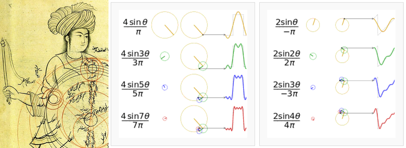
Figure 6.1: Epicycles and the Fourier series. Left: A demonstration of Mercury’s epicycles relative to the “center of the world” by Qutb al-Din al-Shirazi (1236 – 1311 A.D.) retrieved from Wikipedia. Middle and Right: How adding more epicycles (or terms in the Fourier series) will approximate functions. The right animation is also available.
Like most aspects of mathematics, this process of interpreting everything in terms of circles, began for astronomical purposes. When astronomers noticed that the orbit of Mars and other outer planets, did not appear to be a simple circle (as everything should have been in the heavens). At some point during their orbit, the revolution of these planets would become slower, stop, go back a little (in what is known as the retrograde motion) and then continue going forward again.
The correction proposed by Ptolemy (90 – 168 A.D.) was the most agreed upon. He put the planets on Epicycles or circles whose center itself rotates on a circle whose center is the earth. Eventually, as observations became more and more precise, it was necessary to add more and more epicycles in order to explain the complex motions of the planets180. Figure 6.1(Left) shows an example depiction of the epicycles of Mercury in the late 13th century.
Of course we now know that if they had abdicated the Earth from its throne in the center of the heavens and allowed the Sun to take its place, everything would become much simpler and true. But there was not enough observational evidence for changing the “professional consensus” of the time to this radical view suggested by a small minority181. So the pre-Galilean astronomers chose to keep Earth in the center and find a correction to the models (while keeping the heavens a purely “circular” order).
The main reason we are giving this historical background which might appear off topic is to give historical evidence that while such “approximations” do work and are very useful for pragmatic reasons (like measuring the calendar from the movement of astronomical bodies). They offer no physical insight. The astronomers who were involved with the Ptolemaic world view had to add a huge number of epicycles during the centuries after Ptolemy in order to explain more accurate observations. Finally the death knell of this world-view was Galileo’s observations with his new instrument (the telescope). So the physical insight, which is what Astronomers and Physicists are interested in (as opposed to Mathematicians and Engineers who just like proving and optimizing or calculating!) comes from being creative and not limiting ourselves to such approximations. Even when they work.
6.3.2.2 Circles and the complex plane 
Before going onto the derivation, it is also useful to review how the complex numbers and their plane relate to the circles we talked about above. The two schematics in the middle and right of Figure 6.1 show how a 1D function of time can be made using the 2D real and imaginary surface. Seeing the animation in Wikipedia will really help in understanding this important concept. At each point in time, we take the vertical coordinate of the point and use it to find the value of the function at that point in time. Figure 6.2 shows this relation with the axes marked.
Leonhard Euler182 (1707 – 1783 A.D.) showed that the complex exponential (\(e^{iv}\) where \(v\) is real) is periodic and can be written as: \(e^{iv}=\cos{v}+isin{v}\). Therefore \(e^{iv+2\pi}=e^{iv}\). Later, Caspar Wessel (mathematician and cartographer 1745 – 1818 A.D.) showed how complex numbers can be displayed as vectors on a plane. Euler’s identity might seem counter intuitive at first, so we will try to explain it geometrically (for deeper physical insight). On the real-imaginary 2D plane (like the left hand plot in each box of Figure 6.2), multiplying a number by \(i\) can be interpreted as rotating the point by \(90\) degrees (for example, the value \(3\) on the real axis becomes \(3i\) on the imaginary axis). On the other hand, \(e\equiv\lim_{n\rightarrow\infty}(1+{1\over n})^n\), therefore, defining \(m\equiv nu\), we get:
$$e^{u}=\lim_{n\rightarrow\infty}\left(1+{1\over n}\right)^{nu} =\lim_{n\rightarrow\infty}\left(1+{u\over nu}\right)^{nu} =\lim_{m\rightarrow\infty}\left(1+{u\over m}\right)^{m}$$
Taking \(u\equiv iv\) the result can be written as a generic complex number (a function of \(v\)):
$$e^{iv}=\lim_{m\rightarrow\infty}\left(1+i{v\over m}\right)^{m}=a(v)+ib(v)$$
For \(v=\pi\), a nice geometric animation of going to the limit can be seen on Wikipedia. We see that \(\lim_{m\rightarrow\infty}a(\pi)=-1\), while \(\lim_{m\rightarrow\infty}b(\pi)=0\), which gives the famous \(e^{i\pi}=-1\) equation. The final value is the real number \(-1\), however the distance of the polygon points traversed as \(m\rightarrow\infty\) is half the circumference of a circle or \(\pi\), showing how \(v\) in the equation above can be interpreted as an angle in units of radians and therefore how \(a(v)=cos(v)\) and \(b(v)=sin(v)\).
Since \(e^{iv}\) is periodic (let’s assume with a period of \(T\)), it is more clear to write it as \(v\equiv{2{\pi}n\over T}t\) (where \(n\) is an integer), so \(e^{iv}=e^{i{2{\pi}n\over T}t}\). The advantage of this notation is that the period (\(T\)) is clearly visible and the frequency (\(2{\pi}n \over T\), in units of 1/cycle) is defined through the integer \(n\). In this notation, \(t\) is in units of “cycle”s.
As we see from the examples in Figure 6.1 and Figure 6.2, for each constituting frequency, we need a respective ‘magnitude’ or the radius of the circle in order to accurately approximate the desired 1D function. The concepts of “period” and “frequency” are relatively easy to grasp when using temporal units like time because this is how we define them in every-day life. However, in an image (astronomical data), we are dealing with spatial units like distance. Therefore, by one “period” we mean the distance at which the signal is identical and frequency is defined as the inverse of that spatial “period”. The complex circle of Figure 6.2 can be thought of the Moon rotating about Earth which is rotating around the Sun; so the “Real (signal)” axis shows the Moon’s position as seen by a distant observer on the Sun as time goes by. Because of the scalar (not having any direction or vector) nature of time, Figure 6.2 is easier to understand in units of time. When thinking about spatial units, mentally replace the “Time (sec)” axis with “Distance (meters)”. Because length has direction and is a vector, visualizing the rotation of the imaginary circle and the advance along the “Distance (meters)” axis is not as simple as temporal units like time.
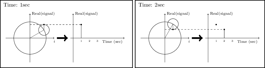
Figure 6.2: Relation between the real (signal), imaginary (\(i\equiv\sqrt{-1}\)) and time axes at two snapshots of time.
6.3.2.3 Fourier series 
In astronomical images, our variable (brightness, or number of photo-electrons, or signal to be more generic) is recorded over the 2D spatial surface of a camera pixel. However to make things easier to understand, here we will assume that the signal is recorded in 1D (assume one row of the 2D image pixels). Also for this section and the next (Fourier transform) we will be talking about the signal before it is digitized or pixelated. Let’s assume that we have the continuous function \(f(l)\) which is integrable in the interval \([l_0, l_0+L]\) (always true in practical cases like images). Take \(l_0\) as the position of the first pixel in the assumed row of the image and \(L\) as the width of the image along that row. The units of \(l_0\) and \(L\) can be in any spatial units (for example, meters) or an angular unit (like radians) multiplied by a fixed distance which is more common.
To approximate \(f(l)\) over this interval, we need to find a set of frequencies and their corresponding ‘magnitude’s (see Circles and the complex plane). Therefore our aim is to show \(f(l)\) as the following sum of periodic functions:
$$f(l)=\displaystyle\sum_{n=-\infty}^{\infty}c_ne^{i{2{\pi}n\over L}l} $$
Note that the different frequencies (\(2{\pi}n/L\), in units of cycles per meters for example) are not arbitrary. They are all integer multiples of the fundamental frequency of \(\omega_0=2\pi/L\). Recall that \(L\) was the length of the signal we want to model. Therefore, we see that the smallest possible frequency (or the frequency resolution) in the end, depends on the length we observed the signal or \(L\). In the case of each dimension on an image, this is the size of the image in the respective dimension. The frequencies have been defined in this “harmonic” fashion to insure that the final sum is periodic outside of the \([l_0, l_0+L]\) interval too. At this point, you might be thinking that the sky is not periodic with the same period as my camera’s view angle. You are absolutely right! The important thing is that since your camera’s observed region is the only region we are “observing” and will be using, the rest of the sky is irrelevant; so we can safely assume the sky is periodic outside of it. However, this working assumption will haunt us later in Edges in the frequency domain.
The frequencies are thus determined by definition. So all we need to do is to find the coefficients (\(c_n\)), or magnitudes, or radii of the circles for each frequency which is identified with the integer \(n\). Fourier’s approach was to multiply both sides with a fixed term:
$$f(l)e^{-i{2{\pi}m\over L}l}=\displaystyle\sum_{n=-\infty}^{\infty}c_ne^{i{2{\pi}(n-m)\over L}l} $$
where \(m>0\)183. We can then integrate both sides over the observation period:
$$\int_{l_0}^{l_0+L}f(l)e^{-i{2{\pi}m\over L}l}dl =\int_{l_0}^{l_0+L}\displaystyle\sum_{n=-\infty}^{\infty}c_ne^{i{2{\pi}(n-m)\over L}l}dl=\displaystyle\sum_{n=-\infty}^{\infty}c_n\int_{l_0}^{l_0+L}e^{i{2{\pi}(n-m)\over L}l}dl $$
Both \(n\) and \(m\) are positive integers. Also, we know that a complex exponential is periodic so after one period (\(L\)) it comes back to its starting point. Therefore \(\int_{l_0}^{l_0+L}e^{2{\pi}k/L}dl=0\) for any \(k>0\). However, when \(k=0\), this integral becomes: \(\int_{l_0}^{l_0+T}e^0dt=\int_{l_0}^{l_0+T}dt=T\). Hence since the integral will be zero for all \(n{\neq}m\), we get:
$$\displaystyle\sum_{n=-\infty}^{\infty}c_n\int_{l_0}^{l_0+T}e^{i{2{\pi}(n-m)\over L}l}dl=Lc_m $$
The origin of the axis is fundamentally an arbitrary position. So let’s set it to the start of the image such that \(l_0=0\). So we can find the “magnitude” of the frequency \(2{\pi}m/L\) within \(f(l)\) through the relation:
$$c_m={1\over L}\int_{0}^{L}f(l)e^{-i{2{\pi}m\over L}l}dl $$
6.3.2.4 Fourier transform 
In Fourier series, we had to assume that the function is periodic outside of the desired interval with a period of \(L\). Therefore, assuming that \(L\rightarrow\infty\) will allow us to work with any function. However, with this approximation, the fundamental frequency (\(\omega_0\)) or the frequency resolution that we discussed in Fourier series will tend to zero: \(\omega_0\rightarrow0\). In the equation to find \(c_m\), every \(m\) represented a frequency (multiple of \(\omega_0\)) and the integration on \(l\) removes the dependence of the right side of the equation on \(l\), making it only a function of \(m\) or frequency. Let’s define the following two variables:
$$\omega{\equiv}m\omega_0={2{\pi}m\over L}$$
$$F(\omega){\equiv}Lc_m$$
The equation to find the coefficients of each frequency in Fourier series thus becomes:
$$F(\omega)=\int_{-\infty}^{\infty}f(l)e^{-i{\omega}l}dl.$$
The function \(F(\omega)\) is thus the Fourier transform of \(f(l)\) in the frequency domain. So through this transformation, we can find (analyze) the magnitudes of the constituting frequencies or the value in the frequency space184 of our spatial input function. The great thing is that we can also do the reverse and later synthesize the input function from its Fourier transform. Let’s do it: with the approximations above, multiply the right side of the definition of the Fourier Series (Fourier series) with \(1=L/L=({\omega_0}L)/(2\pi)\):
$$f(l)={1\over 2\pi}\displaystyle\sum_{n=-\infty}^{\infty}Lc_ne^{{2{\pi}in\over L}l}\omega_0={1\over 2\pi}\displaystyle\sum_{n=-\infty}^{\infty}F(\omega)e^{i{\omega}l}\Delta\omega $$
To find the right most side of this equation, we renamed \(\omega_0\) as \(\Delta\omega\) because it was our resolution, \(2{\pi}n/L\) was written as \(\omega\) and finally, \(Lc_n\) was written as \(F(\omega)\) as we defined above. Now, as \(L\rightarrow\infty\), \(\Delta\omega\rightarrow0\) so we can write:
$$f(l)={1\over 2\pi}\int_{-\infty}^{\infty}F(\omega)e^{i{\omega}l}d\omega $$
Together, these two equations provide us with a very powerful set of tools that we can use to process (analyze) and recreate (synthesize) the input signal. Through the first equation, we can break up our input function into its constituent frequencies and analyze it, hence it is also known as analysis. Using the second equation, we can synthesize or make the input function from the known frequencies and their magnitudes. Thus it is known as synthesis. Here, we symbolize the Fourier transform (analysis) and its inverse (synthesis) of a function \(f(l)\) and its Fourier Transform \(F(\omega)\) as \({\cal F}[f]\) and \({\cal F}^{-1}[F]\).
6.3.2.5 Dirac delta and comb 
The Dirac \(\delta\) (delta) function (also known as an impulse) is the way that we convert a continuous function into a discrete one. It is defined to satisfy the following integral:
$$\int_{-\infty}^{\infty}\delta(l)dl=1$$
When integrated with another function, it gives that function’s value at \(l=0\):
$$\int_{-\infty}^{\infty}f(l)\delta(l)dt=f(0)$$
An impulse positioned at another point (say \(l_0\)) is written as \(\delta(l-l_0)\):
$$\int_{-\infty}^{\infty}f(l)\delta(l-l_0)dt=f(l_0)$$
The Dirac \(\delta\) function also operates similarly if we use summations instead of integrals. The Fourier transform of the delta function is:
$${\cal F}[\delta(l)]=\int_{-\infty}^{\infty}\delta(l)e^{-i{\omega}l}dl=e^{-i{\omega}0}=1$$
$${\cal F}[\delta(l-l_0)]=\int_{-\infty}^{\infty}\delta(l-l_0)e^{-i{\omega}l}dl=e^{-i{\omega}l_0}$$
From the definition of the Dirac \(\delta\) we can also define a Dirac comb (\({\rm III}_P\)) or an impulse train with infinite impulses separated by \(P\):
$${\rm III}_P(l)\equiv\displaystyle\sum_{k=-\infty}^{\infty}\delta(l-kP) $$
\(P\) is chosen to represent “pixel width” later in Sampling theorem. Therefore the Dirac comb is periodic with a period of \(P\). We have intentionally used a different name for the period of the Dirac comb compared to the input signal’s length of observation that we showed with \(L\) in Fourier series. This difference is highlighted here to avoid confusion later when these two periods are needed together in Discrete Fourier transform. The Fourier transform of the Dirac comb will be necessary in Sampling theorem, so let’s derive it. By its definition, it is periodic, with a period of \(P\), so the Fourier coefficients of its Fourier Series (Fourier series) can be calculated within one period:
$${\rm III}_P=\displaystyle\sum_{n=-\infty}^{\infty}c_ne^{i{2{\pi}n\over P}l}$$
We can now find the \(c_n\) from Fourier series:
$$c_n={1\over P}\int_{-P/2}^{P/2}\delta(l)e^{-i{2{\pi}n\over P}l} ={1\over P}\quad\quad \rightarrow \quad\quad {\rm III}_P={1\over P}\displaystyle\sum_{n=-\infty}^{\infty}e^{i{2{\pi}n\over P}l} $$
So we can write the Fourier transform of the Dirac comb as:
$${\cal F}[{\rm III}_P]=\int_{-\infty}^{\infty}{\rm III}_Pe^{-i{\omega}l}dl ={1\over P}\displaystyle\sum_{n=-\infty}^{\infty}\int_{-\infty}^{\infty}e^{-i(\omega-{2{\pi}n\over P})l}dl={1\over P}\displaystyle\sum_{n=-\infty}^{\infty}\delta\left(\omega-{2{\pi}n\over P}\right) $$
In the last step, we used the fact that the complex exponential is a periodic function, that \(n\) is an integer and that as we defined in Fourier transform, \(\omega{\equiv}m\omega_0\), where \(m\) was an integer. The integral will be zero for any \(\omega\) that is not equal to \(2{\pi}n/P\), a more complete explanation can be seen in Fourier series. Therefore, while in the spatial domain the impulses had spacing of \(P\) (meters for example), in the frequency space, the spacing between the different impulses are \(2\pi/P\) cycles per meters.
6.3.2.6 Convolution theorem 
The convolution (shown with the \(\ast\) operator) of the two functions \(f(l)\) and \(h(l)\) is defined as:
$$c(l)\equiv[f{\ast}h](l)=\int_{-\infty}^{\infty}f(\tau)h(l-\tau)d\tau $$
See Convolution process for a more detailed physical (pixel based) interpretation of this definition. The Fourier transform of convolution (\(C(\omega)\)) can be written as:
$$ C(\omega)=\int_{-\infty}^{\infty}[f{\ast}h](l)e^{-i{\omega}l}dl= \int_{-\infty}^{\infty}f(\tau)\left[\int_{-\infty}^{\infty}h(l-\tau)e^{-i{\omega}l}dl\right]d\tau $$
To solve the inner integral, let’s define \(s{\equiv}l-\tau\), so that \(ds=dl\) and \(l=s+\tau\) then the inner integral becomes:
$$\int_{-\infty}^{\infty}h(l-\tau)e^{-i{\omega}l}dl= \int_{-\infty}^{\infty}h(s)e^{-i{\omega}(s+\tau)}ds=e^{-i{\omega}\tau}\int_{-\infty}^{\infty}h(s)e^{-i{\omega}s}ds=H(\omega)e^{-i{\omega}\tau} $$
where \(H(\omega)\) is the Fourier transform of \(h(l)\). Substituting this result for the inner integral above, we get:
$$C(\omega)=H(\omega)\int_{-\infty}^{\infty}f(\tau)e^{-i{\omega}\tau}d\tau=H(\omega)F(\omega)=F(\omega)H(\omega) $$
where \(F(\omega)\) is the Fourier transform of \(f(l)\). So multiplying the Fourier transform of two functions individually, we get the Fourier transform of their convolution. The convolution theorem also proves a relation between the convolutions in the frequency space. Let’s define:
$$D(\omega){\equiv}F(\omega){\ast}H(\omega)$$
Applying the inverse Fourier Transform or synthesis equation (Fourier transform) to both sides and following the same steps above, we get:
$$d(l)=f(l)h(l)$$
Where \(d(l)\) is the inverse Fourier transform of \(D(\omega)\). We can therefore re-write the two equations above formally as the convolution theorem:
$$ {\cal F}[f{\ast}h]={\cal F}[f]{\cal F}[h] $$
$$ {\cal F}[fh]={\cal F}[f]\ast{\cal F}[h] $$
Besides its usefulness in blurring an image by convolving it with a given kernel, the convolution theorem also enables us to do another very useful operation in data analysis: to match the blur (or PSF) between two images taken with different telescopes/cameras or under different atmospheric conditions. This process is also known as deconvolution. Let’s take \(f(l)\) as the image with a narrower PSF (less blurry) and \(c(l)\) as the image with a wider PSF which appears more blurred. Also let’s take \(h(l)\) to represent the kernel that should be convolved with the sharper image to create the more blurry image. Above, we proved the relation between these three images through the convolution theorem. But there, we assumed that \(f(l)\) and \(h(l)\) are known (given) and the convolved image is desired.
In deconvolution, we have \(f(l)\) –the sharper image– and \(f*h(l)\) –the more blurry image– and we want to find the kernel \(h(l)\). The solution is a direct result of the convolution theorem:
$$ {\cal F}[h]={{\cal F}[f{\ast}h]\over {\cal F}[f]} \quad\quad {\rm or} \quad\quad h(l)={\cal F}^{-1}\left[{{\cal F}[f{\ast}h]\over {\cal F}[f]}\right] $$
While this works really nice, it has two problems:
- If \({\cal F}[f]\) has any zero values, then the inverse Fourier transform will not be a number!
- If there is significant noise in the image, then the high frequencies of the noise are going to significantly reduce the quality of the final result.
A standard solution to both these problems is the Weiner deconvolution algorithm185.
6.3.2.7 Sampling theorem 
Our mathematical functions are continuous, however, our data collecting and measuring tools are discrete. Here we want to give a mathematical formulation for digitizing the continuous mathematical functions so that later, we can retrieve the continuous function from the digitized recorded input. Assuming that we have a continuous function \(f(l)\), then we can define \(f_s(l)\) as the ‘sampled’ \(f(l)\) through the Dirac comb (see Dirac delta and comb):
$$f_s(l)=f(l){\rm III}_P=\displaystyle\sum_{n=-\infty}^{\infty}f(l)\delta(l-nP) $$
The discrete data-element \(f_k\) (for example, a pixel in an image), where \(k\) is an integer, can thus be represented as:
$$f_k=\int_{-\infty}^{\infty}f_s(l)dl=\int_{-\infty}^{\infty}f(l)\delta(l-kP)dt=f(kP)$$
Note that in practice, our discrete data points are not found in this fashion. Each detector pixel (in an image for example) has an area and averages the signal it receives over that area, not a mathematical point as the Dirac \(\delta\) function defines. However, as long as the variation in the signal over one detector pixel is not significant, this can be a good approximation. Having put this issue to the side, we can now try to find the relation between the Fourier transforms of the un-sampled \(f(l)\) and the sampled \(f_s(l)\). For a more clear notation, let’s define:
$$F_s(\omega)\equiv{\cal F}[f_s]$$
$$D(\omega)\equiv{\cal F}[{\rm III}_P]$$
Then using the Convolution theorem (see Convolution theorem), \(F_s(\omega)\) can be written as:
$$F_s(\omega)={\cal F}[f(l){\rm III}_P]=F(\omega){\ast}D(\omega)$$
Finally, from the definition of convolution and the Fourier transform of the Dirac comb (see Dirac delta and comb), we get:
$$\eqalign{ F_s(\omega) &= \int_{-\infty}^{\infty}F(\omega)D(\omega-\mu)d\mu \cr &= {1\over P}\displaystyle\sum_{n=-\infty}^{\infty}\int_{-\infty}^{\infty}F(\omega)\delta\left(\omega-\mu-{2{\pi}n\over P}\right)d\mu \cr &= {1\over P}\displaystyle\sum_{n=-\infty}^{\infty}F\left( \omega-{2{\pi}n\over P}\right).\cr } $$
\(F(\omega)\) was only a simple function, see Figure 6.3(left). However, from the sampled Fourier transform function we see that \(F_s(\omega)\) is the superposition of infinite copies of \(F(\omega)\) that have been shifted, see Figure 6.3(right). From the equation, it is clear that the shift in each copy is \(2\pi/P\).
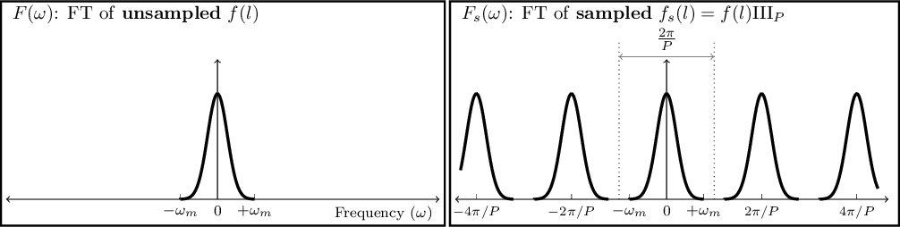
Figure 6.3: Sampling causes infinite repetition in the frequency domain. FT is an abbreviation for ‘Fourier transform’. \(\omega_m\) represents the maximum frequency present in the input. \(F(\omega)\) is only symmetric on both sides of 0 when the input is real (not complex). In general \(F(\omega)\) is complex and thus cannot be simply plotted like this. Here we have assumed a real Gaussian \(f(t)\) which has produced a Gaussian \(F(\omega)\).
The input \(f(l)\) can have any distribution of frequencies in it. In the example of Figure 6.3(left), the input consisted of a range of frequencies equal to \(\Delta\omega=2\omega_m\). Fortunately as Figure 6.3(right) shows, the assumed pixel size (\(P\)) we used to sample this hypothetical function was such that \(2\pi/P>\Delta\omega\). The consequence is that each copy of \(F(\omega)\) has become completely separate from the surrounding copies. Such a digitized (sampled) data set is thus called over-sampled. When \(2\pi/P=\Delta\omega\), \(P\) is just small enough to finely separate even the largest frequencies in the input signal and thus it is known as critically-sampled. Finally if \(2\pi/P<\Delta\omega\) we are dealing with an under-sampled data set. In an under-sampled data set, the separate copies of \(F(\omega)\) are going to overlap and this will deprive us of recovering high constituent frequencies of \(f(l)\). The effects of under-sampling in an image with high rates of change (for example, a brick wall imaged from a distance) can clearly be visually seen and is known as aliasing.
When the input \(f(l)\) is composed of a finite range of frequencies, \(f(l)\) is known as a band-limited function. The example in Figure 6.3(left) was a nice demonstration of such a case: for all \(\omega<-\omega_m\) or \(\omega>\omega_m\), we have \(F(\omega)=0\). Therefore, when the input function is band-limited and our detector’s pixels are placed such that we have critically (or over-) sampled it, then we can exactly reproduce the continuous \(f(l)\) from the discrete or digitized samples. To do that, we just have to isolate one copy of \(F(\omega)\) from the infinite copies and take its inverse Fourier transform.
This ability to exactly reproduce the continuous input from the sampled or digitized data leads us to the sampling theorem which connects the inherent property of the continuous signal (its maximum frequency) to that of the detector (the spacing between its pixels). The sampling theorem states that the full (continuous) signal can be recovered when the pixel size (\(P\)) and the maximum constituent frequency in the signal (\(\omega_m\)) have the following relation186:
$${2\pi\over P}>2\omega_m$$
This relation was first formulated by Harry Nyquist (1889 – 1976 A.D.) in 1928 and formally proved in 1949 by Claude E. Shannon (1916 – 2001 A.D.) in what is now known as the Nyquist-Shannon sampling theorem. In signal processing, the signal is produced (synthesized) by a transmitter and is received and de-coded (analyzed) by a receiver. Therefore producing a band-limited signal is necessary.
In astronomy, we do not produce the shapes of our targets, we are only observers. Galaxies can have any shape and size, therefore ideally, our signal is not band-limited. However, since we are always confined to observing through an aperture, the aperture will cause a point source (for which \(\omega_m=\infty\)) to be spread over several pixels. This spread is quantitatively known as the point spread function or PSF. This spread does blur the image which is undesirable; however, for this analysis it produces the positive outcome that there will be a finite \(\omega_m\). Though we should caution that any detector will have noise which will add lots of very high frequency (ideally infinite) changes between the pixels. However, the coefficients of those noise frequencies are usually exceedingly small.
6.3.2.8 Discrete Fourier transform 
As we have stated several times so far, the input image is a digitized, pixelated or discrete array of values (\(f_s(l)\), see Sampling theorem). The input is not a continuous function. Also, all our numerical calculations can only be done on a sampled, or discrete Fourier transform. Note that \(F_s(\omega)\) is not discrete, it is continuous. One way would be to find the analytic \(F_s(\omega)\), then sample it at any desired “freq-pixel”187 spacing. However, this process would involve two steps of operations and computers in particular are not too good at analytic operations for the first step. So here, we will derive a method to directly find the ‘freq-pixel’ated \(F_s(\omega)\) from the pixelated \(f_s(l)\). Let’s start with the definition of the Fourier transform (see Fourier transform):
$$F_s(\omega)=\int_{-\infty}^{\infty}f_s(l)e^{-i{\omega}l}dl $$
From the definition of \(f_s(\omega)\) (using \(x\) instead of \(n\)) we get:
$$\eqalign{ F_s(\omega) &= \displaystyle\sum_{x=-\infty}^{\infty} \int_{-\infty}^{\infty}f(l)\delta(l-xP)e^{-i{\omega}l}dl \cr &= \displaystyle\sum_{x=-\infty}^{\infty} f_xe^{-i{\omega}xP} } $$
Where \(f_x\) is the value of \(f(l)\) on the point \(x\) or the value of the \(x\)th pixel. As shown in Sampling theorem this function is infinitely periodic with a period of \(2\pi/P\). So all we need is the values within one period: \(0<\omega<2\pi/P\), see Figure 6.3. We want \(X\) samples within this interval, so the frequency difference between each frequency sample or freq-pixel is \(1/XP\). Hence we will evaluate the equation above on the points at:
$$\omega={u\over XP} \quad\quad u = 0, 1, 2, ..., X-1$$
Therefore the value of the freq-pixel \(u\) in the frequency domain is:
$$F_u=\displaystyle\sum_{x=0}^{X-1} f_xe^{-i{ux\over X}} $$
Therefore, we see that for each freq-pixel in the frequency domain, we are going to need all the pixels in the spatial domain188. If the input (spatial) pixel row is also \(X\) pixels wide, then we can exactly recover the \(x\)th pixel with the following summation:
$$f_x={1\over X}\displaystyle\sum_{u=0}^{X-1} F_ue^{i{ux\over X}} $$
When the input pixel row (we are still only working on 1D data) has \(X\) pixels, then it is \(L=XP\) spatial units wide. \(L\), or the length of the input data was defined in Fourier series and \(P\) or the space between the pixels in the input was defined in Dirac delta and comb. As we saw in Sampling theorem, the input (spatial) pixel spacing (\(P\)) specifies the range of frequencies that can be studied and in Fourier series we saw that the length of the (spatial) input, (\(L\)) determines the resolution (or size of the freq-pixels) in our discrete Fourier transformed image. Both result from the fact that the frequency domain is the inverse of the spatial domain.
6.3.2.9 Fourier operations in two dimensions 
Once all the relations in the previous sections have been clearly understood in one dimension, it is very easy to generalize them to two or even more dimensions since each dimension is by definition independent. Previously we defined \(l\) as the continuous variable in 1D and the inverse of the period in its direction to be \(\omega\). Let’s show the second spatial direction with \(m\) the inverse of the period in the second dimension with \(\nu\). The Fourier transform in 2D (see Fourier transform) can be written as:
$$F(\omega, \nu)=\int_{-\infty}^{\infty}\int_{-\infty}^{\infty} f(l, m)e^{-i({\omega}l+{\nu}m)}dl$$
$$f(l, m)=\int_{-\infty}^{\infty}\int_{-\infty}^{\infty} F(\omega, \nu)e^{i({\omega}l+{\nu}m)}dl$$
The 2D Dirac \(\delta(l,m)\) is non-zero only when \(l=m=0\). The 2D Dirac comb (or Dirac brush! See Dirac delta and comb) can be written in units of the 2D Dirac \(\delta\). For most image detectors, the sides of a pixel are equal in both dimensions. So \(P\) remains unchanged, if a specific device is used which has non-square pixels, then for each dimension a different value should be used.
$${\rm III}_P(l, m)\equiv\displaystyle\sum_{j=-\infty}^{\infty} \displaystyle\sum_{k=-\infty}^{\infty} \delta(l-jP, m-kP) $$
The Two dimensional Sampling theorem (see Sampling theorem) is thus very easily derived as before since the frequencies in each dimension are independent. Let’s take \(\nu_m\) as the maximum frequency along the second dimension. Therefore the two dimensional sampling theorem says that a 2D band-limited function can be recovered when the following conditions hold189:
$${2\pi\over P} > 2\omega_m \quad\quad\quad {\rm and} \quad\quad\quad {2\pi\over P} > 2\nu_m$$
Finally, let’s represent the pixel counter on the second dimension in the spatial and frequency domains with \(y\) and \(v\) respectively. Also let’s assume that the input image has \(Y\) pixels on the second dimension. Then the two dimensional discrete Fourier transform and its inverse (see Discrete Fourier transform) can be written as:
$$F_{u,v}=\displaystyle\sum_{x=0}^{X-1}\displaystyle\sum_{y=0}^{Y-1} f_{x,y}e^{-i({ux\over X}+{vy\over Y})} $$
$$f_{x,y}={1\over XY}\displaystyle\sum_{u=0}^{X-1}\displaystyle\sum_{v=0}^{Y-1} F_{u,v}e^{i({ux\over X}+{vy\over Y})} $$
6.3.2.10 Edges in the frequency domain 
With a good grasp of the frequency domain, we can revisit the problem of convolution on the image edges, see Edges in the spatial domain. When we apply the convolution theorem (see Convolution theorem) to convolve an image, we first take the discrete Fourier transforms (DFT, Discrete Fourier transform) of both the input image and the kernel, then we multiply them with each other and then take the inverse DFT to construct the convolved image. Of course, in order to multiply them with each other in the frequency domain, the two images have to be the same size, so let’s assume that we pad the kernel (it is usually smaller than the input image) with zero valued pixels in both dimensions so it becomes the same size as the input image before the DFT.
Having multiplied the two DFTs, we now apply the inverse DFT which is where the problem is usually created. If the DFT of the kernel only had values of 1 (unrealistic condition!) then there would be no problem and the inverse DFT of the multiplication would be identical with the input. However in real situations, the kernel’s DFT has a maximum of 1 (because the sum of the kernel has to be one, see Convolution process) and decreases something like the hypothetical profile of Figure 6.3. So when multiplied with the input image’s DFT, the coefficients or magnitudes (see Circles and the complex plane) of the smallest frequency (or the sum of the input image pixels) remains unchanged, while the magnitudes of the higher frequencies are significantly reduced.
As we saw in Sampling theorem, the Fourier transform of a discrete input will be infinitely repeated. In the final inverse DFT step, the input is in the frequency domain (the multiplied DFT of the input image and the kernel DFT). So the result (our output convolved image) will be infinitely repeated in the spatial domain. In order to accurately reconstruct the input image, we need all the frequencies with the correct magnitudes. However, when the magnitudes of higher frequencies are decreased, longer periods (shorter frequencies) will dominate in the reconstructed pixel values. Therefore, when constructing a pixel on the edge of the image, the newly empowered longer periods will look beyond the input image edges and will find the repeated input image there. So if you convolve an image in this fashion using the convolution theorem, when a bright object exists on one edge of the image, its blurred wings will be present on the other side of the convolved image. This is often termed as circular convolution or cyclic convolution.
So, as long as we are dealing with convolution in the frequency domain, there is nothing we can do about the image edges. The least we can do is to eliminate the ghosts of the other side of the image. So, we add zero valued pixels to both the input image and the kernel in both dimensions so the image that will be convolved has a size equal to the sum of both images in each dimension. Of course, the effect of this zero-padding is that the sides of the output convolved image will become dark. To put it another way, the edges are going to drain the flux from nearby objects. But at least it is consistent across all the edges of the image and is predictable. In Convolve, you can see the padded images when inspecting the frequency domain convolution steps with the --viewfreqsteps option.
6.3.3 Spatial vs. Frequency domain 
With the discussions above it might not be clear when to choose the spatial domain and when to choose the frequency domain. Here we will try to list the benefits of each.
The spatial domain,
- Can correct for the edge effects of convolution, see Edges in the spatial domain.
- Can operate on blank pixels.
- Can be faster than frequency domain when the kernel is small (in terms of the number of pixels on the sides).
The frequency domain,
- Will be much faster when the image and kernel are both large.
As a general rule of thumb, when working on an image of modeled profiles use the frequency domain and when working on an image of real (observed) objects use the spatial domain (corrected for the edges). The reason is that if you apply a frequency domain convolution to a real image, you are going to loose information on the edges and generally you do not want large kernels. But when you have made the profiles in the image yourself, you can just make a larger input image and crop the central parts to completely remove the edge effect, see If convolving afterwards. Also due to oversampling, both the kernels and the images can become very large and the speed boost of frequency domain convolution will significantly improve the processing time, see Oversampling.
6.3.4 Convolution kernel 
All the programs that need convolution will need to be given a convolution kernel file and extension. In most cases (other than Convolve, see Convolve) the kernel file name is optional. However, the extension is necessary and must be specified either on the command-line or at least one of the configuration files (see Configuration files). Within Gnuastro, there are two ways to create a kernel image:
- MakeProfiles: You can use MakeProfiles to create a parametric (based on a radial function) kernel, see MakeProfiles. By default MakeProfiles will make the Gaussian and Moffat profiles in a separate file so you can feed it into any of the programs.
- ConvertType: You can write your own desired kernel into a text file table and convert it to a FITS file with ConvertType, see ConvertType. Just be careful that the kernel has to have an odd number of pixels along its two axes, see Convolution process. All the programs that do convolution will normalize the kernel internally, so if you choose this option, you do not have to worry about normalizing the kernel. Only within Convolve, there is an option to disable normalization, see Invoking Convolve.
The two options to specify a kernel file name and its extension are shown below. These are common between all the programs that will do convolution.
- -k FITS
- --kernel=FITS
The convolution kernel file name. The
BITPIX(data type) value of this file can be any standard type and it does not necessarily have to be normalized. Several operations will be done on the kernel image prior to the program’s processing:- It will be converted to floating point type.
- All blank pixels (see Blank pixels) will be set to zero.
- It will be normalized so the sum of its pixels equal unity.
- It will be flipped so the convolved image has the same orientation. This is only relevant if the kernel is not circular. See Convolution process.
- -U STR
- --khdu=STR
The convolution kernel HDU. Although the kernel file name is optional, before running any of the programs, they need to have a value for --khdu even if the default kernel is to be used. So be sure to keep its value in at least one of the configuration files (see Configuration files). By default, the system configuration file has a value.
6.3.5 Invoking Convolve 
Convolve an input dataset (2D image or 1D spectrum for example) with a known kernel, or make the kernel necessary to match two PSFs. The general template for Convolve is:
$ astconvolve [OPTION...] ASTRdata
One line examples:
## Convolve mockimg.fits with psf.fits:
$ astconvolve --kernel=psf.fits mockimg.fits
## Convolve in the spatial domain:
$ astconvolve observedimg.fits --kernel=psf.fits --domain=spatial
## Convolve a 3D cube (only spatial domain is supported in 3D).
## It is also necessary to define 3D tiles and channels for
## parallelization (see the Tessellation section for more).
$ astconvolve cube.fits --kernel=kernel3d.fits --domain=spatial \
--tilesize=30,30,30 --numchannels=1,1,1
## Find the kernel to convolve with a sharper PSF to become similar
## to a broader PSF (they both have to have the same pixel size).
$ astconvolve --kernel=sharper-psf.fits --makekernel=10 \
broader-psf.fits
## Convolve a Spectrum (column 14 in the FITS table below) with a
## custom kernel (the kernel will be normalized internally, so only
## the ratios are important). Sed is used to replace the spaces with
## new line characters so Convolve sees them as values in one column.
$ echo "1 3 10 3 1" | sed 's/ /\n/g' | astconvolve spectra.fits -c14
The only argument accepted by Convolve is an input image file. Some of the options are the same between Convolve and some other Gnuastro programs. Therefore, to avoid repetition, they will not be repeated here. For the full list of options shared by all Gnuastro programs, please see Common options. In particular, in the spatial domain, on a multi-dimensional datasets, convolve uses Gnuastro’s tessellation to speed up the run, see Tessellation. Common options related to tessellation are described in Processing options.
1-dimensional datasets (for example, spectra) are only read as columns within a table (see Tables for more on how Gnuastro programs read tables). Note that currently 1D convolution is only implemented in the spatial domain and thus kernel-matching is also not supported.
Here we will only explain the options particular to Convolve. Run Convolve with --help in order to see the full list of options Convolve accepts, irrespective of where they are explained in this book.
- --kernelcolumn
Column containing the 1D kernel. When the input dataset is a 1-dimensional column, and the host table has more than one column, use this option to specify which column should be used.
- --nokernelflip
Do not flip the kernel after reading; only for spatial domain convolution. This can be useful if the flipping has already been applied to the kernel. By default, the input kernel is flipped to avoid the output getting flipped; see Convolution process.
- --nokernelnorm
Do not normalize the kernel after reading it, such that the sum of its pixels is unity. As described in Convolution process, the kernel is normalized by default.
- --conv-on-blank
Do not ignore blank pixels in the convolution. The output pixels that were originally non-blank are not affected by this option (they will have the same value if this option is called or not). This option just expands/dilates the non-blank regions of your dataset into the blank regions and only works in spatial domain convolution. Therefore, with this option convolution can be used as a proxy for interpolation or dilation.
By default, blank pixels are ignored during spatial domain convolution; so the input and output have exactly the same number of blank pixels. With this option, the blank pixels that are sufficiently close to non-blank pixels (based on the kernel) will be given a value based on the non-blank elements that overlap with the kernel for that blank pixel (see Edges in the spatial domain).
- -d STR 
- --domain=STR
The domain to use for the convolution. The acceptable values are ‘
spatial’ and ‘frequency’, corresponding to the respective domain.For large images, the frequency domain process will be more efficient than convolving in the spatial domain. However, the edges of the image will loose some flux (see Edges in the spatial domain) and the image must not contain any blank pixels, see Spatial vs. Frequency domain.
- --checkfreqsteps
With this option a file with the initial name of the output file will be created that is suffixed with _freqsteps.fits, all the steps done to arrive at the final convolved image are saved as extensions in this file. The extensions in order are:
- The padded input image. In frequency domain convolution the two images (input and convolved) have to be the same size and both should be padded by zeros.
- The padded kernel, similar to the above.
- The Fourier spectrum of the forward Fourier transform of the input image. Note that the Fourier transform is a complex operation (and not view able in one image!) So we either have to show the ‘Fourier spectrum’ or the ‘Phase angle’. For the complex number \(a+ib\), the Fourier spectrum is defined as \(\sqrt{a^2+b^2}\) while the phase angle is defined as \(\arctan(b/a)\).
- The Fourier spectrum of the forward Fourier transform of the kernel image.
- The Fourier spectrum of the multiplied (through complex arithmetic) transformed images.
- The inverse Fourier transform of the multiplied image. If you open it, you will see that the convolved image is now in the center, not on one side of the image as it started with (in the padded image of the first extension). If you are working on a mock image which originally had pixels of precisely 0.0, you will notice that in those parts that your convolved profile(s) did not convert, the values are now \(\sim10^{-18}\), this is due to floating-point round off errors. Therefore in the final step (when cropping the central parts of the image), we also remove any pixel with a value less than \(10^{-17}\).
- --noedgecorrection
Do not correct the edge effect in spatial domain convolution (this correction is done in spatial domain convolution by default). For a full discussion, please see Edges in the spatial domain.
- -m INT
- --makekernel=INT
If this option is called, Convolve will do PSF-matching: the output will be the kernel that you should convolve with the sharper image to obtain the blurry one (see Convolution theorem). The two images must have the same size (number of pixels). This option is not yet supported in 1-dimensional datasets. In effect, it is only necessary to give the two PSFs of your two datasets, find the matching kernel based on that, then apply that kernel to the higher-resolution (sharper image).
The image given to the --kernel option is assumed to be the sharper (less blurry) image and the input image (with no option) is assumed to be the more blurry image. The value given to this option will be used as the maximum radius of the kernel. Any pixel in the final kernel that is larger than this distance from the center will be set to zero.
Noise has large frequencies which can make the result less reliable for the higher frequencies of the final result. So all the frequencies which have a spectrum smaller than the value given to the minsharpspec option in the sharper input image are set to zero and not divided. This will cause the wings of the final kernel to be flatter than they would ideally be which will make the convolved image result unreliable if it is too high.
There is a complete tutorial in Gnuastro on how to build the (extended) PSF: Building the extended PSF. Since the very extended PSF wings can be subtracted before matching (as described in that tutorial), for PSF-matching, you may not need the full extended PSF. It it is good to validate how large the PSF to match should be, based on the size of the sources you want to study: if it is a large nearby galaxy, you need a larger PSF, but if it is high redshift galaxies, only the inner part of the tutorial above is enough.
- -c
- --minsharpspec
(=FLT) The minimum frequency spectrum (or coefficient, or pixel value in the frequency domain image) to use in deconvolution, see the explanations under the --makekernel option for more information.
6.4 Warp 
Image warping is the process of mapping the pixels of one image onto a new pixel grid. This process is sometimes known as transformation, however following the discussion of Heckbert 1989190 we will not be using that term because it can be confused with only pixel value or flux transformations. Here we specifically mean the pixel grid transformation which is better conveyed with ‘warp’.
Image warping is a very important step in astronomy, both in observational data analysis and in simulating modeled images. In modeling, warping an image is necessary when we want to apply grid transformations to the initial models, for example, in simulating gravitational lensing. Observational reasons for warping an image are listed below:
- Noise: Most scientifically interesting targets are inherently faint (have a very low Signal to noise ratio). Therefore one short exposure is not enough to detect such objects that are drowned deeply in the noise. We need multiple exposures so we can add them together and increase the objects’ signal to noise ratio. Keeping the telescope fixed on one field of the sky is practically impossible. Therefore very deep observations have to put into the same grid before adding them.
- Resolution: If we have multiple images of one patch of the sky (hopefully at multiple orientations) we can warp them to the same grid. The multiple orientations will allow us to ‘guess’ the values of pixels on an output pixel grid that has smaller pixel sizes and thus increase the resolution of the output. This process of merging multiple observations is known as Mosaicing.
- Cosmic rays: Cosmic rays can randomly fall on any part of an image. If they collide vertically with the camera, they are going to create a very sharp and bright spot that in most cases can be separated easily191. However, depending on the depth of the camera pixels, and the angle that a cosmic rays collides with it, it can cover a line-like larger area on the CCD which makes the detection using their sharp edges very hard and error prone. One of the best methods to remove cosmic rays is to compare multiple images of the same field. To do that, we need all the images to be on the same pixel grid.
- Optical distortion: In wide field images, the optical distortion that occurs on the outer parts of the focal plane will make accurate comparison of the objects at various locations impossible. It is therefore necessary to warp the image and correct for those distortions prior to the analysis.
- Detector not on focal plane: In some cases (like the Hubble Space Telescope ACS and WFC3 cameras), the CCD might be tilted compared to the focal plane, therefore the recorded CCD pixels have to be projected onto the focal plane before further analysis.
6.4.1 Linear warping basics 
Let’s take \(\left[\matrix{u&v}\right]\) as the coordinates of a point in the input image and \(\left[\matrix{x&y}\right]\) as the coordinates of that same point in the output image192. The simplest form of coordinate transformation (or warping) is the scaling of the coordinates, let’s assume we want to scale the first axis by \(M\) and the second by \(N\), the output coordinates of that point can be calculated by
$$\left[\matrix{x\cr y}\right]= \left[\matrix{Mu\cr Nv}\right]= \left[\matrix{M&0\cr0&N}\right]\left[\matrix{u\cr v}\right]$$
Note that these are matrix multiplications. We thus see that we can represent any such grid warping as a matrix. Another thing we can do with this \(2\times2\) matrix is to rotate the output coordinate around the common center of both coordinates. If the output is rotated anticlockwise by \(\theta\) degrees from the positive (to the right) horizontal axis, then the warping matrix should become:
$$\left[\matrix{x\cr y}\right]= \left[\matrix{ucos\theta-vsin\theta\cr usin\theta+vcos\theta}\right]= \left[\matrix{cos\theta&-sin\theta\cr sin\theta&cos\theta}\right] \left[\matrix{u\cr v}\right] $$
We can also flip the coordinates around the first axis, the second axis and the coordinate center with the following three matrices respectively:
$$\left[\matrix{1&0\cr0&-1}\right]\quad\quad \left[\matrix{-1&0\cr0&1}\right]\quad\quad \left[\matrix{-1&0\cr0&-1}\right]$$
The final thing we can do with this definition of a \(2\times2\) warping matrix is shear. If we want the output to be sheared along the first axis with \(A\) and along the second with \(B\), then we can use the matrix:
$$\left[\matrix{1&A\cr B&1}\right]$$
To have one matrix representing any combination of these steps, you use matrix multiplication, see Merging multiple warpings. So any combinations of these transformations can be displayed with one \(2\times2\) matrix:
$$\left[\matrix{a&b\cr c&d}\right]$$
The transformations above can cover a lot of the needs of most coordinate transformations. However they are limited to mapping the point \([\matrix{0&0}]\) to \([\matrix{0&0}]\). Therefore they are useless if you want one coordinate to be shifted compared to the other one. They are also space invariant, meaning that all the coordinates in the image will receive the same transformation. In other words, all the pixels in the output image will have the same area if placed over the input image. So transformations which require varying output pixel sizes like projections cannot be applied through this \(2\times2\) matrix either (for example, for the tilted ACS and WFC3 camera detectors on board the Hubble space telescope).
To add these further capabilities, namely translation and projection, we use the homogeneous coordinates. They were defined about 200 years ago by August Ferdinand Möbius (1790 – 1868). For simplicity, we will only discuss points on a 2D plane and avoid the complexities of higher dimensions. We cannot provide a deep mathematical introduction here, interested readers can get a more detailed explanation from Wikipedia193 and the references therein.
By adding an extra coordinate to a point we can add the flexibility we need. The point \([\matrix{x&y}]\) can be represented as \([\matrix{xZ&yZ&Z}]\) in homogeneous coordinates. Therefore multiplying all the coordinates of a point in the homogeneous coordinates with a constant will give the same point. Put another way, the point \([\matrix{x&y&Z}]\) corresponds to the point \([\matrix{x/Z&y/Z}]\) on the constant \(Z\) plane. Setting \(Z=1\), we get the input image plane, so \([\matrix{u&v&1}]\) corresponds to \([\matrix{u&v}]\). With this definition, the transformations above can be generally written as:
$$\left[\matrix{x\cr y\cr 1}\right]= \left[\matrix{a&b&0\cr c&d&0\cr 0&0&1}\right] \left[\matrix{u\cr v\cr 1}\right]$$
We thus acquired 4 extra degrees of freedom. By giving non-zero values to the zero valued elements of the last column we can have translation (try the matrix multiplication!). In general, any coordinate transformation that is represented by the matrix below is known as an affine transformation194:
$$\left[\matrix{a&b&c\cr d&e&f\cr 0&0&1}\right]$$
We can now consider translation, but the affine transform is still spatially invariant. Giving non-zero values to the other two elements in the matrix above gives us the projective transformation or Homography195 which is the most general type of transformation with the \(3\times3\) matrix:
$$\left[\matrix{x'\cr y'\cr w}\right]= \left[\matrix{a&b&c\cr d&e&f\cr g&h&1}\right] \left[\matrix{u\cr v\cr 1}\right]$$
So the output coordinates can be calculated from:
$$x={x' \over w}={au+bv+c \over gu+hv+1}\quad\quad\quad\quad y={y' \over w}={du+ev+f \over gu+hv+1}$$
Thus with Homography we can change the sizes of the output pixels on the input plane, giving a ‘perspective’-like visual impression. This can be quantitatively seen in the two equations above. When \(g=h=0\), the denominator is independent of \(u\) or \(v\) and thus we have spatial invariance. Homography preserves lines at all orientations. A very useful fact about Homography is that its inverse is also a Homography. These two properties play a very important role in the implementation of this transformation. A short but instructive and illustrated review of affine, projective and also bi-linear mappings is provided in Heckbert 1989196.
6.4.2 Merging multiple warpings 
In Linear warping basics we saw how a basic warp/transformation can be represented with a matrix. To make more complex warpings (for example, to define a translation, rotation and scale as one warp) the individual matrices have to be multiplied through matrix multiplication. However matrix multiplication is not commutative, so the order of the set of matrices you use for the multiplication is going to be very important.
The first warping should be placed as the left-most matrix. The second warping to the right of that and so on. The second transformation is going to occur on the warped coordinates of the first. As an example for merging a few transforms into one matrix, the multiplication below represents the rotation of an image about a point \([\matrix{U&V}]\) anticlockwise from the horizontal axis by an angle of \(\theta\). To do this, first we take the origin to \([\matrix{U&V}]\) through translation. Then we rotate the image, then we translate it back to where it was initially. These three operations can be merged in one operation by calculating the matrix multiplication below:
$$\left[\matrix{1&0&U\cr0&1&V\cr{}0&0&1}\right] \left[\matrix{cos\theta&-sin\theta&0\cr sin\theta&cos\theta&0\cr 0&0&1}\right] \left[\matrix{1&0&-U\cr0&1&-V\cr{}0&0&1}\right]$$
6.4.3 Resampling 
A digital image is composed of discrete ‘picture elements’ or ‘pixels’. When a real image is created from a camera or detector, each pixel’s area is used to store the number of photo-electrons that were created when incident photons collided with that pixel’s surface area. This process is called the ‘sampling’ of a continuous or analog data into digital data.
When we change the pixel grid of an image, or “warp” it, we have to calculate the flux value of each pixel on the new grid based on the old grid, or resample it. Because of the calculation (as opposed to observation), any form of warping on the data is going to degrade the image and mix the original pixel values with each other. So if an analysis can be done on an unwarped data image, it is best to leave the image untouched and pursue the analysis. However as discussed in Warp this is not possible in some scenarios and re-sampling is necessary.
When the FWHM of the PSF of the camera is much larger than the pixel scale (see Sampling theorem) we are sampling the signal in a much higher resolution than the camera can offer. This is usually the case in many applications of image processing (nonastronomical imaging). In such cases, we can consider each pixel to be a point and not an area: the PSF doesn’t vary much over a single pixel.
Approximating a pixel’s area to a point can significantly speed up the resampling and also the simplicity of the code. Because resampling becomes a problem of interpolation: points of the input grid need to be interpolated at certain other points (over the output grid). To increase the accuracy, you might also sample more than one point from within a pixel giving you more points for a more accurate interpolation in the output grid.
However, interpolation has several problems. The first one is that it will depend on the type of function you want to assume for the interpolation. For example, you can choose a bi-linear or bi-cubic (the ‘bi’s are for the 2 dimensional nature of the data) interpolation method. For the latter there are various ways to set the constants197. Such parametric interpolation functions can fail seriously on the edges of an image, or when there is a sharp change in value (for example, the bleeding saturation of bright stars in astronomical CCDs). They will also need normalization so that the flux of the objects before and after the warping is comparable.
The parametric nature of these methods adds a level of subjectivity to the data (it makes more assumptions through the functions than the data can handle). For most applications this is fine (as discussed above: when the PSF is over-sampled), but in scientific applications where we push our instruments to the limit and the aim is the detection of the faintest possible galaxies or fainter parts of bright galaxies, we cannot afford this loss. Because of these reasons Warp will not use parametric interpolation techniques.
Warp will do interpolation based on “pixel mixing”198 or “area resampling”. This is also similar to what the Hubble Space Telescope pipeline calls “Drizzling”199. This technique requires no functions, it is thus non-parametric. It is also the closest we can get (make least assumptions) to what actually happens on the detector pixels.
In pixel mixing, the basic idea is that you reverse-transform each output pixel to find which pixels of the input image it covers, and what fraction of the area of the input pixels are covered by that output pixel. We then multiply each input pixel’s value by the fraction of its area that overlaps with the output pixel (between 0 to 1). The output’s pixel value is derived by summing all these multiplications for the input pixels that it covers.
Through this process, pixels are treated as an area not as a point (which is how detectors create the image), also the brightness (see Brightness, Flux, Magnitude and Surface brightness) of an object will be fully preserved. Since it involves the mixing of the input’s pixel values, this pixel mixing method is a form of Spatial domain convolution. Therefore, after comparing the input and output, you will notice that the output is slightly smoothed, thus boosting the more diffuse signal, but creating correlated noise. In astronomical imaging the correlated noise will be decreased later when you coadd many exposures200.
If there are very high spatial-frequency signals in the image (for example, fringes) which vary on a scale smaller than your output image pixel size (this is rarely the case in astronomical imaging), pixel mixing can cause ailiasing201. Therefore, in case such fringes are present, they have to be calculated and removed separately (which would naturally be done in any astronomical reduction pipeline). Because of the PSF, no astronomical target has a sharp change in their signal. Thus this issue is less important for astronomical applications, see Point spread function.
To find the overlap area of the output pixel over the input pixels, we need to define polygons and clip them (find the overlap).
Usually, it is sufficient to define a pixel with a four-vertice polygon.
However, when a non-linear distortion (for example, SIP or TPV) is present and the distortion is significant over an output pixel’s size (usually far from the reference point), the shadow of the output pixel on the input grid can be curved.
To account for such cases (which can only happen when correcting for non-linear distortions), Warp has the --edgesampling option to sample the output pixel over more vertices.
For more, see the description of this option in Align pixels with WCS considering distortions.
6.4.4 Invoking Warp 
Warp will warp an input image into a new pixel grid by pixel mixing (see Resampling). Without any options, Warp will remove any non-linear distortions from the image and align the output pixel coordinates to its WCS coordinates. Any homographic warp (for example, scaling, rotation, translation, projection, see Linear warping basics) can also be done by calling the relevant option explicitly. The general template for invoking Warp is:
$ astwarp [OPTIONS...] InputImage
One line examples:
## Align image with celestial coordinates and remove any distortion
$ astwarp image.fits
## Align four exposures to same pixel grid and coadd them with
## Arithmetic program's sigma-clipped mean operator (out of many
## coadding operators, see Arithmetic's documentation).
$ grid="--center=1.234,5.678 --width=1001,1001 --widthinpix --cdelt=0.2/3600"
$ astwarp a.fits $grid --output=A.fits
$ astwarp b.fits $grid --output=B.fits
$ astwarp c.fits $grid --output=C.fits
$ astwarp d.fits $grid --output=D.fits
$ astarithmetic A.fits B.fits C.fits D.fits 4 5 0.2 sigclip-mean \
-g1 --writeall --output=coadd.fits
## Warp a previously created mock image to the same pixel grid as the
## real image (including any distortions).
$ astwarp mock.fits --gridfile=real.fits
## Rotate and then scale input image:
$ astwarp --rotate=37.92 --scale=0.8 image.fits
## Scale, then translate the input image:
$ astwarp --scale 8/3 --translate 2.1 image.fits
## Directly input a custom warping matrix (using fraction):
$ astwarp --matrix=1/5,0,4/10,0,1/5,4/10,0,0,1 image.fits
## Directly input a custom warping matrix, with final numbers:
$ astwarp --matrix="0.7071,-0.7071, 0.7071,0.7071" image.fits
If any processing is to be done, Warp needs to be given a 2D FITS image. As in all Gnuastro programs, when an output is not explicitly set with the --output option, the output filename will be set automatically based on the operation, see Automatic output. For the full list of general options to all Gnuastro programs (including Warp), please see Common options.
Warp uses pixel mixing to derive the pixel values of the output image, see Resampling. To be the most accurate, the input image will be read as a 64-bit double precision floating point dataset and all internal processing is done in this format. Upon writing, by default it will be converted to 32-bit single precision floating point type (actual observational data rarely have such precision!). In case you want a different output type, you can use the --type option that is common to several Gnuastro programs. For example, if your input is a mock image without noise, and you want to preserve the 64-bit precision, use (with --type=float64. Just note that the file size will also be double! For more on the precision of various types, see Numeric data types.
By default (if no linear operation is requested), Warp will align the pixel grid of the input image to the WCS coordinates it contains. This operation and the the options that govern it are described in Align pixels with WCS considering distortions. You can Warp an input image to the same pixel grid as a reference FITS file using the --wcsfile option. In this case, the output image will take all the information needed from the reference WCS file and HDU/extension specified with --wcshdu, thus it will discard any other resampling options given.
If you need any custom linear warping (independent of the WCS, see Linear warping basics), you need to call the respective operation manually. These are described in Linear warps to be called explicitly. Please note that you may not use both linear and non-linear modes simultaneously. For example, you cannot scale or rotate the image while removing its non-linear distortions at the same time.
The following options are shared between both modes:
- --hstartwcs=INT
Specify the first header keyword number (line) that should be used to read the WCS information, see the full explanation in Invoking Crop.
- --hendwcs=INT
Specify the last header keyword number (line) that should be used to read the WCS information, see the full explanation in Invoking Crop.
- -C FLT
- --coveredfrac=FLT
Depending on the warp, the output pixels that cover pixels on the edge of the input image, or blank pixels in the input image, are not going to be fully covered by input data. With this option, you can specify the acceptable covered fraction of such pixels (any value between 0 and 1). If you only want output pixels that are fully covered by the input image area (and are not blank), then you can set --coveredfrac=1 (which is the default!). Alternatively, a value of
0will keep output pixels that are even infinitesimally covered by the input. As a result, with --coveredfrac=0, the sum of the pixels in the input and output images will be exactly the same.
6.4.4.1 Align pixels with WCS considering distortions 
When none of the linear warps202 are requested, Warp will align the input’s pixel axes with it’s WCS axes.
In the process, any possibly existing distortion is also removed (such as TPV and SIP).
Usually, the WCS axes are the Right Ascension and Declination in equatorial coordinates.
The output image’s pixel grid is highly customizable through the options in this section.
To learn about Warp’s strategy to build the new pixel grid, see Resampling.
For strong distortions (that produce strong curvatures), you can fine-tune the area-based resampling with --edgesampling, as described below.
On the other hand, sometimes you need to Warp an input image to the exact same grid of an already available reference FITS image with an existing WCS. If that image is already aligned, finding its center, number of pixels and pixel scale can be annoying (and just increase the complexity of your script). On the other hand, if that image is not aligned (for example, has a certain rotation in the sky, and has a different distortion), there are too many WCS parameters to set (some are not yet available explicitly in the options here)! For such scenarios, Warp has the --gridfile option. When --gridfile is called, the options below that are used to define the output’s WCS will be ignored (these options: --center, --widthinpix, --cdelt, --ctype). In this case, the output’s WCS and pixel grid will exactly match the image given to --gridfile (including any rotation, pixel scale, or distortion or projection).
|
Set --cdelt explicitly when you plan to coadd many warped images: To align some images and later coadd them, it is necessary to be sure the pixel sizes of all the images are the same exactly. Most of the time the measured (during astrometry) pixel scale of the separate exposures, will be different in the second or third digit number after the decimal point. It is a normal/statistical error in measuring the astrometry. On a large image, these slight differences can cause different output sizes (of one or two pixels on a very large image). You can fix this by explicitly setting the pixel scale of each warped exposure with Warp’s --cdelt option that is described below. For good strategies of setting the pixel scale, see Moiré pattern in coadding and its correction. |
Another problem that may arise when aligning images to new pixel grids is the aliasing or visible Moiré patterns on the output image. This artifact should be removed if you are coadding several exposures, especially with a pointing pattern. If not see Moiré pattern in coadding and its correction for ways to mitigate the visible patterns. See the description of --gridfile below for more.
|
Known issue: Warp’s WCS-based aligning works best with WCSLIB version 7.12 (released in September 2022) and above.
If you have an older version of WCSLIB, you might get a |
- -c FLT,FLT 
- --center=FLT,FLT
WCS coordinates of the center of the central pixel of the output image. Since a central pixel is only defined with an odd number of pixels along both dimensions, the output will always have an odd number of pixels. When --center or --gridfile aren’t given, the output will have the same central WCS coordinate as the input.
Usually, the WCS coordinates are Right Ascension and Declination (when the first three characters of
CTYPE1andCTYPE2are respectivelyRA-andDEC). For more on theCTYPEikeyword values, see--ctypebelow.- -w INT[,INT]
- --width=INT[,INT]
Width and height of the output image in units of WCS (usually degrees). If you want the values to be read as pixels, also call the --widthinpix option with --width. If a single value is given, Warp will use the same value for the second dimension (creating a square output). When --width or --gridfile aren’t given, Warp will calculate the necessary size of the output pixel grid to fully contain the input image.
Usually the WCS coordinates are in units of degrees (defined by the
CUNITikeywords of the FITS standard). But entering a certain number of arcseconds or arcminutes for the width can be annoying (you will usually need to go to the calculator!). To simplify such situations, this option also accepts division. For example --width=1/60,2/60 will make an aligned warp that is 1 arcmin along Right Ascension and 2 arcminutes along the Declination.With the --widthinpix option the values will be interpreted as numbers of pixels. In this scenario, this option should be given odd integer(s) that are greater than 1. This ensures that the output image can have a central pixel. Recall that through the --center option, you specify the WCS coordinate of the center of the central pixel. The central coordinate of an image with an even number of pixels will be on the edge of two pixels, so a “central” pixel is not well defined. If any of the given values are even, Warp will automatically add a single pixel (to make it an odd integer) and print a warning message.
- --widthinpix
When called, the values given to the --width option will be interpreted as the number of pixels along each dimension(s). See the description of --width for more.
- -x FLT[,FLT] 
- --cdelt=FLT[,FLT]
Coordinate deltas or increments (
CDELTiin the FITS standard), or the pixel scale in both dimensions. If a single value is given, it will be used for both axes. In this way, the output’s pixels will be squares on the sky at the reference point (as is usually expected!). When --cdelt or --gridfile aren’t given, Warp will read the input’s pixel scale and choose the larger ofCDELT1orCDELT2so the output pixels are square.Usually (when dealing with RA and Dec, and the
CUNITis have a value ofdeg), the units of the given values are degrees/pixel. Warp allows you to easily convert from arcsec to degrees by simply appending a/3600to the value. For example, for an output image of pixel scale0.27arcsec/pixel, you can use--cdelt=0.27/3600.- --ctype=STR,STR 
The coordinate types of the output (
CTYPE1andCTYPE2keywords in the FITS standard), separated by a comma. By default the value to this option is ‘RA---TAN,DEC--TAN’. However, if --gridfile is given, this option is ignored.If you don’t call --ctype or --gridfile, the output WCS coordinates will be Right Ascension and Declination, while the output’s projection will be Gnomonic, also known as Tangential (TAN). This combination is the most common in extra-galactic imaging surveys. For other coordinates and projections in your output use other values, as described below.
According to the FITS standard version 4.0203:
CTYPEiis the “type for the Intermediate-coordinate Axis \(i\). Any coordinate type that is not covered by this Standard or an officially recognized FITS convention shall be taken to be linear. All non-linear coordinate system names must be expressed in ‘4–3’ form: the first four characters specify the coordinate type, the fifth character is a hyphen (-), and the remaining three characters specify an algorithm code for computing the world coordinate value. Coordinate types with names of fewer than four characters are padded on the right with hyphens, and algorithm codes with fewer than three characters are padded on the right with SPACE. Algorithm codes should be three characters” (see list of algorithm codes below).You can use any of the projection algorithms (last three characters of each coordinate’s type) provided by your host WCSLIB (a mandatory dependency of Gnuastro; see WCSLIB). For a very elaborate and complete description of projection algorithms in the FITS WCS standard, see Calabretta and Greisen 2002. Wikipedia also has a nice article on Map projections. As an example, WCSLIB 7.12 (released in September 2022) has the following projection algorithms:
AZP¶Zenithal/azimuthal perspective
SZP¶Slant zenithal perspective
TAN¶Gnomonic (tangential)
STG¶Stereographic
SIN¶Orthographic/synthesis
ARC¶Zenithal/azimuthal equidistant
ZPN¶Zenithal/azimuthal polynomial
ZEA¶Zenithal/azimuthal equal area
AIR¶Airy
CYP¶Cylindrical perspective
CEA¶Cylindrical equal area
CAR¶Plate carree
MER¶Mercator
SFL¶Sanson-Flamsteed
PAR¶Parabolic
MOL¶Mollweide
AIT¶Hammer-Aitoff
COP¶Conic perspective
COE¶Conic equal area
COD¶Conic equidistant
COO¶Conic orthomorphic
BON¶Bonne
PCO¶Polyconic
TSC¶Tangential spherical cube
CSC¶COBE spherical cube
QSC¶Quadrilateralized spherical cube
HPX¶HEALPix
-
XPH¶ HEALPix polar, aka "butterfly"
- -G
- --gridfile
FITS filename containing the final pixel grid and WCS for the output image. The HDU/extension containing should be specified with --gridhdu or its short option -H. The HDU should contain a WCS, otherwise, Warp will abort with a crash. When this option is used, Warp will read the respective WCS and the size of the image to resample the input. Since this WCS of this HDU contains everything needed to construct the WCS the options above will be ignored when --gridfile is called: --cdelt, --center, and --widthinpix.
In the example below, let’s use this option to put the image of M51 in one survey (J-PLUS) into the pixel grid of another survey (SDSS) containing M51. The J-PLUS field of view is very large (almost \(1.5\times1.5\) deg\(^2\), in \(9500\times9500\) pixels), while the field of view of SDSS in each filter is small (almost \(0.3\times0.25\) deg\(^2\) in \(2048\times1489\) pixels). With the first two commands, we’ll first download the two images, then we’ll extract the portion of the J-PLUS image that overlaps with the SDSS image and align it exactly to SDSS’s pixel grid. Note that these are the two images that were used in two of Gnuastro’s tutorials: Building the extended PSF and Detecting large extended targets.
## Download the J-PLUS DR2 image of M51 in the r filter. $ jplusbase="http://archive.cefca.es/catalogues/vo/siap" $ wget $jplusbase/jplus-dr2/get_fits?id=67510 \ -O jplus.fits.fz ## Download the SDSS image in r filter and decompress it ## (Bzip2 is not a standard FITS compression algorithm). $ sdssbase=https://dr12.sdss.org/sas/dr12/boss/photoObj/frames $ wget $sdssbase/301/3716/6/frame-r-003716-6-0117.fits.bz2 \ -O sdss.fits.bz2 $ bunzip2 sdss.fits.bz2 ## Warp and crop the J-PLUS image so the output exactly ## matches the SDSS pixel gid. $ astwarp jplus.fits.fz --gridfile=sdss.fits --gridhdu=0 \ --output=jplus-on-sdss.fits ## View the two images side-by-side: $ astscript-fits-view sdss.fits jplus-on-sdss.fitsAs the example above shows, this option can therefore be very useful when comparing images from multiple surveys. But there are other very interesting use cases also. For example, when you are making a mock dataset and need to add distortion to the image so it matches the distortion of your camera. Through --gridhdu, you can easily insert that distortion over the mock image and put the mock image in the pixel grid of an exposure.
- -H
- --gridhdu
The HDU/extension of the reference WCS file specified with option --wcsfile or its short version -H (see the description of --wcsfile for more).
- --edgesampling=INT
Number of extra samplings along the edge of a pixel. By default the value is
0(the output pixel’s polygon over the input will be a quadrilateral (a polygon with four edges/vertices).Warp uses pixel mixing to derive the output pixel values. For a complete introduction, see Resampling, and in particular its later part on distortions. To account for this possible curvature due to distortion, you can use this option. For example, --edgesampling=1 will add one extra vertice in the middle of each edge of the output pixel, producing an 8-vertice polygon. Similarly, --edgesampling=5 will put 5 extra vertices along each edge, thus sampling the shape (and possible curvature) of the output pixel over an input pixel with \(4+5\times4=24\) vertice polygon. Since the polygon clipping will happen for every output pixel, a higher value to this option can significantly reduce the running speed and increase the RAM usage of Warp; so use it with caution: in most cases the default --edgesampling=0 is sufficient.
To visually inspect the curvature effect on pixel area of the input image, see option --pixelareaonwcs in Pixel information images.
- --checkmaxfrac
Check each output pixel’s maximum coverage on the input data and append as the ‘
MAX-FRAC’ HDU/extension to the output aligned image. This option provides an easy visual inspection for possible recurring patterns or fringes caused by aligning to a new pixel grid. For more detail about the origin of these patterns and how to mitigate them see Moiré pattern in coadding and its correction.Note that the ‘
MAX-FRAC’ HDU/extension is not showing the patterns themselves; It represents the largest area coverage on the input data for that particular pixel. The values can be in the range between 0 to 1, where 1 means the pixel is covering at least one complete pixel of the input data. On the other hand, 0 means that the pixel is not covering any pixels of the input at all.
6.4.4.2 Linear warps to be called explicitly 
Linear warps include operations like rotation, scaling, sheer, etc. For an introduction, see Linear warping basics. These are warps that don’t depend on the WCS of the image and should be explicitly requested. To align the input pixel coordinates with the WCS coordinates, see Align pixels with WCS considering distortions.
While they will correct any existing WCS based on the warp, they can also operate on images without any WCS. For example, you have a mock image that doesn’t (yet!) have its mock WCS, and it has been created on an over-sampled grid and convolved with an over-sampled PSF. In this scenario, you can use the --scale option to under-sample it to your desired resolution. This is similar to the Sufi simulates a detection tutorial.
Linear warps must be specified as command-line options, either as (possibly multiple) modular warpings (for example, --rotate, or --scale), or directly as a single raw matrix (with --matrix). If specified together, the latter (direct matrix) will take precedence and all the modular warpings will be ignored. Any number of modular warpings can be specified on the command-line and configuration files. If more than one modular warping is given, all will be merged to create one warping matrix. As described in Merging multiple warpings, matrix multiplication is not commutative, so the order of specifying the modular warpings on the command-line, and/or configuration files makes a difference (see Configuration file precedence). The full list of modular warpings and the other options particular to Warp are described below.
The values to the warping options (modular warpings as well as --matrix), are a sequence of at least one number. Each number in this sequence is separated from the next by a comma (,). Each number can also be written as a single fraction (with a forward-slash / between the numerator and denominator). Space and Tab characters are permitted between any two numbers, just do not forget to quote the whole value. Otherwise, the value will not be fully passed onto the option. See the examples above as a demonstration.
Based on the FITS standard, integer values are assigned to the center of a pixel and the coordinate [1.0, 1.0] is the center of the first pixel (bottom left of the image when viewed in SAO DS9). So the coordinate center [0.0, 0.0] is half a pixel away (in each axis) from the bottom left vertex of the first pixel. The resampling that is done in Warp (see Resampling) is done on the coordinate axes and thus directly depends on the coordinate center. In some situations this if fine, for example, when rotating/aligning a real image, all the edge pixels will be similarly affected. But in other situations (for example, when scaling an over-sampled mock image to its intended resolution, this is not desired: you want the center of the coordinates to be on the corner of the pixel. In such cases, you can use the --centeroncorner option which will shift the center by \(0.5\) before the main warp, then shift it back by \(-0.5\) after the main warp.
- -r FLT
- --rotate=FLT
Rotate the input image by the given angle in degrees: \(\theta\) in Linear warping basics. Note that commonly, the WCS structure of the image is set such that the RA is the inverse of the image horizontal axis which increases towards the right in the FITS standard and as viewed by SAO DS9. So the default center for rotation is on the right of the image. If you want to rotate about other points, you have to translate the warping center first (with --translate) then apply your rotation and then return the center back to the original position (with another call to --translate, see Merging multiple warpings.
- -s FLT[,FLT]
- --scale=FLT[,FLT]
Scale the input image by the given factor(s): \(M\) and \(N\) in Linear warping basics. If only one value is given, then both image axes will be scaled with the given value. When two values are given (separated by a comma), the first will be used to scale the first axis and the second will be used for the second axis. If you only need to scale one axis, use 1 for the axis you do not need to scale. The value(s) can also be written (on the command-line or in configuration files) as a fraction.
- -f FLT[,FLT]
- --flip=FLT[,FLT]
Flip the input image around the given axis(s). If only one value is given, then both image axes are flipped. When two values are given (separated by acomma), you can choose which axis to flip over. --flip only takes values
0(for no flip), or1(for a flip). Hence, if you want to flip by the second axis only, use --flip=0,1.- -e FLT[,FLT]
- --shear=FLT[,FLT]
Shear the input image by the given value(s): \(A\) and \(B\) in Linear warping basics. If only one value is given, then both image axes will be sheared with the given value. When two values are given (separated by a comma), the first will be used to shear the first axis and the second will be used for the second axis. If you only need to shear along one axis, use 0 for the axis that must be untouched. The value(s) can also be written (on the command-line or in configuration files) as a fraction.
- -t FLT[,FLT]
- --translate=FLT[,FLT]
Translate (move the center of coordinates) the input image by the given value(s): \(c\) and \(f\) in Linear warping basics. If only one value is given, then both image axes will be translated by the given value. When two values are given (separated by a comma), the first will be used to translate the first axis and the second will be used for the second axis. If you only need to translate along one axis, use 0 for the axis that must be untouched. The value(s) can also be written (on the command-line or in configuration files) as a fraction.
- -p FLT[,FLT]
- --project=FLT[,FLT]
Apply a projection to the input image by the given values(s): \(g\) and \(h\) in Linear warping basics. If only one value is given, then projection will apply to both axes with the given value. When two values are given (separated by a comma), the first will be used to project the first axis and the second will be used for the second axis. If you only need to project along one axis, use 0 for the axis that must be untouched. The value(s) can also be written (on the command-line or in configuration files) as a fraction.
- -m STR
- --matrix=STR
The warp/transformation matrix. All the elements in this matrix must be separated by commas(,) characters and as described above, you can also use fractions (a forward-slash between two numbers). The transformation matrix can be either a 2 by 2 (4 numbers), or a 3 by 3 (9 numbers) array. In the former case (if a 2 by 2 matrix is given), then it is put into a 3 by 3 matrix (see Linear warping basics).
The determinant of the matrix has to be non-zero and it must not contain any non-number values (for example, infinities or NaNs). The elements of the matrix have to be written row by row. So for the general Homography matrix of Linear warping basics, it should be called with
--matrix=a,b,c,d,e,f,g,h,1.The raw matrix takes precedence over all the modular warping options listed above, so if it is called with any number of modular warps, the latter are ignored.
- --centeroncorner
Put the center of coordinates on the corner of the first (bottom-left when viewed in SAO DS9) pixel. This option is applied after the final warping matrix has been finalized: either through modular warpings or the raw matrix. See the explanation above for coordinates in the FITS standard to better understand this option and when it should be used.
- -k 
- --keepwcs
Do not correct the WCS information of the input image and save it untouched to the output image. By default the WCS (World Coordinate System) information of the input image is going to be corrected in the output image so the objects in the image are at the same WCS coordinates. But in some cases it might be useful to keep it unchanged (for example, to correct alignments).
7 Data analysis 
Astronomical datasets (images or tables) contain very valuable information, the tools in this section can help in analyzing, extracting, and quantifying that information. For example, getting general or specific statistics of the dataset (with Statistics), detecting signal within a noisy dataset (with NoiseChisel), or creating a catalog from an input dataset (with MakeCatalog).
7.1 Statistics 
The distribution of values in a dataset can provide valuable information about it. For example, in an image, if it is a positively skewed distribution, we can see that there is significant data in the image. If the distribution is roughly symmetric, we can tell that there is no significant data in the image. In a table, when we need to select a sample of objects, it is important to first get a general view of the whole sample.
On the other hand, you might need to know certain statistical parameters of the dataset. For example, if we have run a detection algorithm on an image, and we want to see how accurate it was, one method is to calculate the average of the undetected pixels and see how reasonable it is (if detection is done correctly, the average of undetected pixels should be approximately equal to the background value, see Sky value). In a table, you might have calculated the magnitudes of a certain class of objects and want to get some general characteristics of the distribution immediately on the command-line (very fast!), to possibly change some parameters. The Statistics program is designed for such situations.
- Histogram and Cumulative Frequency Plot
- 2D Histograms
- Least squares fitting
- Sky value
- Invoking Statistics
7.1.1 Histogram and Cumulative Frequency Plot 
Histograms and the cumulative frequency plots are both used to visually study the distribution of a dataset. A histogram shows the number of data points which lie within pre-defined intervals (bins). So on the horizontal axis we have the bin centers and on the vertical, the number of points that are in that bin. You can use it to get a general view of the distribution: which values have been repeated the most? how close/far are the most significant bins? Are there more values in the larger part of the range of the dataset, or in the lower part? Similarly, many very important properties about the dataset can be deduced from a visual inspection of the histogram. In the Statistics program, the histogram can be either output to a table to plot with your favorite plotting program204, or it can be shown with ASCII characters on the command-line, which is very crude, but good enough for a fast and on-the-go analysis, see the example in Invoking Statistics.
The width of the bins is only necessary parameter for a histogram. In the limiting case that the bin-widths tend to zero (while assuming the number of points in the dataset tend to infinity), then the histogram will tend to the probability density function of the distribution. When the absolute number of points in each bin is not relevant to the study (only the shape of the histogram is important), you can normalize a histogram so like the probability density function, the sum of all its bins will be one.
In the cumulative frequency plot of a distribution, the horizontal axis is the sorted data values and the y axis is the index of each data in the sorted distribution. Unlike a histogram, a cumulative frequency plot does not involve intervals or bins. This makes it less prone to any sort of bias or error that a given bin-width would have on the analysis. When a larger number of the data points have roughly the same value, then the cumulative frequency plot will become steep in that vicinity. This occurs because on the horizontal axis, there is little change while on the vertical axis, the indexes constantly increase. Normalizing a cumulative frequency plot means to divide each index (y axis) by the total number of data points (or the last value).
Unlike the histogram which has a limited number of bins, ideally the cumulative frequency plot should have one point for every data element. Even in small datasets (for example, a \(200\times200\) image) this will result in an unreasonably large number of points to plot (40000)! As a result, for practical reasons, it is common to only store its value on a certain number of points (intervals) in the input range rather than the whole dataset, so you should determine the number of bins you want when asking for a cumulative frequency plot. In Gnuastro (and thus the Statistics program), the number reported for each bin is the total number of data points until the larger interval value for that bin. You can see an example histogram and cumulative frequency plot of a single dataset under the --asciihist and --asciicfp options of Invoking Statistics.
So as a summary, both the histogram and cumulative frequency plot in Statistics will work with bins. Within each bin/interval, the lower value is considered to be within then bin (it is inclusive), but its larger value is not (it is exclusive). Formally, an interval/bin between a and b is represented by [a, b). When the over-all range of the dataset is specified (with the --greaterequal, --lessthan, or --qrange options), the acceptable values of the dataset are also defined with a similar inclusive-exclusive manner. But when the range is determined from the actual dataset (none of these options is called), the last element in the dataset is included in the last bin’s count.
7.1.2 2D Histograms 
In Histogram and Cumulative Frequency Plot the concept of histograms were introduced on a single dataset. But they are only useful for viewing the distribution of a single variable (column in a table). In many contexts, the distribution of two variables in relation to each other may be of interest. For example, the color-magnitude diagrams in astronomy, where the horizontal axis is the luminosity or magnitude of an object, and the vertical axis is the color. Scatter plots are useful to see these relations between the objects of interest when the number of the objects is small.
As the density of points in the scatter plot increases, the points will fall over each other and just make a large connected region hide potentially interesting behaviors/correlations in the densest regions. This is where 2D histograms can become very useful. A 2D histogram is composed of 2D bins (boxes or pixels), just as a 1D histogram consists of 1D bins (lines). The number of points falling within each box/pixel will then be the value of that box. Added with a color-bar, you can now clearly see the distribution independent of the density of points (for example, you can even visualize it in log-scale if you want).
Gnuastro’s Statistics program has the --histogram2d option for this task.
It takes a single argument (either table or image) that specifies the format of the output 2D histogram.
The two formats will be reviewed separately in the sub-sections below.
But let’s start with the generalities that are common to both (related to the input, not the output).
You can specify the two columns to be shown using the --column (or -c) option.
So if you want to plot the color-magnitude diagram from a table with the MAG-R column on the horizontal and COLOR-G-R on the vertical column, you can use --column=MAG-r,COLOR-G-r.
The number of bins along each dimension can be set with --numbins (for first input column) and --numbins2 (for second input column).
Without specifying any range, the full range of values will be used in each dimension. If you only want to focus on a certain interval of the values in the columns in any dimension you can use the --greaterequal and --lessthan options to limit the values along the first/horizontal dimension and --greaterequal2 and --lessthan2 options for the second/vertical dimension.
7.1.2.1 2D histogram as a table for plotting 
When called with the --histogram=table option, Statistics will output a table file with three columns that have the information of every box as a column. If you asked for --numbins=N and --numbins2=M, all three columns will have \(M\times N\) rows (one row for every box/pixel of the 2D histogram). The first and second columns are the position of the box along the first and second dimensions. The third column has the number of input points that fall within that box/pixel.
For example, you can make high-quality plots within your paper (using the same LaTeX engine, thus blending very nicely with your text) using PGFPlots. Below you can see one such minimal example, using your favorite text editor, save it into a file, make the two small corrections in it, then run the commands shown at the top. This assumes that you have LaTeX installed, if not the steps to install a minimally sufficient LaTeX package on your system, see the respective section in Bootstrapping dependencies.
The two parts that need to be corrected are marked with ’%% <--’: the first one (XXXXXXXXX) should be replaced by the value to the --numbins option which is the number of bins along the first dimension.
The second one (FILE.txt) should be replaced with the name of the file generated by Statistics.
%% Replace 'XXXXXXXXX' with your selected number of bins in the first
%% dimension.
%%
%% Then run these commands to build the plot in a LaTeX command.
%% mkdir tikz
%% pdflatex --shell-escape --halt-on-error report.tex
\documentclass{article}
%% Load PGFPlots and set it to build the figure separately in a 'tikz'
%% directory (which has to exist before LaTeX is run). This
%% "externalization" is very useful to include the commands of multiple
%% plots in the middle of your paper/report, but also have the plots
%% separately to use in slides or other scenarios.
\usepackage{pgfplots}
\usetikzlibrary{external}
\tikzexternalize
\tikzsetexternalprefix{tikz/}
%% Define colormap for the PGFPlots 2D histogram
\pgfplotsset{
/pgfplots/colormap={hsvwhitestart}{
rgb255(0cm)=(255,255,255)
rgb255(0.10cm)=(128,0,128)
rgb255(0.5cm)=(0,0,230)
rgb255(1.cm)=(0,255,255)
rgb255(2.5cm)=(0,255,0)
rgb255(3.5cm)=(255,255,0)
rgb255(6cm)=(255,0,0)
}
}
%% Start the prinable document
\begin{document}
You can write a full paper here and include many figures!
Describe what the two axes are, and how you measured them.
Also, do not forget to explain what it shows and how to interpret it.
You also have separate PDFs for every figure in the `tikz' directory.
Feel free to change this text.
%% Draw the plot.
\begin{tikzpicture}
\small
\begin{axis}[
width=\linewidth,
view={0}{90},
colorbar horizontal,
xlabel=X axis,
ylabel=Y axis,
ylabel shift=-0.1cm,
colorbar style={at={(0,1.01)}, anchor=south west,
xticklabel pos=upper},
]
\addplot3[
surf,
shader=flat corner,
mesh/ordering=rowwise,
mesh/cols=XXXXXXXXX, %% <-- Number of bins in 1st column.
] file {FILE.txt}; %% <-- Name of aststatistics output.
\end{axis}
\end{tikzpicture}
%% End the printable document.
\end{document}
Let’s assume you have put the LaTeX source above, into a plain-text file called report.tex. The PGFPlots call above is configured to build the plots as separate PDF files in a tikz/ directory205. This allows you to directly load those PDFs in your slides or other reports. Therefore, before building the PDF report, you should first make a tikz/ directory:
$ mkdir tikz
To build the final PDF, you should run pdflatex with the --shell-escape option, so it can build the separate PDF(s) separately.
We are also adding the --halt-on-error so it immediately aborts in the case of an error (in the case of an error, by default LaTeX will not abort, it will stop and ask for your input to temporarily change things and try fixing the error, but it has a special interface which can be hard to master).
$ pdflatex --shell-escape --halt-on-error report.tex
You can now open report.pdf to see your very high quality 2D histogram within your text. And if you need the plots separately (for example, for slides), you can take the PDF inside the tikz/ directory.
7.1.2.2 2D histogram as an image 
When called with the --histogram=image option, Statistics will output a FITS file with an image/array extension. If you asked for --numbins=N and --numbins2=M the image will have a size of \(N\times M\) pixels (one pixel per 2D bin). Also, the FITS image will have a linear WCS that is scaled to the 2D bin size along each dimension. So when you hover your mouse over any part of the image with a FITS viewer (for example, SAO DS9), besides the number of points in each pixel, you can directly also see “coordinates” of the pixels along the two axes. You can also use the optimized and fast FITS viewer features for many aspects of visually inspecting the distributions (which we will not go into further).
For example, let’s assume you want to derive the color-magnitude diagram (CMD) of the UVUDF survey. You can run the first command below to download the table with magnitudes of objects in many filters and run the second command to see general column metadata after it is downloaded.
$ wget http://asd.gsfc.nasa.gov/UVUDF/uvudf_rafelski_2015.fits.gz $ asttable uvudf_rafelski_2015.fits.gz -i
Let’s assume you want to find the color to be between the F606W and F775W filters (roughly corresponding to the g and r filters in ground-based imaging).
However, the original table does not have color columns (there would be too many combinations!).
Therefore you can use the Column arithmetic feature of Gnuastro’s Table program for deriving a new table with the F775W magnitude in one column and the difference between the F606W and F775W on the other column.
With the second command, you can see the actual values if you like.
$ asttable uvudf_rafelski_2015.fits.gz -cMAG_F775W \
-c'arith MAG_F606W MAG_F775W -' \
--colmetadata=ARITH_1,F606W-F775W,"AB mag" -ocmd.fits
$ asttable cmd.fits
You can now construct your 2D histogram as a \(100\times100\) pixel FITS image with this command (assuming you want F775W magnitudes between 22 and 30, colors between -1 and 3 and 100 bins in each dimension).
Note that without the --manualbinrange option the range of each axis will be determined by the values within the columns (which may be larger or smaller than your desired large).
aststatistics cmd.fits -cMAG_F775W,F606W-F775W --histogram2d=image \
--numbins=100 --greaterequal=22 --lessthan=30 \
--numbins2=100 --greaterequal2=-1 --lessthan2=3 \
--manualbinrange --output=cmd-2d-hist.fits
If you have SAO DS9, you can now open this FITS file as a normal FITS image, for example, with the command below.
Try hovering/zooming over the pixels: not only will you see the number of objects in the UVUDF catalog that fall in each bin, but you also see the F775W magnitude and color of that pixel also.
$ ds9 cmd-2d-hist.fits -cmap sls -zoom to fit
With the first command below, you can activate the grid feature of DS9 to actually see the coordinate grid, as well as values on each line. With the second command, DS9 will even read the labels of the axes and use them to generate an almost publication-ready plot.
$ ds9 cmd-2d-hist.fits -cmap sls -zoom to fit -grid yes
$ ds9 cmd-2d-hist.fits -cmap sls -zoom to fit -grid yes \
-grid type publication
If you are happy with the grid, coloring and the rest, you can also use ds9 to save this as a JPEG image to directly use in your documents/slides with these extra DS9 options (DS9 will write the image to cmd-2d.jpeg and quit immediately afterwards):
$ ds9 cmd-2d-hist.fits -cmap sls -zoom 4 -grid yes \
-grid type publication -saveimage cmd-2d.jpeg -quit
This is good for a fast progress update.
But for your paper or more official report, you want to show something with higher quality.
For that, you can use the PGFPlots package in LaTeX to add axes in the same font as your text, sharp grids and many other elegant/powerful features (like over-plotting interesting points and lines).
But to load the 2D histogram into PGFPlots first you need to convert the FITS image into a more standard format, for example, PDF.
We will use Gnuastro’s ConvertType for this, and use the sls-inverse color map (which will map the pixels with a value of zero to white):
$ astconvertt cmd-2d-hist.fits --colormap=sls-inverse \
--borderwidth=0 -ocmd-2d-hist.pdf
Below you can see a minimally working example of how to add axis numbers, labels and a grid to the PDF generated above.
Copy and paste the LaTeX code below into a plain-text file called cmd-report.tex
Notice the xmin, xmax, ymin, ymax values and how they are the same as the range specified above.
\documentclass{article}
\usepackage{pgfplots}
\dimendef\prevdepth=0
\begin{document}
You can write all you want here...
\begin{tikzpicture}
\begin{axis}[
enlargelimits=false,
grid,
axis on top,
width=\linewidth,
height=\linewidth,
xlabel={Magnitude (F775W)},
ylabel={Color (F606W-F775W)}]
\addplot graphics[xmin=22, xmax=30, ymin=-1, ymax=3]
{cmd-2d-hist.pdf};
\end{axis}
\end{tikzpicture}
\end{document}
Run this command to build your PDF (assuming you have LaTeX and PGFPlots).
$ pdflatex cmd-report.tex
The improved quality, blending in with the text, vector-graphics resolution and other features make this plot pleasing to the eye, and let your readers focus on the main point of your scientific argument. PGFPlots can also built the PDF of the plot separately from the rest of the paper/report, see 2D histogram as a table for plotting for the necessary changes in the preamble.
7.1.3 Least squares fitting 
After completing a good observation, doing robust data reduction and finalizing the measurements, it is commonly necessary to parameterize the derived correlations. For example, you have derived the radial profile of the PSF of your image (see Building the extended PSF). You may want to parameterize the radial profile to estimate the slope. Alternatively, you may have found the star formation rate and stellar mass of your sample of galaxies. Now, you want to derive the star formation main sequence as a parametric relation between the two. The fitting functions below can be used for such purposes.
Gnuastro’s least squares fitting features are just wrappers over the least squares fitting methods of the linear and nonlinear least-squares fitting functions of the GNU Scientific Library (GSL). For the low-level details and equations of the methods, please see the GSL documentation. The names have been preserved here in Gnuastro to simplify the connection with GSL and follow the details in the detailed documentation there.
GSL is a very low-level library, designed for maximal portability to many scenarios, and power. Therefore calling GSL’s functions directly for a fast operation requires a good knowledge of the C programming language and many lines of code. As a low-level library, GSL is designed to be the back-end of higher-level programs (like Gnuastro). Through the Statistics program, in Gnuastro we provide a high-level interface to access to GSL’s very powerful least squares fitting engine to read/write from/to standard data formats in astronomy. A fully working example is shown below.
To activate fitting in Statistics, simply give your desired fitting method to the --fit option (for the full list of acceptable methods, see Fitting options). Statistics accepts both 1-dimensional and 2-dimensional inputs which we’ll describe in the sub-sections below.
7.1.3.1 One dimensional polynomial fitting 
In Least squares fitting an introduction was given for fitting in Gnuastro.
Here, we’ll go through a hands-on review of 1D fitting.
For example, with the command below, we’ll build a fake measurement table (including noise) from the polynomial \(y=1.23-4.56x+7.89x^2\).
To understand how this equation translates to the command below (part before set-y), see Reverse polish notation and Column arithmetic.
We will set the X axis to have values from 0.1 to 2, with steps of 0.01 and let’s assume a random Gaussian noise to each \(y\) measurement: \(\sigma_y=0.1y\).
To make the random number generation exactly reproducible, we are also setting the seed (see Generating random numbers, which also uses GSL as a backend).
To learn more about the mknoise-sigma operator, see the Arithmetic program’s Random number generators.
$ export GSL_RNG_SEED=1664015492
$ seq 0.1 0.01 2 \
| asttable --output=noisy.fits --envseed -c1 \
-c'arith 1.23 -4.56 $1 x + 7.89 $1 x $1 x + set-y \
0.1 y x set-yerr \
y yerr mknoise-sigma yerr' \
--colmetadata=1,X --colmetadata=2,Y \
--colmetadata=3,Yerr
Let’s have a look at the output plot with TOPCAT using the command below.
$ astscript-fits-view noisy.fits
To see the error-bars, after opening the scatter plot, go into the “Form” tab for that plot.
Click on the button with a green “+” sign followed by “Forms” and select “XYError”.
On the side-menu, in front of “Y Positive Error”, select the Yerr column of the input table.
As you see, the error bars do indeed increase for higher X axis values. Since we have error bars in this example (as in any measurement), we can use weighted fitting. Also, this isn’t a linear relation, so we’ll use a polynomial to second order (a maximum power of 2 in the form of \(Y=c_0+c_1X+c_2X^2\)):
$ aststatistics noisy.fits -cX,Y,Yerr --fit=polynomial-weighted \
--fitmaxpower=2
Statistics (GNU Astronomy Utilities) 0.24
-------
Fitting results (remove extra info with '--quiet' or '-q)
Input file: noisy.fits (hdu: 1) with 191 non-blank rows.
X column: X
Y column: Y
Weight column: Yerr [Standard deviation of Y in each row]
Fit function: Y = c0 + (c1 * X^1) + (c2 * X^2) + ... (cN * X^N)
N: 2
c0: +1.2286211608
c1: -4.5127796636
c2: +7.8435883943
Covariance matrix:
+0.0010496001 -0.0039928488 +0.0028367390
-0.0039928488 +0.0175244127 -0.0138030778
+0.0028367390 -0.0138030778 +0.0128129806
Reduced chi^2 of fit:
+0.9740670090
As you see from the elaborate message, the weighted polynomial fitting has found return the \(c_0\), \(c_1\) and \(c_2\) of \(Y=c_0+c_1X+c_2X^2\) that best represents the data we inserted. Our input values were \(c_0=1.23\), \(c_1=-4.56\) and \(c_2=7.89\), and the fitted values are \(c_0\approx1.2286\), \(c_1\approx-4.5128\) and \(c_2\approx7.8436\) (which is statistically a very good fit! given that we knew the original values a-priori!). The covariance matrix is also calculated, it is necessary to calculate error bars on the estimations and contains a lot of information (e.g., possible correlations between parameters). Finally, the reduced \(\chi^2\) (or \(\chi_{red}^2\)) of the fit is also printed (which was the measure to minimize). A \(\chi_{red}^2\approx1\) shows a good fit. This is good for real-world scenarios when you don’t know the original values a-priori. For more on interpreting \(\chi_{red}^2\approx1\), see Andrae et al. 2010.
The comparison of fitted and input values look pretty good, but nothing beats visual inspection! To see how this looks compared to the data, let’s open the table again:
$ astscript-fits-view noisy.fits
Repeat the steps below to show the scatter plot and error-bars.
Then, go to the “Layers” menu and select “Add Function Control”.
Use the results above to fill the box in front of “Function Expression”: 1.2286+(-4.5128*x)+(7.8436*x*x).
You will see that the second order polynomial falls very nicely over the points206.
But this fit is not perfect: it also has errors (inherited from the measurement errors).
We need the covariance matrix to estimate the errors on each point, and that can be complex to do by hand.
Fortunately GSL has the tools to easily estimate the function at any point and also calculate its corresponding error.
To access this feature within Gnuastro’s Statistics program, you should use the --fitestimate option.
You can either give an independent table file name (with --fitestimatehdu and --fitestimatecol to specify the HDU and column in that file), or just self so it uses the same X axis column that was used in this fit.
Let’s use the easier case:
$ aststatistics noisy.fits -cX,Y,Yerr --fit=polynomial-weighted \
--fitmaxpower=2 --fitestimate=self --output=est.fits
...[[truncated; same as above]]...
Requested estimation:
Written to: est.fits
The first lines of the printed text are the same as before. Afterwards, you will see a new line printed in the output, saying that the estimation was written in est.fits. You can now inspect the two tables with TOPCAT again with the command below. After TOPCAT opens, plot both scatter plots:
$ astscript-fits-view noisy.fits est.fits
It is clear that they fall nicely on top of each other. The est.fits table also has a third column with error bars. You can follow the same steps before and draw the error bars to see how they compare with the scatter of the measured data. They are much smaller than the error in each point because we had a very good sampling of the function in our noisy data.
Another useful point with the estimated output file is that it contains all the fitting outputs as keywords in the header:
$ astfits est.fits -h1
...[[truncated]]...
/ Fit results
FITTYPE = 'polynomial-weighted' / Functional form of the fitting.
FITMAXP = 2 / Maximum power of polynomial.
FITIN = 'noisy.fits' / Name of file with input columns.
FITINHDU= '1 ' / Name or Number of HDU with input cols.
FITXCOL = 'X ' / Name or Number of independent (X) col.
FITYCOL = 'Y ' / Name or Number of measured (Y) column.
FITWCOL = 'Yerr ' / Name or Number of weight column.
FITWNAT = 'Standard deviation' / Nature of weight column.
FRDCHISQ= 0.974067008958516 / Reduced chi^2 of fit.
FITC0 = 1.22862116084727 / C0: multiple of x^0 in polynomial
FITC1 = -4.51277966356177 / C1: multiple of x^1 in polynomial
FITC2 = 7.84358839431161 / C2: multiple of x^2 in polynomial
FCOV11 = 0.00104960011629718 / Covariance matrix element (1,1).
FCOV12 = -0.00399284880859776 / Covariance matrix element (1,2).
FCOV13 = 0.00283673901863388 / Covariance matrix element (1,3).
FCOV21 = -0.00399284880859776 / Covariance matrix element (2,1).
FCOV22 = 0.0175244126670659 / Covariance matrix element (2,2).
FCOV23 = -0.0138030778380786 / Covariance matrix element (2,3).
FCOV31 = 0.00283673901863388 / Covariance matrix element (3,1).
FCOV32 = -0.0138030778380786 / Covariance matrix element (3,2).
FCOV33 = 0.0128129806394559 / Covariance matrix element (3,3).
...[[truncated]]...
In scenarios were you don’t want the estimation, but only the fitted parameters, all that verbose, human-friendly text or FITS keywords can be an annoying extra step. For such cases, you should use the --quiet option like below. It will print the parameters, rows of the covariance matrix and \(\chi_{red}^2\) on separate lines with nothing extra. This allows you to parse the values in any way that you would like.
$ aststatistics noisy.fits -cX,Y,Yerr --fit=polynomial-weighted \
--fitmaxpower=2 --quiet
+1.2286211608 -4.5127796636 +7.8435883943
+0.0010496001 -0.0039928488 +0.0028367390
-0.0039928488 +0.0175244127 -0.0138030778
+0.0028367390 -0.0138030778 +0.0128129806
+0.9740670090
As a final example, because real data usually have outliers, let’s look at the “robust” polynomial fit which has special features to remove outliers.
First, we need to add some outliers to the table.
To do this, we’ll make a plain-text table with echo, and use Table’s --catrowfile to concatenate (or append) those two rows to the original table.
Finally, we’ll run the same fitting step above:
$ echo "0.6 20 0.01" > outliers.txt
$ echo "0.8 20 0.01" >> outliers.txt
$ asttable noisy.fits --catrowfile=outliers.txt \
--output=with-outlier.fits
$ aststatistics with-outlier.fits -cX,Y,Yerr --fit=polynomial-weighted \
--fitmaxpower=2 --fitestimate=self \
--output=est-out.fits
Statistics (GNU Astronomy Utilities) 0.24
-------
Fitting results (remove extra info with '--quiet' or '-q)
Input file: with-outlier.fits (hdu: 1) with 193 non-blank rows.
X column: X
Y column: Y
Weight column: Yerr [Standard deviation of Y in each row]
Fit function: Y = c0 + (c1 * X^1) + (c2 * X^2) + ... (cN * X^N)
N: 2
c0: -13.6446036899
c1: +66.8463258547
c2: -30.8746303591
Covariance matrix:
+0.0007889160 -0.0027706310 +0.0022208939
-0.0027706310 +0.0113922468 -0.0100306732
+0.0022208939 -0.0100306732 +0.0094087226
Reduced chi^2 of fit:
+4501.8356719150
Requested estimation:
Written to: est-out.fit
We see that the coefficient values have changed significantly and that \(\chi_{red}^2\) has increased to \(4501\)! Recall that a good fit should have \(\chi_{red}^2\approx1\). These numbers clearly show that the fit was bad, but again, nothing beats a visual inspection. To visually see the effect of those outliers, let’s plot them with the command below. You see that those two points have clearly caused a turn in the fitted result which is terrible.
$ astscript-fits-view with-outlier.fits est-out.fits
For such cases, GSL has Robust linear regression. In Gnuastro’s Statistics, you can access it with --fit=polynomial-robust, like the example below. Just note that the robust method doesn’t take an error column (because it estimates the errors internally while rejecting outliers, based on the method).
$ aststatistics with-outlier.fits -cX,Y --fit=polynomial-robust \
--fitmaxpower=2 --fitestimate=self \
--output=est-out.fits --quiet
$ astfits est-out.fits -h1 | grep ^FITC
FITC0 = 1.20422691185238 / C0: multiple of x^0 in polynomial
FITC1 = -4.4779253576348 / C1: multiple of x^1 in polynomial
FITC2 = 7.84986153686548 / C2: multiple of x^2 in polynomial
$ astscript-fits-view with-outlier.fits est-out.fits
It is clear that the coefficients are very similar to the no-outlier scenario above and if you run the second command to view the scatter plots on TOPCAT, you also see that the fit nicely follows the curve and is not affected by those two points. GSL provides many methods to reject outliers. For their full list, see the description of --fitrobust in Fitting options. For a description of the outlier rejection methods, see the GSL manual.
You may have noticed that unlike the cases before the last Statistics command above didn’t print anything on the standard output. This is becasue --quiet and --fitestimate were called together. In this case, because all the fitting parameters are written as FITS keywords, because of the --quiet option, they are no longer printed on standard output.
7.1.3.2 Two dimensional polynomial fitting 
In Least squares fitting an introduction was given for fitting in Gnuastro and one-dimensional fitting was reviewed in One dimensional polynomial fitting (which should be read before this in a first read). For a 2D polynomial fit, two independent variables are needed. The two independent variables can be given either as an image or as table columns. We’ll start with an image here, and end with using table columns.
Let’s use the Arithmetic program to generate an image from the following 2D polynomial: \(Y=5+10X_2+X_1X_2\). In a FITS image, \(X_1\) is the first FITS axis (horizontal) and \(X_2\) is the second FITS axis (vertical). For the details of the operators, see Arithmetic operators.
$ astarithmetic 100 100 2 makenew indexonly set-i \
i 100 % 1 + set-X1 \
i 100 / 1 + set-X2 \
5 10 X2 x + X1 X2 x + f64 \
--output=pixels.fits
$ astscript-fits-view pixels.fits
The gradient of the 2D polynomial is clearly visible in the image. You can directly give such an image to the statistics program for fitting in a very similar way One dimensional polynomial fitting as shown below (with some outputs printed):
$ aststatistics pixels.fits --fit=polynomial --fitmaxpower=2 Statistics (GNU Astronomy Utilities) 0.24 ------- Fitting results (remove extra info with '--quiet' or '-q) Input file: pixels.fits (hdu: 1) with 10000 non-blank rows. X column: Horizontal position of non-NAN pixels. Y column: Vertical position of non-NAN pixels. Fit function [2d, Y=f(X1,X2)]: Y = c0 + c1.X1 + c2.X2 + c3.X1^2 + c4.X1.X2 + c5.X2^2 + c6.X1^3 + c7.X1^2.X2 + c8.X1.X2^2 + c9.X2^3 + ... + cn.X1^(j).X2^(d-j) N: 2 c0: +5.000000000073776e+00 c1: +2.460254222569347e-13 c2: +9.999999999995385e+00 c3: -2.773822838086915e-15 c4: +1.000000000000002e+00 c5: +4.474025316891783e-14 Covariance matrix: +3.318964094598024e-24 -6.837076956939867e-26 -6.837076956940090e-26 +3.786011000755381e-28 +4.497322158473032e-28 +3.786011000755588e-28 ...
Except for the functional form of the the 2D fit and the number of constants, all the outputs are similar to what was introduced in One dimensional polynomial fitting.
In this context, the extremely small values (\(\sim10^{-14}\)) are just floating point errors and can be considered equal to zero.
We therefore see that the three constants that we had originally set and nicely determined.
But we are rarely lucky enough to have a value for the full plane like above.
Let’s simulate such a situation by adding a noisy dataset (n, with each pixel having a random value from a Gaussian distribution with \(\sigma=100\)).
In the command below, we’ll use that noisy dataset to randomly remove (set to NaN/blank) all pixels that have a value below 50 in it.
$ astarithmetic 100 100 2 makenew indexonly set-i \
i 100 % 1 + set-X1 \
i 100 / 1 + set-X2 \
5 10 X2 x + X1 X2 x + f64 set-p \
i 0 constant 100 mknoise-sigma set-n \
p n 50 lt nan where --output=pixels.fits
$ astscript-fits-view pixels.fits
$ aststatistics pixels.fits --fit=polynomial --fitmaxpower=2
With the second command, you can see that many of the pixels have become NaN and from the third command, you can see that the fit is still good.
You can try decreasing the number of useful (non-NaN) pixels (by increasing the 50 threshold above) and see how robust the fit is to fewer pixels.
|
--fitestimate not yet implemented in 2D: as of this version, this option is not yet implemented in 2D.
We will try to implement it as soon as time allows.
Until then, the 2D image for a polynomial can be created in formalism like above: where the |
As mentioned at the start of this section, you can also feed your input data as table columns. First let’s generate some table columns from the pixels.fits image we made above: we will feed the resulting table to statistics instead of table. The top command below will generate a 3 column table with the same number of rows as pixels in the image (one row per pixel). The first and second columns will be the first (horizontal) and second (vertical) positions of the pixel and the third column will be the pixel value.
$ astarithmetic pixels.fits set-i \
i 1 size set-width \
i indexonly set-ind \
ind width % 1 + u32 set-X1 \
ind width / 1 + u32 set-X2 \
i to-1d X2 to-1d X1 to-1d \
--writeall --output=pixels-tab-raw.fits
If you inspect this table, you will notice that many rows are NaN (as expected!). To remove the NaN rows, you can use Table’s --noblank option:
$ asttable pixels-tab-raw.fits --noblank=_all \
--output=for-2d-fit.fits
Now that we have the two independent variables (horizontal and vertical positions) along with the function/pixel value, we are ready to call Statistics for a 2D polynomial fit:
$ aststatistics for-2d-fit.fits --fit=polynomial -c1,2,3 \
--fitmaxpower=2
You will notice that the fitted parameters are the same as the case where you gave an image. In fact, when given an image, Statistics does a similar thing to what we did here to extract the positions and values of all the non-NaN pixels into a table and then feed them to Gnuastro’s internal fitting library.
7.1.4 Sky value 
One of the most important aspects of a dataset is its reference value: the value of the dataset where there is no signal. Without knowing, and thus removing the effect of, this value it is impossible to compare the derived results of many high-level analyses over the dataset with other datasets (in the attempt to associate our results with the “real” world).
In astronomy, this reference value is known as the “Sky” value: the value that noise fluctuates around: where there is no signal from detectable objects or artifacts (for example, galaxies, stars, planets or comets, star spikes or internal optical ghost). Depending on the dataset, the Sky value maybe a fixed value over the whole dataset, or it may vary based on location. For an example of the latter case, see Figure 11 in Akhlaghi and Ichikawa 2015.
Because of the significance of the Sky value in astronomical data analysis, we have devoted this subsection to it for a thorough review. We start with a thorough discussion on its definition (Sky value definition). In the astronomical literature, researchers use a variety of methods to estimate the Sky value, so in Sky value misconceptions) we review those and discuss their biases. From the definition of the Sky value, the most accurate way to estimate the Sky value is to run a detection algorithm (for example, NoiseChisel) over the dataset and use the undetected pixels. However, there is also a more crude method that maybe useful when good direct detection is not initially possible (for example, due to too many cosmic rays in a shallow image). A more crude (but simpler method) that is usable in such situations is discussed in Quantifying signal in a tile.
7.1.4.1 Sky value definition 
This analysis is taken from Akhlaghi and Ichikawa 2015. Let’s assume that all instrument defects – bias, dark and flat – have been corrected and the magnitude (see Brightness, Flux, Magnitude and Surface brightness) of a detected object, \(O\), is desired. The sources of flux on pixel207 \(i\) of the image can be written as follows:
- Contribution from the target object (\(O_i\)).
- Contribution from other detected objects (\(D_i\)).
- Undetected objects or the fainter undetected regions of bright objects (\(U_i\)).
- A cosmic ray (\(C_i\)).
- The background flux, which is defined to be the count if none of the others exists on that pixel (\(B_i\)).
The total flux in this pixel (\(T_i\)) can thus be written as:
$$T_i=B_i+D_i+U_i+C_i+O_i.$$
By definition, \(D_i\) is detected and it can be assumed that it is correctly estimated (deblended) and subtracted, we can thus set \(D_i=0\). There are also methods to detect and remove cosmic rays, for example, the method described in van Dokkum (2001)208, or by comparing multiple exposures. This allows us to set \(C_i=0\). Note that in practice, \(D_i\) and \(U_i\) are correlated, because they both directly depend on the detection algorithm and its input parameters. Also note that no detection or cosmic ray removal algorithm is perfect. With these limitations in mind, the observed Sky value for this pixel (\(S_i\)) can be defined as
$$S_i\equiv{}B_i+U_i.$$
Therefore, as the detection process (algorithm and input parameters) becomes more accurate, or \(U_i\to0\), the Sky value will tend to the background value or \(S_i\to B_i\). Hence, we see that while \(B_i\) is an inherent property of the data (pixel in an image), \(S_i\) depends on the detection process. Over a group of pixels, for example, in an image or part of an image, this equation translates to the average of undetected pixels (Sky\(=\sum{S_i}\)). With this definition of Sky, the object flux in the data can be calculated, per pixel, with
$$T_{i}=S_{i}+O_{i} \quad\rightarrow\quad O_{i}=T_{i}-S_{i}.$$
In the fainter outskirts of an object, a very small fraction of the photo-electrons in a pixel actually belongs to objects, the rest is caused by random factors (noise), see Figure 1b in Akhlaghi and Ichikawa 2015. Therefore even a small over estimation of the Sky value will result in the loss of a very large portion of most galaxies. Besides the lost area/brightness, this will also cause an over-estimation of the Sky value and thus even more under-estimation of the object’s magnitude. It is thus very important to detect the diffuse flux of a target, even if they are not your primary target.
In summary, the more accurately the Sky is measured, the more accurately the magnitude (calculated from the sum of pixel values) of the target object can be measured (photometry). Any under/over-estimation in the Sky will directly translate to an over/under-estimation of the measured object’s magnitude.
|
The Sky value is only correctly found when all the detected objects (\(D_i\) and \(C_i\)) have been removed from the data. |
7.1.4.2 Sky value misconceptions 
As defined in Sky value, the sky value is only accurately defined when the detection algorithm is not significantly reliant on the sky value. In particular its detection threshold. However, most signal-based detection tools209 use the sky value as a reference to define the detection threshold. These older techniques therefore had to rely on approximations based on other assumptions about the data. A review of those other techniques can be seen in Appendix A of Akhlaghi and Ichikawa 2015.
These methods were extensively used in astronomical data analysis for several decades, therefore they have given rise to a lot of misconceptions, ambiguities and disagreements about the sky value and how to measure it. As a summary, the major methods used until now were an approximation of the mode of the image pixel distribution and \(\sigma\)-clipping.
- To find the mode of a distribution those methods would either have to assume (or find) a certain probability density function (PDF) or use the histogram. But astronomical datasets can have any distribution, making it almost impossible to define a generic function. Also, histogram-based results are very inaccurate (there is a large dispersion) and it depends on the histogram bin-widths. Generally, the mode of a distribution also shifts as signal is added. Therefore, even if it is accurately measured, the mode is a biased measure for the Sky value.
- Another approach was to iteratively clip the brightest pixels in the image (which is known as \(\sigma\)-clipping). See Sigma clipping for a complete explanation. \(\sigma\)-clipping is useful when there are clear outliers (an object with a sharp edge in an image for example). However, real astronomical objects have diffuse and faint wings that penetrate deeply into the noise, see Figure 1 in Akhlaghi and Ichikawa 2015.
As discussed in Sky value, the sky value can only be correctly defined as the average of undetected pixels. Therefore all such approaches that try to approximate the sky value prior to detection are ultimately poor approximations.
7.1.4.3 Quantifying signal in a tile 
In order to define detection thresholds on the image, or calibrate it for measurements (subtract the signal of the background sky and define errors), we need some basic measurements. For example, the quantile threshold in NoiseChisel (--qthresh option), or the mean of the undetected regions (Sky) and the Sky standard deviation (Sky STD) which are the output of NoiseChisel and Statistics. But astronomical images will contain a lot of stars and galaxies that will bias those measurements if not properly accounted for. Quantifying where signal is present is thus a very important step in the usage of a dataset; for example, if the Sky level is over-estimated, your target object’s magnitude will be under-estimated.
Let’s start by clarifying some definitions: Signal is defined as the non-random source of flux in each pixel (you can think of this as the mean in a Gaussian or Poisson distribution). In astronomical images, signal is mostly photons coming of a star or galaxy, and counted in each pixel. Noise is defined as the random source of flux in each pixel (or the standard deviation of a Gaussian or Poisson distribution). Noise is mainly due to counting errors in the detector electronics upon data collection. Data is defined as the combination of signal and noise (so a noisy image of a galaxy is one dataset).
When a dataset does not have any signal (for example, you take an image with a closed shutter, producing an image that only contains noise), the mean, median and mode of the distribution are equal within statistical errors. Signal from emitting objects, like astronomical targets, always has a positive value and will never become negative, see Figure 1 in Akhlaghi and Ichikawa 2015. Therefore, when signal is added to the data (you take an image with an open shutter pointing to a galaxy for example), the mean, median and mode of the dataset shift to the positive, creating a positively skewed distribution. The shift of the mean is the largest. The median shifts less, since it is defined after ordering all the elements/pixels (the median is the value at a quantile of 0.5), thus it is not affected by outliers. Finally, the mode’s shift to the positive is the least.
Inverting the argument above gives us a robust method to quantify the significance of signal in a dataset: when the mean and median of a distribution are approximately equal we can argue that there is no significant signal. In other words: when the quantile of the mean (\(q_{mean}\)) is around 0.5. This definition of skewness through the quantile of the mean is further introduced with a real image the tutorials, see Skewness caused by signal and its measurement.
However, in an astronomical image, some of the pixels will contain more signal than the rest, so we cannot simply check \(q_{mean}\) on the whole dataset. For example, if we only look at the patch of pixels that are placed under the central parts of the brightest stars in the field of view, \(q_{mean}\) will be very high. The signal in other parts of the image will be weaker, and in some parts it will be much smaller than the noise (for example, 1/100-th of the noise level). When the signal-to-noise ratio is very small, we can generally assume no signal (because its effectively impossible to measure it) and \(q_{mean}\) will be approximately 0.5.
To address this problem, we break the image into a grid of tiles210 (see Tessellation). For example, a tile can be a square box of size \(30\times30\) pixels. By measuring \(q_{mean}\) on each tile, we can find which tiles that contain significant signal and ignore them. Technically, if a tile’s \(|q_{mean}-0.5|\) is larger than the value given to the --meanmedqdiff option, that tile will be ignored for the next steps. You can read this option as “mean-median-quantile-difference”.
The raw dataset’s pixel distribution (in each tile) is noisy, to decrease the noise/error in estimating \(q_{mean}\), we convolve the image before tessellation (see Convolution process. Convolution decreases the range of the dataset and enhances its skewness, See Section 3.1.1 and Figure 4 in Akhlaghi and Ichikawa 2015. This enhanced skewness can be interpreted as an increase in the Signal to noise ratio of the objects buried in the noise. Therefore, to obtain an even better measure of the presence of signal in a tile, the mean and median discussed above are measured on the convolved image.
There is one final hurdle: raw astronomical datasets are commonly peppered with Cosmic rays. Images of Cosmic rays are not smoothed by the atmosphere or telescope aperture, so they have sharp boundaries. Also, since they do not occupy too many pixels, they do not affect the mode and median calculation. But their very high values can greatly bias the calculation of the mean (recall how the mean shifts the fastest in the presence of outliers), for example, see Figure 15 in Akhlaghi and Ichikawa 2015. The effect of outliers like cosmic rays on the mean and standard deviation can be removed through \(\sigma\)-clipping, see Sigma clipping for a complete explanation.
Therefore, after asserting that the mean and median are approximately equal in a tile (see Tessellation), the Sky and its STD are measured on each tile after \(\sigma\)-clipping with the --sigmaclip option (see Sigma clipping). In the end, some of the tiles will pass the test and will be given a value. Others (that had signal in them) will just be assigned a NaN (not-a-number) value. But we need a measurement over each tile (and thus pixel). We will therefore use interpolation to assign a value to the NaN tiles.
However, prior to interpolating over the failed tiles, another point should be considered: large and extended galaxies, or bright stars, have wings which sink into the noise very gradually. In some cases, the gradient over these wings can be on scales that is larger than the tiles (for example, the pixel value changes by \(0.1\sigma\) after 100 pixels, but the tile has a width of 30 pixels).
In such cases, the \(q_{mean}\) test will be successful, even though there is signal. Recall that \(q_{mean}\) is a measure of skewness. If we do not identify (and thus set to NaN) such outlier tiles before the interpolation, the photons of the outskirts of the objects will leak into the detection thresholds or Sky and Sky STD measurements and bias our result, see Detecting large extended targets. Therefore, the final step of “quantifying signal in a tile” is to look at this distribution of successful tiles and remove the outliers. \(\sigma\)-clipping is a good solution for removing a few outliers, but the problem with outliers of this kind is that there may be many such tiles (depending on the large/bright stars/galaxies in the image). We therefore apply the following local outlier rejection strategy.
For each tile, we find the nearest \(N_{ngb}\) tiles that had a usable value (\(N_{ngb}\) is the value given to --outliernumngb). We then sort them and find the difference between the largest and second-to-smallest elements (The minimum is not used because the scatter can be large). Let’s call this the tile’s slope (measured from its neighbors). All the tiles that are on a region of flat noise will have similar slope values, but if a few tiles fall on the wings of a bright star or large galaxy, their slope will be significantly larger than the tiles with no signal. We just have to find the smallest tile slope value that is an outlier compared to the rest, and reject all tiles with a slope larger than that.
To identify the smallest outlier, we will use the distribution of distances between sorted elements. Let’s assume the total number of tiles with a good mean-median quantile difference is \(N\). They are first sorted and searching for the outlier starts on element \(N/3\) (integer division). Let’s take \(v_i\) to be the \(i\)-th element of the sorted input (with no blank values) and \(m\) and \(\sigma\) as the \(\sigma\)-clipped median and standard deviation from the distances of the previous \(N/3-1\) elements (not including \(v_i\)). If the value given to --outliersigma is displayed with \(s\), the \(i\)-th element is considered as an outlier when the condition below is true.
$${(v_i-v_{i-1})-m\over \sigma}>s$$
Since \(i\) begins from the \(N/3\)-th element in the sorted array (a quantile of \(1/3=0.33\)), the outlier has to be larger than the \(0.33\) quantile value of the dataset (this is usually the case; otherwise, it is hard to define it as an “outlier”!).
Once the outlying tiles have been successfully identified and set to NaN, we use nearest-neighbor interpolation to give a value to all tiles in the image. We do not use parametric interpolation methods (like bicubic), because they will effectively extrapolate on the edges, creating strong artifacts. Nearest-neighbor interpolation is very simple: for each tile, we find the \(N_{ngb}\) nearest tiles that had a good value, the tile’s value is found by estimating the median. You can set \(N_{ngb}\) through the --interpnumngb option. Once all the tiles are given a value, a smoothing step is implemented to remove the sharp value contrast that can happen on the edges of tiles. The size of the smoothing box is set with the --smoothwidth option.
As mentioned above, the process above is used for any of the basic measurements (for example, identifying the quantile-based thresholds in NoiseChisel, or the Sky value in Statistics). You can use the check-image feature of NoiseChisel or Statistics to inspect the steps and visually see each step (all the options that start with --check). For example, as mentioned in the NoiseChisel optimization tutorial, when given a dataset from a new instrument (with differing noise properties), we highly recommend to use --checkqthresh in your first call and visually inspect how the parameters above affect the final quantile threshold (e.g., have the wings of bright sources leaked into the threshold?). The same goes for the --checksky option of Statistics or NoiseChisel.
7.1.5 Invoking Statistics 
Statistics will print statistical measures of an input dataset (table column or image). The executable name is aststatistics with the following general template
$ aststatistics [OPTION ...] InputImage.fits
One line examples:
## Print some general statistics of input image:
$ aststatistics image.fits
## Print some general statistics of column named MAG_F160W:
$ aststatistics catalog.fits -h1 --column=MAG_F160W
## Make the histogram of the column named MAG_F160W:
$ aststatistics table.fits -cMAG_F160W --histogram
## Find the Sky value on image with a given kernel:
$ aststatistics image.fits --sky --kernel=kernel.fits
## Print Sigma-clipped results of records with a MAG_F160W
## column value between 26 and 27:
$ aststatistics cat.fits -cMAG_F160W -g26 -l27 --sigmaclip=3,0.2
## Find the polynomial (to third order) that best fits the X and Y
## columns of 'table.fits'. Robust fitting will be used to reject
## outliers. Also, estimate the fitted polynomial on the same input
## column (with errors).
$ aststatistics table.fits --fit=polynomial-robust --fitmaxpower=3 \
-cX,Y --fitestimate=self --output=estimated.fits
## Print the median value of all records in column MAG_F160W that
## have a value larger than 3 in column PHOTO_Z:
$ aststatistics tab.txt -rPHOTO_Z -g3 -cMAG_F160W --median
## Calculate the median of the third column in the input table, but only
## for rows where the mean of the first and second columns is >5.
$ awk '($1+$2)/2 > 5 {print $3}' table.txt | aststatistics --median
Statistics can take its input dataset either from a file (image or table) or the Standard input (see Standard input).
If any output file is to be created, the value to the --output option, is used as the base name for the generated files.
Without --output, the input name will be used to generate an output name, see Automatic output.
The options described below are particular to Statistics, but for general operations, it shares a large collection of options with the other Gnuastro programs, see Common options for the full list.
For more on reading from standard input, please see the description of --stdintimeout option in Input/Output options.
Options can also be given in configuration files, for more, please see Configuration files.
The input dataset may have blank values (see Blank pixels), in this case, all blank pixels are ignored during the calculation. Initially, the full dataset will be read, but it is possible to select a specific range of data elements to use in the analysis of each run. You can either directly specify a minimum and maximum value for the range of data elements to use (with --greaterequal or --lessthan), or specify the range using quantiles (with --qrange). If a range is specified, all pixels outside of it are ignored before any processing.
When no operation is requested, Statistics will print some general basic properties of the input dataset on the command-line like the example below (ran on one of the output images of make check211).
This default behavior is designed to help give you a general feeling of how the data are distributed and help in narrowing down your analysis.
$ aststatistics convolve_spatial_scaled_noised.fits \
--greaterequal=9500 --lessthan=11000
Statistics (GNU Astronomy Utilities) X.X
-------
Input: convolve_spatial_scaled_noised.fits (hdu: 0)
Range: from (inclusive) 9500, upto (exclusive) 11000.
Unit: counts
-------
Number of elements: 9074
Minimum: 9622.35
Maximum: 10999.7
Mode: 10055.45996
Mode quantile: 0.4001983908
Median: 10093.7
Mean: 10143.98257
Standard deviation: 221.80834
-------
Histogram:
| **
| ******
| *******
| *********
| *************
| **************
| ******************
| ********************
| *************************** *
| ***************************************** ***
|* **************************************************************
|-----------------------------------------------------------------
Gnuastro’s Statistics is a very general purpose program, so to be able to easily understand this diversity in its operations (and how to possibly run them together), we will divided the operations into two types: those that do not respect the position of the elements and those that do (by tessellating the input on a tile grid, see Tessellation). The former treat the whole dataset as one and can re-arrange all the elements (for example, sort them), but the former do their processing on each tile independently. First, we will review the operations that work on the whole dataset.
The group of options below can be used to get single value measurement(s) of the whole dataset. They will print only the requested value as one field in a line/row, like the --mean, --median options. These options can be called any number of times and in any order. The outputs of all such options will be printed on one line following each other (with a space character between them). This feature makes these options very useful in scripts, or to redirect into programs like GNU AWK for higher-level processing. These are some of the most basic measures, Gnuastro is still under heavy development and this list will grow. If you want another statistical parameter, please contact us and we will do out best to add it to this list, see Suggest new feature.
- Input to Statistics
- Single value measurements
- Generating histograms and cumulative freq.
- Fitting options
- Contour options
- Statistics on tiles
7.1.5.1 Input to Statistics 
The following set of options are for specifying the input/outputs of Statistics. There are many other input/output options that are common to all Gnuastro programs including Statistics, see Input/Output options for those.
- -c STR/INT
- --column=STR/INT
The column to use when the input file is a table with more than one column. See Selecting table columns for a full description of how to use this option. For more on how tables are read in Gnuastro, please see Tables.
- -g FLT
- --greaterequal=FLT
Limit the range of inputs into those with values greater and equal to what is given to this option. None of the values below this value will be used in any of the processing steps below.
- -l FLT
- --lessthan=FLT
Limit the range of inputs into those with values less-than what is given to this option. None of the values greater or equal to this value will be used in any of the processing steps below.
- -Q FLT[,FLT]
- --qrange=FLT[,FLT]
Specify the range of usable inputs using the quantile. This option can take one or two quantiles to specify the range. When only one number is input (let’s call it \(Q\)), the range will be those values in the quantile range \(Q\) to \(1-Q\). So when only one value is given, it must be less than 0.5. When two values are given, the first is used as the lower quantile range and the second is used as the larger quantile range.
The quantile of a given element in a dataset is defined by the fraction of its index to the total number of values in the sorted input array. So the smallest and largest values in the dataset have a quantile of 0.0 and 1.0. The quantile is a very useful non-parametric (making no assumptions about the input) relative measure to specify a range. It can best be understood in terms of the cumulative frequency plot, see Histogram and Cumulative Frequency Plot. The quantile of each horizontal axis value in the cumulative frequency plot is the vertical axis value associate with it.
7.1.5.2 Single value measurements 
- -n
- --number
Print the number of all used (non-blank and in range) elements.
- --minimum
Print the minimum value of all used elements.
- --maximum
Print the maximum value of all used elements.
- --sum
Print the sum of all used elements.
- -m
- --mean
Print the mean (average) of all used elements.
- -t
- --std
Print the standard deviation of all used elements.
- --mad
Print the median absolute deviation (MAD) of all used elements.
- -E
- --median
Print the median of all used elements.
- -u FLT[,FLT[,...]]
- --quantile=FLT[,FLT[,...]]
Print the values at the given quantiles of the input dataset. Any number of quantiles may be given and one number will be printed for each. Values can either be written as a single number or as fractions, but must be between zero and one (inclusive). Hence, in effect
--quantile=0.25 --quantile=0.75is equivalent to --quantile=0.25,3/4, or -u1/4,3/4.The returned value is one of the elements from the dataset. Taking \(q\) to be your desired quantile, and \(N\) to be the total number of used (non-blank and within the given range) elements, the returned value is at the following position in the sorted array: \(round(q\times{}N\)).
- --quantfunc=FLT[,FLT[,...]]
Print the quantiles of the given values in the dataset. This option is the inverse of the --quantile and operates similarly except that the acceptable values are within the range of the dataset, not between 0 and 1. Formally it is known as the “Quantile function”.
Since the dataset is not continuous this function will find the nearest element of the dataset and use its position to estimate the quantile function.
- --quantofmean 
Print the quantile of the mean in the dataset. This is a very good measure of detecting skewness or outliers. The concept is used by programs like NoiseChisel to identify the presence of signal in a tile of the image (because signal in noise causes skewness).
For example, take this simple array:
1 2 20 4 5 6 3. The mean is5.85. The nearest element to this mean is6and the quantile of6in this distribution is 0.8333. Here is how we got to this: in the sorted dataset (1 2 3 4 5 6 20),6is the 5-th element (counting from zero, since a quantile of zero corresponds to the minimum, by definition) and the maximum is the 6-th element (again, counting from zero). So the quantile of the mean in this case is \(5/6=0.8333\).In the example above, if we had
7instead of20(which was an outlier), then the mean would be4and the quantile of the mean would be 0.5 (which by definition, is the quantile of the median), showing no outliers. As the number of elements increases, the mean itself is less affected by a small number of outliers, but skewness can be nicely identified by the quantile of the mean.- -O
- --mode
Print the mode of all used elements. The mode is found through the mirror distribution which is fully described in Appendix C of Akhlaghi and Ichikawa 2015. See that section for a full description.
This mode calculation algorithm is non-parametric, so when the dataset is not large enough (larger than about 1000 elements usually), or does not have a clear mode it can fail. In such cases, this option will return a value of
nan(for the floating point NaN value).As described in that paper, the easiest way to assess the quality of this mode calculation method is to use it’s symmetricity (see --modesym below). A better way would be to use the --mirror option to generate the histogram and cumulative frequency tables for any given mirror value (the mode in this case) as a table. If you generate plots like those shown in Figure 21 of that paper, then your mode is accurate.
- --modequant
Print the quantile of the mode. You can get the actual mode value from the --mode described above. In many cases, the absolute value of the mode is irrelevant, but its position within the distribution is important. In such cases, this option will become handy.
- --modesym
Print the symmetricity of the calculated mode. See the description of --mode for more. This mode algorithm finds the mode based on how symmetric it is, so if the symmetricity returned by this option is too low, the mode is not too accurate. See Appendix C of Akhlaghi and Ichikawa 2015 for a full description. In practice, symmetricity values larger than 0.2 are mostly good.
- --modesymvalue
Print the value in the distribution where the mirror and input distributions are no longer symmetric, see --mode and Appendix C of Akhlaghi and Ichikawa 2015 for more.
- --sigclip-std
- --sigclip-mad
- --sigclip-mean
- --sigclip-number
- --sigclip-median
Calculate the desired statistic after applying \(\sigma\)-clipping (see Sigma clipping, part of the tutorial Clipping outliers). \(\sigma\)-clipping configuration is done with the --sclipparams option.
Here is one scenario where this can be useful: assume you have a table and you would like to remove the rows that are outliers (not within the \(\sigma\)-clipping range). Let’s assume your table is called table.fits and you only want to keep the rows that have a value in
COLUMNwithin the \(\sigma\)-clipped range (to \(3\sigma\), with a tolerance of 0.1). This command will return the \(\sigma\)-clipped median and standard deviation (used to define the range later).$ aststatistics table.fits -cCOLUMN --sclipparams=3,0.1 \ --sigclip-median --sigclip-stdYou can then use the --range option of Table (see Table) to select the proper rows. But for that, you need the actual starting and ending values of the range (\(m\pm s\sigma\); where \(m\) is the median and \(s\) is the multiple of sigma to define an outlier). Therefore, the raw outputs of Statistics in the command above are not enough.
To get the starting and ending values of the non-outlier range (and put a ‘,’ between them, ready to be used in --range), pipe the result into AWK. But in AWK, we will also need the multiple of \(\sigma\), so we will define it as a shell variable (
s) before calling Statistics (note how$sis used two times now):$ s=3 $ aststatistics table.fits -cCOLUMN --sclipparams=$s,0.1 \ --sigclip-median --sigclip-std \ | awk '{s='$s'; printf("%f,%f\n", $1-s*$2, $1+s*$2)}'To pass it onto Table, we will need to keep the printed output from the command above in another shell variable (
r), not print it. In Bash, can do this by putting the whole statement within a$():$ s=3 $ r=$(aststatistics table.fits -cCOLUMN --sclipparams=$s,0.1 \ --sigclip-median --sigclip-std \ | awk '{s='$s'; printf("%f,%f\n", $1-s*$2, $1+s*$2)}') $ echo $r # Just to confirm.Now you can use Table with the --range option to only print the rows that have a value in
COLUMNwithin the desired range:$ asttable table.fits --range=COLUMN,$r
To save the resulting table (that is clean of outliers) in another file (for example, named cleaned.fits, it can also have a .txt suffix), just add --output=cleaned.fits to the command above.
- --madclip-std
- --madclip-mad
- --madclip-mean
- --madclip-number
- --madclip-median
Calculate the desired statistic after applying median absolute deviation (MAD) clipping (see MAD clipping, part of the tutorial Clipping outliers). MAD-clipping configuration is done with the --mclipparams option.
This option behaves similarly to --sigclip-* options, read their description for usage examples.
- --concentration=FLT[,FLT[,...]]
Return the “concentration” around the median (see rest of this description for the definition); the input value(s) are the quantile width(s) where it is measured.
For a uniform distribution, the output of this operation will be approximately \(1.0\). With a higher density of values around the median, the value will be larger for a Gaussian distribution, and even larger for more concentrated distributions (than a Gaussian).
This is the algorithm used to measure this value:
- Sort the input dataset and remove all blank values. If there is one non-blank value or less, then return NaN.
- The minimum and maximum are respectively selected to be the second and second-to-last elements in the sorted array. The first and last elements are not selected as minimum and maximum because they are affected too strongly by scatter.
- Subtract each element from the minimum, and divide it by the difference between the minimum and maximum.
After this operation, the input’s values212 will be between 0 and 1.
This scaling does not change the order of the input elements; instead, each element’s value now shows its relation to the range of the whole distribution’s values (the minimum and maximum values above).
- Calculate the scaled values corresponding to quantiles that are defined by the width above. For example, if the given width (value to this option) is 0.2, the quantiles of \(0.5-(0.2/2)=0.4\) and \(0.5+(0.2/2)=0.5\) will be measured.
- The width is divided by the difference between the quantiles and returned as the concentration.
In a uniform distribution, the scaling step will convert each input into its quantile: the spacing between scaled values will be uniform. As a result, the difference between the quantiles measured around the median will be equal to the input width and the result will be approximately \(1.0\). However, if the distribution is concentrated around the median, the spacing between the scaled values will be much less around the median and the quantile difference will be less than the width. Therefore, when we divide the width by the quantile difference, the value will be larger than one.
The example commands below create two randomly distributed “noisy” images, one with a Gaussian distribution and one with a uniform distribution. We will then run this option on both to see the different concentrations213. See Generating histograms and cumulative freq. on how you can generate the histogram of these two images on the command-line to visualize the distribution.
$ astarithmetic 1000 1000 2 makenew 10 mknoise-sigma \ --output=gaussian.fits $ astarithmetic 1000 1000 2 makenew 10 mknoise-uniform \ --output=uniform.fits $ aststatistics gaussian.fits --concentration=0.25 3.71347573489440e+00 $ aststatistics uniform.fits --concentration=0.25 9.99988794452348e-01Note that this option is primarily designed for symmetric distributions, not skewed ones (where the mode and median will be distant). Here, we define the “center” in “concentration” as the median, not the mode. To check if the distribution is symmetric (that the mode and median are similar), you can use the --quantofmean option described above. Recall that you can call all the options in this section in one call to the Statistics program like below:
$ aststatistics gaussian.fits \ --quantofmean --concentration=0.25 5.00260500260500e-01 3.71347573489440e+00From the quantile-of-mean value of approximately 0.5, we see that the distribution is symmetric and from the concentration, we see that it is not a uniform one.
7.1.5.3 Generating histograms and cumulative freq. 
The list of options below are for those statistical operations that output more than one value. So while they can be called together in one run, their outputs will be distinct (each one’s output will usually be printed in more than one line).
- -A
- --asciihist
Print an ASCII histogram of the usable values within the input dataset along with some basic information like the example below (from the UVUDF catalog214). The width and height of the histogram (in units of character widths and heights on your command-line terminal) can be set with the --numasciibins (for the width) and --asciiheight options.
For a full description of the histogram, please see Histogram and Cumulative Frequency Plot. An ASCII plot is certainly very crude and cannot be used in any publication, but it is very useful for getting a general feeling of the input dataset very fast and easily on the command-line without having to take your hands off the keyboard (which is a major distraction!). If you want to try it out, you can write it all in one line and ignore the \ and extra spaces.
$ aststatistics uvudf_rafelski_2015.fits.gz --hdu=1 \ --column=MAG_F160W --lessthan=40 \ --asciihist --numasciibins=55 ASCII Histogram: Number: 8593 Y: (linear: 0 to 660) X: (linear: 17.7735 -- 31.4679, in 55 bins) | **** | ***** | ****** | ******** | ********* | *********** | ************** | ***************** | *********************** | ******************************** |*** *************************************************** |-------------------------------------------------------- --asciicfp
Print the cumulative frequency plot of the usable elements in the input dataset. Please see descriptions under --asciihist for more, the example below is from the same input table as that example. To better understand the cumulative frequency plot, please see Histogram and Cumulative Frequency Plot.
$ aststatistics uvudf_rafelski_2015.fits.gz --hdu=1 \ --column=MAG_F160W --lessthan=40 \ --asciicfp --numasciibins=55 ASCII Cumulative frequency plot: Y: (linear: 0 to 8593) X: (linear: 17.7735 -- 31.4679, in 55 bins) | ******* | ********** | *********** | ************* | ************** | *************** | ***************** | ******************* | *********************** | ****************************** |******************************************************* |-------------------------------------------------------- -H
- --histogram
Save the histogram of the usable values in the input dataset into a table. The first column is the value at the center of the bin and the second is the number of points in that bin. If the --cumulative option is also called with this option in a run, then the table will have three columns (the third is the cumulative frequency plot). Through the --numbins, --onebinstart, or --manualbinrange, you can modify the first column values and with --normalize and --maxbinone you can modify the second columns. See below for the description of each.
By default (when no --output is specified) a plain text table will be created, see Gnuastro text table format. If a FITS name is specified, you can use the common option --tableformat to have it as a FITS ASCII or FITS binary format, see Common options. This table can then be fed into your favorite plotting tool and get a much more clean and nice histogram than what the raw command-line can offer you (with the --asciihist option).
- --histogram2d
Save the 2D histogram of two input columns into an output file, see 2D Histograms. The output will have three columns: the first two are the coordinates of each box’s center in the first and second dimensions/columns. The third will be number of input points that fall within that box.
- -C
- --cumulative
Save the cumulative frequency plot of the usable values in the input dataset into a table, similar to --histogram.
- --madclip
Do median absolute deviation (MAD) clipping on the usable pixels of the input dataset. See MAD clipping for a description on MAD-clipping and Clipping outliers for a complete tutorial on clipping of outliers. The MAD-clipping parameters can be set through the --mclipparams option (see below).
- -s
- --sigmaclip
Do \(\sigma\)-clipping on the usable pixels of the input dataset. See Sigma clipping for a full description on \(\sigma\)-clipping and Clipping outliers for a complete tutorial on clipping of outliers. The \(\sigma\)-clipping parameters can be set through the --sclipparams option (see below).
- --mirror=FLT
Make a histogram and cumulative frequency plot of the mirror distribution for the given dataset when the mirror is located at the value to this option. The mirror distribution is fully described in Appendix C of Akhlaghi and Ichikawa 2015 and currently it is only used to calculate the mode (see --mode).
Just note that the mirror distribution is a discrete distribution like the input, so while you may give any number as the value to this option, the actual mirror value is the closest number in the input dataset to this value. If the two numbers are different, Statistics will warn you of the actual mirror value used.
This option will make a table as output. Depending on your selected name for the output, it will be either a FITS table or a plain text table (which is the default). It contains three columns: the first is the center of the bins, the second is the histogram (with the largest value set to 1) and the third is the normalized cumulative frequency plot of the mirror distribution. The bins will be positioned such that the mode is on the starting interval of one of the bins to make it symmetric around the mirror. With this output file and the input histogram (that you can generate in another run of Statistics, using the --onebinvalue), it is possible to make plots like Figure 21 of Akhlaghi and Ichikawa 2015.
The list of options below allow customization of the histogram and cumulative frequency plots (for the --histogram, --cumulative, --asciihist, and --asciicfp options).
- --numbins
The number of bins (rows) to use in the histogram and the cumulative frequency plot tables (outputs of --histogram and --cumulative).
- --numasciibins
The number of bins (characters) to use in the ASCII plots when printing the histogram and the cumulative frequency plot (outputs of --asciihist and --asciicfp).
- --asciiheight
The number of lines to use when printing the ASCII histogram and cumulative frequency plot on the command-line (outputs of --asciihist and --asciicfp).
- -n
- --normalize
Normalize the histogram or cumulative frequency plot tables (outputs of --histogram and --cumulative). For a histogram, the sum of all bins will become one and for a cumulative frequency plot the last bin value will be one.
- --maxbinone
Divide all the histogram values by the maximum bin value so it becomes one and the rest are similarly scaled. In some situations (for example, if you want to plot the histogram and cumulative frequency plot in one plot) this can be very useful.
- --onebinstart=FLT
Make sure that one bin starts with the value to this option. In practice, this will shift the bins used to find the histogram and cumulative frequency plot such that one bin’s lower interval becomes this value.
For example, when a histogram range includes negative and positive values and zero has a special significance in your analysis, then zero might fall somewhere in one bin. As a result that bin will have counts of positive and negative. By setting --onebinstart=0, you can make sure that one bin will only count negative values in the vicinity of zero and the next bin will only count positive ones in that vicinity.
Note that by default, the first row of the histogram and cumulative frequency plot show the central values of each bin. So in the example above you will not see the 0.000 in the first column, you will see two symmetric values.
If the value is not within the usable input range, this option will be ignored. When it is, this option is the last operation before the bins are finalized, therefore it has a higher priority than options like --manualbinrange.
- --manualbinrange
Use the values given to the --greaterequal and --lessthan to define the range of all bin-based calculations like the histogram. This option itself does not take any value, but just tells the program to use the values of those two options instead of the minimum and maximum values of a plot. If any of the two options are not given, then the minimum or maximum will be used respectively. Therefore, if none of them are called calling this option is redundant.
The --onebinstart option has a higher priority than this option. In other words, --onebinstart takes effect after the range has been finalized and the initial bins have been defined, therefore it has the power to (possibly) shift the bins. If you want to manually set the range of the bins and have one bin on a special value, it is thus better to avoid --onebinstart.
- --numbins2=INT
Similar to --numbins, but for the second column when a 2D histogram is requested, see --histogram2d.
- --greaterequal2=FLT
Similar to --greaterequal, but for the second column when a 2D histogram is requested, see --histogram2d.
- --lessthan2=FLT
Similar to --lessthan, but for the second column when a 2D histogram is requested, see --histogram2d.
- --onebinstart2=FLT
Similar to --onebinstart, but for the second column when a 2D histogram is requested, see --histogram2d.
7.1.5.4 Fitting options 
With the options below, you can customize the least squares fitting features of Statistics. For a tutorial of the usage of least squares fitting in Statistics, please see Least squares fitting. Here, we will just review the details of each option.
To activate least squares fitting in Statistics, it is necessary to use the --fit option to specify the type of fit you want to do. See the description of --fit for the various available fitting models. The fitting models that account for weights require three input columns, while the non-weighted ones only take two input columns. Here is a summary of the input columns:
- The first input column is assumed to be the independent variable (on the horizontal axis of a plot, or \(X\) in the equations of each fit).
- The second input column is assumed to be the measured value (on the vertical axis of a plot, or \(Y\) in the equation above).
- The third input column is only for fittings with a weight. It is assumed to be the “weight” of the measurement column. The nature of the “weight” can be set with the --fitweight option, for example, if you have the standard deviation of the error in \(Y\), you can use --fitweight=std (which is the default, so unless the default value has been changed, you will not need to set this).
If three columns are given to a model without weight, or two columns are given to a model that requires weights, Statistics will abort and inform you. Below you can see an example of fitting with the same linear model, once weighted and once without weights.
$ aststatistics table.fits --column=X,Y --fit=linear $ aststatistics table.fits --column=X,Y,Yerr --fit=linear-weighted
The output of the fitting can be in three modes listed below. For a complete example, see the tutorial in Least squares fitting).
- Human friendly format
By default (for example, the commands above) the output is an elaborate description of the model parameters. For example, \(c_0\) and \(c_1\) in the linear model (\(Y=c_0+c_1X\)). Their covariance matrix and the reduced \(\chi^2\) of the fit are also printed on the output.
- Raw numbers
If you don’t need the human friendly components of the output (which are annoying when you want to parse the outputs in some scenarios), you can use --quiet option. Only the raw output numbers will be printed.
- Estimate on a custom X column
Through the --fitestimate option, you can specify an independent table column to estimate the fit (it can also take a single value). See the description of this option for more.
- -f STR
- --fit=STR
The name of the fitting method to use. They are based on the linear and nonlinear least-squares fitting functions of the GNU Scientific Library (GSL).
linear\(Y=c_0+c_1X\)
linear-weighted\(Y=c_0+c_1X\); accounting for “weights” in \(Y\).
linear-no-constant\(Y=c_1X\).
linear-no-constant-weighted\(Y=c_1X\); accounting for “weights” in \(Y\).
polynomial\(Y=c_0+c_1X+c_2X^2+\cdots+c_nX^n\); the maximum required power (\(n\)) is specified by --fitmaxpower.
polynomial-weighted\(Y=c_0+c_1X+c_2X^2+\cdots+c_nX^n\); accounting for “weights” in \(Y\). The maximum required power (\(n\)) is specified by --fitmaxpower.
-
polynomial-robust¶ \(Y=c_0+c_1X+c_2X^2+\cdots+c_nX^n\); rejects outliers. The function to use for outlier removal can be specified with the --fitrobust option described below. This model doesn’t take weights since they are calculated internally based on the outlier removal function (requires two input columns). The maximum required power (\(n\)) is specified by --fitmaxpower.
For a comprehensive review of “robust” fitting and the available functions, please see the Robust linear regression section of the GNU Scientific Library.
- --fitweight=STR
The nature of the “weight” column (when a weight is necessary for the model). It can take one of the following values:
stdStandard deviation of each \(Y\) axis measurement: this is the usual “error” associated with a measurement (for example, in MakeCatalog) and is the default value to this option.
varVariance of each \(Y\) axis measurement. Assuming a Gaussian distribution with standard deviation \(\sigma\), the variance is \(\sigma^2\).
inv-varInverse variance of each \(Y\) axis measurement. Assuming a Gaussian distribution with standard deviation \(\sigma\), the variance is \(1/\sigma^2\).
- --fitmaxpower=INT
The maximum power (an integer) in a polynomial (\(n\) in \(Y=c_0+c_1X+c_2X^2+\cdots+c_nX^n\)). This is only relevant when one of the polynomial models is given to --fit. The fit will return \(n+1\) coefficients.
- --fitrobust=STR
The function for rejecting outliers in the
polynomial-robustfitting model. For a comprehensive review of “robust” fitting and the available functions, please see the Robust linear regression section of the GNU Scientific Library. This function can take the following values:-
bisquare¶ Tukey’s biweight (bisquare) function, this is the default function. According to the GSL manual, this is a good general purpose weight function.
-
cauchy¶ Cauchy’s function (also known as the Lorentzian function). It doesn’t guarantee a unique solution, so it should be used with care.
fair¶The fair function. It guarantees a unique solution and has continuous derivatives to three orders.
huber¶Huber’s \(\rho\) function. This is also a good general purpose weight function for rejecting outliers, but can cause difficulty in some special scenarios.
olsOrdinary Least Squares (OLS) solution with a constant weight of unity.
welsch¶Welsch function which is useful when the residuals follow an exponential distribution.
-
- --fitestimate=STR/FLT
Estimate the fitted function at a single point or a complete column of points. Note that this option is currently only available for a 1D fit (due to lack of time); we will try our best to implement it in 2D fitting as soon as time allows. The input \(X\) axis positions to estimate the function can be specified in the following ways:
- A real number: the fitted function will be estimated at that \(X\) position and the corresponding \(Y\) and its error will be printed to standard output.
self: in this mode, the same X axis column that was used in the fit will be used for estimating the fitted function. This can be useful to visually/easily check the fit, see Least squares fitting.- A file name: If the value is none of the above, Statistics expects it to be a file name containing a table. If the file is a FITS file, the HDU containing the table should be specified with the --fitestimatehdu option. The column of the table to use for the \(X\) axis points should be specified with the --fitestimatecol option.
The output in this mode can be customized in the following ways:
- If a single floating point value is given --fitestimate, the fitted function will be estimated on that point and printed to standard output.
- When nothing is given to --output, the independent column and the estimated values and errors are printed on the standard output.
- If a file name is given to --output, the estimated table above is saved in that file.
It can have any of the formats in Recognized table formats.
As a FITS file, all the fit outputs (coefficients, covariance matrix and reduced \(\chi^2\)) are kept as FITS keywords in the same HDU of the estimated table.
For a complete example, see Least squares fitting.
When the covariance matrix (and thus the \(\chi^2\)) cannot be calculated (for example if you only have two rows!), the printed values on the terminal will be NaN. However, the FITS standard does not allow NaN values in keyword values! Therefore, when writing the \(\chi^2\) and covariance matrix elements into the output FITS keywords, the largest value of the 64-bit floating point type will be written: \(1.79769313486232\times10^{308}\); see Numeric data types.
- When --quiet is given with --fitestimate, the fitted parameters are no longer printed on the standard output; they are available as FITS keywords in the file given to --output.
- --fitestimatehdu=STR/INT
HDU name or counter (counting from zero) that contains the table to be used for the estimating the fitted function over many points through --fitestimate. For more on selecting a HDU, see the description of --hdu in Input/Output options.
- --fitestimatecol=STR/INT
Column name or counter (counting from one) that contains the table to be used for the estimating the fitted function over many points through --fitestimate. See Selecting table columns.
7.1.5.5 Contour options 
Contours are useful to highlight the 2D shape of a certain flux level over an image. To derive contours in Statistics, you can use the option below:
- -R FLT[,FLT[,FLT...]] 
- --contour=FLT[,FLT[,FLT...]]
Write the contours for the requested levels in a file ending with _contour.txt. It will have three columns: the first two are the coordinates of each point and the third is the level it belongs to (one of the input values). Each disconnected contour region will be separated by a blank line. This is the requested format for adding contours with PGFPlots in LaTeX. If any other format can be useful for your work please let us know so we can add it. If the image has World Coordinate System information, the written coordinates will be in RA and Dec, otherwise, they will be in pixel coordinates.
Note that currently, this is a very crude/simple implementation, please let us know if you find problematic situations so we can fix it.
7.1.5.6 Statistics on tiles 
All the options described until now were from the first class of operations discussed above: those that treat the whole dataset as one. However, it often happens that the relative position of the dataset elements over the dataset is significant. For example, you do not want one median value for the whole input image, you want to know how the median changes over the image. For such operations, the input has to be tessellated (see Tessellation). Thus this class of options cannot currently be called along with the options above in one run of Statistics.
- -t
- --ontile
Do the respective single-valued calculation over one tile of the input dataset, not the whole dataset. This option must be called with at least one of the single valued options discussed above (for example, --mean or --quantile). The output will be a file in the same format as the input. If the --oneelempertile option is called, then one element/pixel will be used for each tile (see Processing options). Otherwise, the output will have the same size as the input, but each element will have the value corresponding to that tile’s value. If multiple single valued operations are called, then for each operation there will be one extension in the output FITS file.
- -y
- --sky
Estimate the Sky value on each tile as fully described in Quantifying signal in a tile. As described in that section, several options are necessary to configure the Sky estimation which are listed below. The output file will have two extensions: the first is the Sky value and the second is the Sky standard deviation on each tile. Similar to --ontile, if the --oneelempertile option is called, then one element/pixel will be used for each tile (see Processing options).
The parameters for estimating the sky value can be set with the following options, except for the --sclipparams option (which is also used by the --sigmaclip), the rest are only used for the Sky value estimation.
- -k=FITS
- --kernel=FITS
File name of kernel to help in estimating the significance of signal in a tile, see Quantifying signal in a tile.
- --khdu=STR
Kernel HDU to help in estimating the significance of signal in a tile, see Quantifying signal in a tile.
- --meanmedqdiff=FLT
The maximum acceptable distance between the quantiles of the mean and median, see Quantifying signal in a tile. The initial Sky and its standard deviation estimates are measured on tiles where the quantiles of their mean and median are less distant than the value given to this option. For example, --meanmedqdiff=0.01 means that only tiles where the mean’s quantile is between 0.49 and 0.51 (recall that the median’s quantile is 0.5) will be used.
- --sclipparams=FLT,FLT
The \(\sigma\)-clipping parameters, see Sigma clipping. This option takes two values which are separated by a comma (,). Each value can either be written as a single number or as a fraction of two numbers (for example,
3,1/10). The first value to this option is the multiple of \(\sigma\) that will be clipped (\(\alpha\) in that section). The second value is the exit criteria. If it is less than 1, then it is interpreted as tolerance and if it is larger than one it is a specific number. Hence, in the latter case the value must be an integer.- --mclipparams=FLT,FLT
The MAD-clipping parameters. This is very similar to --sclipparams above, see there for more.
- --outliersclip=FLT,FLT
\(\sigma\)-clipping parameters for the outlier rejection of the Sky value (similar to --sclipparams).
Outlier rejection is useful when the dataset contains a large and diffuse (almost flat within each tile) signal. The flatness of the profile will cause it to successfully pass the mean-median quantile difference test, so we will need to use the distribution of successful tiles for removing these false positive. For more, see the latter half of Quantifying signal in a tile.
- --outliernumngb=INT
Number of neighboring tiles to use for outlier rejection (mostly the wings of bright stars or galaxies). If this option is given a value of zero, no outlier rejection will take place. For more see the latter half of Quantifying signal in a tile.
- --outliersigma=FLT
Multiple of sigma to define an outlier in the Sky value estimation. If this option is given a value of zero, no outlier rejection will take place. For more see --outliersclip and the latter half of Quantifying signal in a tile.
- --smoothwidth=INT
Width of a flat kernel to convolve the interpolated tile values. Tile interpolation is done using the median of the --interpnumngb neighbors of each tile (see Processing options). If this option is given a value of zero or one, no smoothing will be done. Without smoothing, strong boundaries will probably be created between the values estimated for each tile. It is thus good to smooth the interpolated image so strong discontinuities do not show up in the final Sky values. The smoothing is done through convolution (see Convolution process) with a flat kernel, so the value to this option must be an odd number.
- --ignoreblankintiles
Do not set the input’s blank pixels to blank in the tiled outputs (for example, Sky and Sky standard deviation extensions of the output). This is only applicable when the tiled output has the same size as the input, in other words, when --oneelempertile is not called.
By default, blank values in the input (commonly on the edges which are outside the survey/field area) will be set to blank in the tiled outputs also. But in other scenarios this default behavior is not desired; for example, if you have masked something in the input, but want the tiled output under that also.
- --checksky
Create a multi-extension FITS file showing the steps that were used to estimate the Sky value over the input, see Quantifying signal in a tile. The file will have two extensions for each step (one for the Sky and one for the Sky standard deviation).
- --checkskynointerp
Similar to
--checksky, but it will stop as soon as the outlier tiles have been identified and before it interpolates the values to cover the whole image.This is useful when you want the good tile values before interpolation, and don’t want to slow down your pipeline with the extra computing that interpolation and smoothing require.
7.2 NoiseChisel 
Once instrumental signatures are removed from the raw data (image) in the initial reduction process (see Data manipulation). You are naturally eager to start answering the scientific questions that motivated the data collection in the first place. However, the raw dataset/image is just an array of values/pixels, that is all! These raw values cannot directly be used to answer your scientific questions; for example, “how many galaxies are there in the image?” and “What is their magnitude?”.
The first high-level step your analysis will therefore be to classify, or label, the dataset elements (pixels) into two classes: 1) Noise, where random effects are the major contributor to the value, and 2) Signal, where non-random factors (for example, light from a distant galaxy) are present. This classification of the elements in a dataset is formally known as detection.
In an observational/experimental dataset, signal is always buried in noise: only mock/simulated datasets are free of noise. Therefore detection, or the process of separating signal from noise, determines the number of objects you study and the accuracy of any higher-level measurement you do on them. Detection is thus the most important step of any analysis and is not trivial. In particular, the most scientifically interesting astronomical targets are faint, can have a large variety of morphologies, along with a large distribution in magnitude and size. Therefore when noise is significant, proper detection of your targets is a uniquely decisive step in your final scientific analysis/result.
NoiseChisel is Gnuastro’s program for detection of targets that do not have a sharp border (almost all astronomical objects).
When the targets have sharp edges/borders (for example, cells in biological imaging), a simple threshold is enough to separate them from noise and each other (if they are not touching).
To detect such sharp-edged targets, you can use Gnuastro’s Arithmetic program in a command like below (assuming the threshold is 100, see Arithmetic):
$ astarithmetic in.fits 100 gt 2 connected-components
Since almost no astronomical target has such sharp edges, we need a more advanced detection methodology. NoiseChisel uses a new noise-based paradigm for detection of very extended and diffuse targets that are drowned deeply in the ocean of noise. It was initially introduced in Akhlaghi and Ichikawa 2015 and improvements after the first four were published in Akhlaghi 2019. Please take the time to go through these papers to most effectively understand the need of NoiseChisel and how best to use it.
The name of NoiseChisel is derived from the first thing it does after thresholding the dataset: to erode it. In mathematical morphology, erosion on pixels can be pictured as carving-off boundary pixels. Hence, what NoiseChisel does is similar to what a wood chisel or stone chisel do. It is just not a hardware, but a software. In fact, looking at it as a chisel and your dataset as a solid cube of rock will greatly help in effectively understanding and optimally using it: with NoiseChisel you literally carve your targets out of the noise. Try running it with the --checkdetection option, and open the temporary output as a multi-extension cube, to see each step of the carving process on your input dataset (see Viewing FITS file contents with DS9 or TOPCAT).
NoiseChisel’s primary output is a binary detection map with the same size as the input but its pixels only have two values: 0 (background) and 1 (foreground). Pixels that do not harbor any detected signal (noise) are given a label (or value) of zero and those with a value of 1 have been identified as hosting signal.
Segmentation is the process of classifying the signal into higher-level constructs. For example, if you have two separate galaxies in one image, NoiseChisel will give a value of 1 to the pixels of both (each forming an “island” of touching foreground pixels). After segmentation, the connected foreground pixels will get separate labels, enabling you to study them individually. NoiseChisel is only focused on detection (separating signal from noise), to segment the signal (into separate galaxies for example), Gnuastro has a separate specialized program Segment. NoiseChisel’s output can be directly/readily fed into Segment.
For more on NoiseChisel’s output format and its benefits (especially in conjunction with Segment and later MakeCatalog), please see Akhlaghi 2016. Just note that when that paper was published, Segment was not yet spun-off into a separate program, and NoiseChisel done both detection and segmentation.
NoiseChisel’s output is designed to be generic enough to be easily used in any higher-level analysis. If your targets are not touching after running NoiseChisel and you are not interested in their sub-structure, you do not need the Segment program at all. You can ask NoiseChisel to find the connected pixels in the output with the --label option. In this case, the output will not be a binary image any more, the signal will have counters/labels starting from 1 for each connected group of pixels. You can then directly feed NoiseChisel’s output into MakeCatalog for measurements over the detections and the production of a catalog (see MakeCatalog).
Thanks to the published papers mentioned above, there is no need to provide a more complete introduction to NoiseChisel in this book. However, published papers cannot be updated any more, but the software has evolved/changed. The changes since publication are documented in NoiseChisel changes after publication. In Invoking NoiseChisel, the details of running NoiseChisel and its options are discussed.
As discussed above, detection is one of the most important steps for your scientific result. It is therefore very important to obtain a good understanding of NoiseChisel (and afterwards Segment and MakeCatalog). We strongly recommend reviewing two tutorials of General program usage tutorial and Detecting large extended targets. They are designed to show how to most effectively use NoiseChisel for the detection of small faint objects and large extended objects. In the meantime, they also show the modular principle behind Gnuastro’s programs and how they are built to complement, and build upon, each other.
General program usage tutorial culminates in using NoiseChisel to detect galaxies and use its outputs to find the galaxy colors. Defining colors is a very common process in most science-cases. Therefore it is also recommended to (patiently) complete that tutorial for optimal usage of NoiseChisel in conjunction with all the other Gnuastro programs. Detecting large extended targets shows you can optimize NoiseChisel’s settings for very extended objects to successfully carve out to signal-to-noise ratio levels of below 1/10. After going through those tutorials, play a little with the settings (in the order presented in the paper and Invoking NoiseChisel) on a dataset you are familiar with and inspect all the check images (options starting with --check) to see the effect of each parameter.
Below, in Invoking NoiseChisel, we will review NoiseChisel’s input, detection, and output options in NoiseChisel input, Detection options, and NoiseChisel output. If you have used NoiseChisel within your research, please run it with --cite to list the papers you should cite and how to acknowledge its funding sources.
7.2.1 NoiseChisel changes after publication 
NoiseChisel was initially introduced in Akhlaghi and Ichikawa 2015 and updates after the first four years were published in Akhlaghi 2019. To help in understanding how it works, those papers have many figures showing every step on multiple mock and real examples. We recommended to read these papers for a good understanding of what it does and how each parameter influences the output.
However, the papers cannot be updated anymore, but NoiseChisel has evolved (and will continue to do so): better algorithms or steps have been found and implemented and some options have been added, removed or changed behavior. This book is thus the final and definitive guide to NoiseChisel. The aim of this section is to make the transition from the papers above to the installed version on your system, as smooth as possible with the list below. For a more detailed list of changes in each Gnuastro version, please see the NEWS file215.
- An improved outlier rejection for identifying tiles without any signal has been implemented in the quantile-threshold phase:
Prior to version 0.14, outliers were defined globally: the distribution of all tiles with an acceptable --meanmedqdiff was inspected and outliers were found and rejected.
However, this caused problems when there are strong gradients over the image (for example, an image prior to flat-fielding, or in the presence of a large foreground galaxy).
In these cases, the faint wings of galaxies/stars could be mistakenly identified as Sky (leaving a footprint of the object on the Sky output) and wrongly subtracted.
It was possible to play with the parameters to correct this for that particular dataset, but that was frustrating. Therefore from version 0.14, instead of finding outliers from the full tile distribution, we now measure the slope of the tile’s nearby tiles and find outliers locally. Three options have been added to configure this part of NoiseChisel: --outliernumngb, --outliersclip and --outliersigma. For more on the local outlier-by-distance algorithm and the definition of slope mentioned above, see Quantifying signal in a tile. In our tests, this gave a much improved estimate of the quantile thresholds and final Sky values with default values.
7.2.2 Invoking NoiseChisel 
NoiseChisel will detect signal in noise producing a multi-extension dataset containing a binary detection map which is the same size as the input. Its output can be readily used for input into Segment, for higher-level segmentation, or MakeCatalog to do measurements and generate a catalog. The executable name is astnoisechisel with the following general template
$ astnoisechisel [OPTION ...] InputImage.fits
One line examples:
## Detect signal in input.fits. $ astnoisechisel input.fits ## Inspect all the detection steps after changing a parameter. $ astnoisechisel input.fits --qthresh=0.4 --checkdetection ## Detect signal assuming input has 4 amplifier channels along first ## dimension and 1 along the second. Also set the regular tile size ## to 100 along both dimensions: $ astnoisechisel --numchannels=4,1 --tilesize=100,100 input.fits
If NoiseChisel is to do processing (for example, you do not want to get help, or see the values to each input parameter), an input image should be provided with the recognized extensions (see Arguments). NoiseChisel shares a large set of common operations with other Gnuastro programs, mainly regarding input/output, general processing steps, and general operating modes. To help in a unified experience between all of Gnuastro’s programs, these operations have the same command-line options, see Common options for a full list/description (they are not repeated here).
As in all Gnuastro programs, options can also be given to NoiseChisel in configuration files. For a thorough description on Gnuastro’s configuration file parsing, please see Configuration files. All of NoiseChisel’s options with a short description are also always available on the command-line with the --help option, see Getting help. To inspect the option values without actually running NoiseChisel, append your command with --printparams (or -P).
NoiseChisel’s input image may contain blank elements (see Blank pixels).
Blank elements will be ignored in all steps of NoiseChisel.
Hence if your dataset has bad pixels which should be masked with a mask image, please use Gnuastro’s Arithmetic program (in particular its where operator) to convert those pixels to blank pixels before running NoiseChisel.
Gnuastro’s Arithmetic program has bitwise operators helping you select specific kinds of bad-pixels when necessary.
A convolution kernel can also be optionally given.
If a value (file name) is given to --kernel on the command-line or in a configuration file (see Configuration files), then that file will be used to convolve the image prior to thresholding.
Otherwise a default kernel will be used.
For a 2D image, the default kernel is a 2D Gaussian with a FWHM of 2 pixels truncated at 5 times the FWHM.
This choice of the default kernel is discussed in Section 3.1.1 of Akhlaghi and Ichikawa 2015.
For a 3D cube, it is a Gaussian with FWHM of 1.5 pixels in the first two dimensions and 0.75 pixels in the third dimension.
See Convolution kernel for kernel related options.
Passing none to --kernel will disable convolution.
On the other hand, through the --convolved option, you may provide an already convolved image, see descriptions below for more.
NoiseChisel defines two tessellations over the input (see Tessellation). This enables it to deal with possible gradients in the input dataset and also significantly improve speed by processing each tile on different threads simultaneously. Tessellation related options are discussed in Processing options. In particular, NoiseChisel uses two tessellations (with everything between them identical except the tile sizes): a fine-grained one with smaller tiles (used in thresholding and Sky value estimations) and another with larger tiles which is used for pseudo-detections over non-detected regions of the image. The common Tessellation options described in Processing options define all parameters of both tessellations. The large tile size for the latter tessellation is set through the --largetilesize option. To inspect the tessellations on your input dataset, run NoiseChisel with --checktiles.
|
Usage TIP: Frequently use the options starting with --check. Since the noise properties differ between different datasets, you can often play with the parameters/options for a better result than the default parameters. You can start with --checkdetection for the main steps. For the full list of NoiseChisel’s checking options please run: $ astnoisechisel --help | grep check |
|
Not detecting wings of bright galaxies: In such cases, probably the best solution is to increase --outliernumngb (to reject tiles that are affected by very flat diffuse signal). For more, see Quantifying signal in a tile. |
When working on 3D data cubes, the tessellation options need three values and updating them every time can be annoying/buggy. To simplify the job, NoiseChisel also installs a astnoisechisel-3d.conf configuration file (see Configuration files). You can use this for default values on data cubes. For example, if you installed Gnuastro with the prefix /usr/local (the default location, see Installation directory), you can benefit from this configuration file by running NoiseChisel like the example below.
$ astnoisechisel cube.fits \
--config=/usr/local/etc/gnuastro/astnoisechisel-3d.conf
To further simplify the process, you can define a shell alias in any startup file (for example, ~/.bashrc, see Installation directory). Assuming that you installed Gnuastro in /usr/local, you can add this line to the startup file (you may put it all in one line, it is broken into two lines here for fitting within page limits).
alias astnoisechisel-3d="astnoisechisel \
--config=/usr/local/etc/gnuastro/astnoisechisel-3d.conf"
Using this alias, you can call NoiseChisel with the name astnoisechisel-3d (instead of astnoisechisel).
It will automatically load the 3D specific configuration file first, and then parse any other arguments, options or configuration files.
You can change the default values in this 3D configuration file by calling them on the command-line as you do with astnoisechisel216.
For example:
$ astnoisechisel-3d --numchannels=3,3,1 cube.fits
Below, we will discuss NoiseChisel’s options, classified into separate sub-sections to help in easy navigation. NoiseChisel input discusses the basic options relating to input file(s) and data; these have no effect on the the detection process. Afterwards, Detection options fully describes every configuration parameter (option) related to detection and how they affect the final result. The order of options in this section follow the logical order within NoiseChisel. On first reading (while you are still new to NoiseChisel), it is therefore strongly recommended to read the options in the given order below. The output of --printparams (or -P) also has this order. However, the output of --help is sorted alphabetically. Finally, in NoiseChisel output the format of NoiseChisel’s output is discussed.
7.2.2.1 NoiseChisel input 
The options here can be used to configure the inputs and output of NoiseChisel, along with some general processing options. Recall that you can always see the full list of Gnuastro’s options with the --help (see Getting help), or --printparams (or -P) to see their values (see Operating mode options).
- -k FITS
- --kernel=FITS
File name of kernel to smooth the image before applying the threshold, see Convolution kernel. If no convolution is needed, give this option a value of none.
The first step of NoiseChisel is to convolve/smooth the image and use the convolved image in multiple steps including the finding and applying of the quantile threshold (see --qthresh). The --kernel option is not mandatory. If not called, for a 2D, image a 2D Gaussian profile with a FWHM of 2 pixels truncated at 5 times the FWHM is used. This choice of the default kernel is discussed in Section 3.1.1 of Akhlaghi and Ichikawa [2015].
For a 3D cube, when no file name is given to --kernel, a Gaussian with FWHM of 1.5 pixels in the first two dimensions and 0.75 pixels in the third dimension will be used. The reason for this particular configuration is that commonly in astronomical applications, 3D datasets do not have the same nature in all three dimensions, commonly the first two dimensions are spatial (RA and Dec) while the third is spectral (for example, wavelength). The samplings are also different, in the default case, the spatial sampling is assumed to be larger than the spectral sampling, hence a wider FWHM in the spatial directions, see Sampling theorem.
You can use MakeProfiles to build a kernel with any of its recognized profile types and parameters. For more details, please see MakeProfiles output dataset. For example, the command below will make a Moffat kernel (with \(\beta=2.8\)) with FWHM of 2 pixels truncated at 10 times the FWHM.
$ astmkprof --oversample=1 --kernel=moffat,2,2.8,10
Since convolution can be the slowest step of NoiseChisel, for large datasets, you can convolve the image once with Gnuastro’s Convolve (see Convolve), and use the --convolved option to feed it directly to NoiseChisel. This can help getting faster results when you are playing/testing the higher-level options.
- --khdu=STR
HDU containing the kernel in the file given to the --kernel option.
- --convolved=FITS
Use this file as the convolved image and do not do convolution (ignore --kernel). NoiseChisel will just check the size of the given dataset is the same as the input’s size. If a wrong image (with the same size) is given to this option, the results (errors, bugs, etc.) are unpredictable. So please use this option with care and in a highly controlled environment, for example, in the scenario discussed below.
In almost all situations, as the input gets larger, the single most CPU (and time) consuming step in NoiseChisel (and other programs that need a convolved image) is convolution. Therefore minimizing the number of convolutions can save a significant amount of time in some scenarios. One such scenario is when you want to segment NoiseChisel’s detections using the same kernel (with Segment, which also supports this --convolved option). This scenario would require two convolutions of the same dataset: once by NoiseChisel and once by Segment. Using this option in both programs, only one convolution (prior to running NoiseChisel) is enough.
Another common scenario where this option can be convenient is when you are testing NoiseChisel (or Segment) for the best parameters. You have to run NoiseChisel multiple times and see the effect of each change. However, once you are happy with the kernel, re-convolving the input on every change of higher-level parameters will greatly hinder, or discourage, further testing. With this option, you can convolve the input image with your chosen kernel once before running NoiseChisel, then feed it to NoiseChisel on each test run and thus save valuable time for better/more tests.
To build your desired convolution kernel, you can use MakeProfiles. To convolve the image with a given kernel you can use Convolve. Spatial domain convolution is mandatory: in the frequency domain, blank pixels (if present) will cover the whole image and gradients will appear on the edges, see Spatial vs. Frequency domain.
Below you can see an example of the second scenario: you want to see how variation of the growth level (through the --detgrowquant option) will affect the final result. Recall that you can ignore all the extra spaces, new lines, and backslash’s (‘
\’) if you are typing in the terminal. In a shell script, remove the$signs at the start of the lines.## Make the kernel to convolve with. $ astmkprof --oversample=1 --kernel=gaussian,2,5 ## Convolve the input with the given kernel. $ astconvolve input.fits --kernel=kernel.fits \ --domain=spatial --output=convolved.fits ## Run NoiseChisel with seven growth quantile values. $ for g in 60 65 70 75 80 85 90; do \ astnoisechisel input.fits --convolved=convolved.fits \ --detgrowquant=0.$g --output=$g.fits; \ done- --chdu=STR
The HDU/extension containing the convolved image in the file given to --convolved.
- -w FITS
- --widekernel=FITS
File name of a wider kernel to use in estimating the difference of the mode and median in a tile (this difference is used to identify the significance of signal in that tile, see Quantifying signal in a tile). As displayed in Figure 4 of Akhlaghi and Ichikawa 2015, a wider kernel will help in identifying the skewness caused by data in noise. The image that is convolved with this kernel is only used for this purpose. Once the mode is found to be sufficiently close to the median, the quantile threshold is found on the image convolved with the sharper kernel (--kernel), see --qthresh).
Since convolution will significantly slow down the processing, this feature is optional. When it is not given, the image that is convolved with --kernel will be used to identify good tiles and apply the quantile threshold. This option is mainly useful in conditions were you have a very large, extended, diffuse signal that is still present in the usable tiles when using --kernel. See Detecting large extended targets for a practical demonstration on how to inspect the tiles used in identifying the quantile threshold.
- --whdu=STR
HDU containing the kernel file given to the --widekernel option.
- -L INT[,INT]
- --largetilesize=INT[,INT]
The size of each tile for the tessellation with the larger tile sizes. Except for the tile size, all the other parameters for this tessellation are taken from the common options described in Processing options. The format is identical to that of the --tilesize option that is discussed in that section.
7.2.2.2 Detection options 
Detection is the process of separating the pixels in the image into two groups: 1) Signal, and 2) Noise. Through the parameters below, you can customize the detection process in NoiseChisel. Recall that you can always see the full list of NoiseChisel’s options with the --help (see Getting help), or --printparams (or -P) to see their values (see Operating mode options).
- -Q FLT
- --meanmedqdiff=FLT
The maximum acceptable distance between the quantiles of the mean and median in each tile, see Quantifying signal in a tile. The quantile threshold estimates are measured on tiles where the quantiles of their mean and median are less distant than the value given to this option. For example, --meanmedqdiff=0.01 means that only tiles where the mean’s quantile is between 0.49 and 0.51 (recall that the median’s quantile is 0.5) will be used.
- -a INT
- --outliernumngb=INT
Number of neighboring tiles to use for outlier rejection (mostly the wings of bright stars or galaxies). For optimal detection of the wings of bright stars or galaxies, this is the most important option in NoiseChisel. This is because the extended wings of bright galaxies or stars (the PSF) can become flat over the tile. In this case, they will satisfy the --meanmedqdiff condition and pass that step. Therefore, to correctly identify such bad tiles, we need to look at the neighboring nearby tiles. A tile that is on the wing of a bright galaxy/star will clearly be an outlier when looking at the neighbors. For more on the details of the outlier rejection algorithm, see the latter half of Quantifying signal in a tile. If this option is given a value of zero, no outlier rejection will take place.
- --outliersclip=FLT,FLT
\(\sigma\)-clipping parameters for the outlier rejection of the quantile threshold. The format of the given values is similar to --sigmaclip below. In NoiseChisel, outlier rejection on tiles is used when identifying the quantile thresholds (--qthresh, --noerodequant, and detgrowquant).
Outlier rejection is useful when the dataset contains a large and diffuse (almost flat within each tile) signal. The flatness of the profile will cause it to successfully pass the mean-median quantile difference test, so we will need to use the distribution of successful tiles for removing these false positives. For more, see the latter half of Quantifying signal in a tile.
- --outliersigma=FLT
Multiple of sigma to define an outlier. If this option is given a value of zero, no outlier rejection will take place. For more see --outliersclip and the latter half of Quantifying signal in a tile.
- -t FLT
- --qthresh=FLT
The quantile threshold to apply to the convolved image. The detection process begins with applying a quantile threshold to each of the tiles in the small tessellation. The quantile is only calculated for tiles that do not have any significant signal within them, see Quantifying signal in a tile. Interpolation is then used to give a value to the unsuccessful tiles and it is finally smoothed.
The quantile value is a floating point value between 0 and 1. Assume that we have sorted the \(N\) data elements of a distribution (the pixels in each mesh on the convolved image). The quantile (\(q\)) of this distribution is the value of the element with an index of (the nearest integer to) \(q\times{N}\) in the sorted data set. After thresholding is complete, we will have a binary (two valued) image. The pixels above the threshold are known as foreground pixels (have a value of 1) while those which lie below the threshold are known as background (have a value of 0).
- --smoothwidth=INT
Width of flat kernel used to smooth the interpolated quantile thresholds, see --qthresh for more.
- --checkqthresh 
Check the quantile threshold values on the mesh grid. A multi-extension FITS file, suffixed with _qthresh.fits will be created showing each step of how the final quantile threshold is found. With this option, NoiseChisel will abort as soon as quantile estimation has been completed, allowing you to inspect the steps leading to the final quantile threshold, this can be disabled with --continueaftercheck. By default the output will have the same pixel size as the input, but with the --oneelempertile option, only one pixel will be used for each tile (see Processing options).
The key things to remember are:
- The measurements to find the thresholds are done on tiles that cover the whole image in a tessellation. Recall that you can set the size of tiles with --tilesize and check them with --checktiles. Therefore except for the first and last extensions, the rest only show tiles.
- NoiseChisel ultimately has three thresholds: the quantile threshold (that you set with --qthresh), the no-erode quantile (set with --noerodequant) and the growth quantile (set with --detgrowquant). Therefore for each step, we have three extensions.
The output file will have the following extensions. Below, the extensions are put in the same order as you see in the file, with their name.
CONVOLVEDThis is the input image after convolution with the kernel (which is a FWHM=2 Gaussian by default, but you can change with --kernel). Recall that the thresholds are defined on the convolved image.
QTHRESH_ERODEQTHRESH_NOERODEQTHRESH_EXPANDIn these three extensions, the tiles that have a quantile-of-mean more/less than 0.5 (quantile of median) \(\pm d\) are set to NaN (\(d\) is the value given to --meanmedqdiff, see Quantifying signal in a tile). Therefore the non-NaN tiles that you see here are the tiles where there is no significant skewness (changing signal) within that tile. The only differing thing between the three extensions is the values of the non-NaN tiles. These values will be used to construct the final threshold map over the whole image.
VALUE1_NO_OUTLIERVALUE2_NO_OUTLIERVALUE3_NO_OUTLIERAll outlier tiles have been masked. The reason for removing outliers is that the quantile-of-mean is only sensitive to signal that varies on a scale that is smaller than the tile size. Therefore the extended wings of large galaxies or bright stars (which vary on scales much larger than the tile size) will pass that test. As described in Quantifying signal in a tile outlier rejection is customized through --outliernumngb, --outliersclip and --outliersigma.
THRESH1_INTERPTHRESH2_INTERPTHRESH3_INTERPUsing the successful values that remain after the previous step, give values to all (interpolate) the tiles in the image. The interpolation is done using the nearest-neighbor method: for each tile, the N nearest neighbors are found and the median of their values is used to fill it. You can set the value of N through the --interpnumngb option.
THRESH1_SMOOTHTHRESH2_SMOOTHTHRESH3_SMOOTHSmooth the interpolated image to remove the strong differences between touching tiles. Because we used the median value of the N nearest neighbors in the previous step, there can be strong discontinuities on the edges of tiles (which can directly show in the image after applying the threshold). The scale of the smoothing (number of nearby tiles to smooth with) is set with the --smoothwidth option.
QTHRESH-APPLIEDThe pixels in this image can only have three values:
0These pixels had a value below the quantile threshold.
1These pixels had a value above the quantile threshold, but below the threshold for no erosion. Therefore in the next step, NoiseChisel will erode (set them to 0) these pixels if they are touching a 0-valued pixel.
2These pixels had a value above the no-erosion threshold. So NoiseChisel will not erode these pixels, it will only apply Opening to them afterwards. Recall that this was done to avoid loosing sharp point-sources (like stars in space-based imaging).
- --blankasforeground
In the erosion and opening steps below, treat blank elements as foreground (regions above the threshold). By default, blank elements in the dataset are considered to be background, so if a foreground pixel is touching it, it will be eroded. This option is irrelevant if the datasets contains no blank elements.
When there are many blank elements in the dataset, treating them as foreground will systematically erode their regions less, therefore systematically creating more false positives. So use this option (when blank values are present) with care.
- -e INT 
- --erode=INT
The number of erosions to apply to the binary thresholded image. Erosion is simply the process of flipping (from 1 to 0) any of the foreground pixels that neighbor a background pixel. In a 2D image, there are two kinds of neighbors, 4-connected and 8-connected neighbors. In a 3D dataset, there are three: 6-connected, 18-connected, and 26-connected. You can specify which class of neighbors should be used for erosion with the --erodengb option, see below.
Erosion has the effect of shrinking the foreground pixels. To put it another way, it expands the holes. This is a founding principle in NoiseChisel: it exploits the fact that with very low thresholds, the holes in the very low surface brightness regions of an image will be smaller than regions that have no signal. Therefore by expanding those holes, we are able to separate the regions harboring signal.
- --erodengb=INT
The type of neighborhood (structuring element) used in erosion, see --erode for an explanation on erosion. If the input is a 2D image, only two integer values are acceptable: 4 or 8. For a 3D input data cube, the acceptable values are: 6, 18 and 26.
In 2D 4-connectivity, the neighbors of a pixel are defined as the four pixels on the top, bottom, right and left of a pixel that share an edge with it. The 8-connected neighbors on the other hand include the 4-connected neighbors along with the other 4 pixels that share a corner with this pixel. See Figure 6 (a) and (b) in Akhlaghi and Ichikawa (2015) for a demonstration. A similar argument applies to 3D data cubes.
- --noerodequant
Pure erosion is going to carve off sharp and small objects completely out of the detected regions. This option can be used to avoid missing such sharp and small objects (which have significant pixels, but not over a large area). All pixels with a value larger than the significance level specified by this option will not be eroded during the erosion step above. However, they will undergo the erosion and dilation of the opening step below.
Like the --qthresh option, the significance level is determined using the quantile (a value between 0 and 1). Just as a reminder, in the normal distribution, \(1\sigma\), \(1.5\sigma\), and \(2\sigma\) are approximately on the 0.84, 0.93, and 0.98 quantiles.
- -p INT
- --opening=INT
Depth of opening to be applied to the eroded binary image. Opening is a composite operation. When opening a binary image with a depth of \(n\), \(n\) erosions (explained in --erode) are followed by \(n\) dilations. Simply put, dilation is the inverse of erosion. When dilating an image any background pixel is flipped (from 0 to 1) to become a foreground pixel. Dilation has the effect of fattening the foreground. Note that in NoiseChisel, the erosion which is part of opening is independent of the initial erosion that is done on the thresholded image (explained in --erode). The structuring element for the opening can be specified with the --openingngb option. Opening has the effect of removing the thin foreground connections (mostly noise) between separate foreground ‘islands’ (detections) thereby completely isolating them. Once opening is complete, we have initial detections.
- --openingngb=INT
The structuring element used for opening, see --erodengb for more information about a structuring element.
- --skyfracnoblank
Ignore blank pixels when estimating the fraction of undetected pixels for Sky estimation. NoiseChisel only measures the Sky over the tiles that have a sufficiently large fraction of undetected pixels (value given to --minskyfrac). By default this fraction is found by dividing number of undetected pixels in a tile by the tile’s area. But this default behavior ignores the possibility of blank pixels. In situations that blank/masked pixels are scattered across the image and if they are large enough, all the tiles can fail the --minskyfrac test, thus not allowing NoiseChisel to proceed. With this option, such scenarios can be fixed: the denominator of the fraction will be the number of non-blank elements in the tile, not the total tile area.
- -B FLT
- --minskyfrac=FLT
Minimum fraction (value between 0 and 1) of Sky (undetected) areas in a tile. Only tiles with a fraction of undetected pixels (Sky) larger than this value will be used to estimate the Sky value. NoiseChisel uses this option value twice to estimate the Sky value: after initial detections and in the end when false detections have been removed.
Because of the PSF and their intrinsic amorphous properties, astronomical objects (except cosmic rays) never have a clear cutoff and commonly sink into the noise very slowly. Even below the very low thresholds used by NoiseChisel. So when a large fraction of the area of one mesh is covered by detections, it is very plausible that their faint wings are present in the undetected regions (hence causing a bias in any measurement). To get an accurate measurement of the above parameters over the tessellation, tiles that harbor too many detected regions should be excluded. The used tiles are visible in the respective --check option of the given step.
- --checkdetsky
Check the initial approximation of the sky value and its standard deviation in a FITS file ending with _detsky.fits. With this option, NoiseChisel will abort as soon as the sky value used for defining pseudo-detections is complete. This allows you to inspect the steps leading to the final quantile threshold, this behavior can be disabled with --continueaftercheck. By default the output will have the same pixel size as the input, but with the --oneelempertile option, only one pixel will be used for each tile (see Processing options).
- -s FLT,FLT
- --sigmaclip=FLT,FLT
The \(\sigma\)-clipping parameters for measuring the initial and final Sky values from the undetected pixels, see Sigma clipping.
This option takes two values which are separated by a comma (,). Each value can either be written as a single number or as a fraction of two numbers (for example,
3,1/10). The first value to this option is the multiple of \(\sigma\) that will be clipped (\(\alpha\) in that section). The second value is the exit criteria. If it is less than 1, then it is interpreted as tolerance and if it is larger than one it is assumed to be the fixed number of iterations. Hence, in the latter case the value must be an integer.- -R FLT
- --dthresh=FLT
The detection threshold: a multiple of the initial Sky standard deviation added with the initial Sky approximation (which you can inspect with --checkdetsky). This flux threshold is applied to the initially undetected regions on the unconvolved image. The background pixels that are completely engulfed in a 4-connected foreground region are converted to background (holes are filled) and one opening (depth of 1) is applied over both the initially detected and undetected regions. The Signal to noise ratio of the resulting ‘pseudo-detections’ are used to identify true vs. false detections. See Section 3.1.5 and Figure 7 in Akhlaghi and Ichikawa (2015) for a very complete explanation.
- --dopening=INT
The number of openings to do after applying --dthresh.
- --dopeningngb=INT
The connectivity used in the opening of --dopening. In a 2D image this must be either 4 or 8. The stronger the connectivity, the more smaller regions will be discarded.
- --holengb=INT
The connectivity (defined by the number of neighbors) to fill holes after applying --dthresh (above) to find pseudo-detections. For example, in a 2D image it must be 4 (the neighbors that are most strongly connected) or 8 (all neighbors). The stronger the connectivity, the stronger the hole will be enclosed. So setting a value of 8 in a 2D image means that the walls of the hole are 4-connected. If standard (near Sky level) values are given to --dthresh, setting --holengb=4, might fill the complete dataset and thus not create enough pseudo-detections.
- --pseudoconcomp=INT
The connectivity (defined by the number of neighbors) to find individual pseudo-detections. If it is a weaker connectivity (4 in a 2D image), then pseudo-detections that are connected on the corners will be treated as separate.
- -m INT
- --snminarea=INT
The minimum area to calculate the Signal to noise ratio on the pseudo-detections of both the initially detected and undetected regions. When the area in a pseudo-detection is too small, the Signal to noise ratio measurements will not be accurate and their distribution will be heavily skewed to the positive. So it is best to ignore any pseudo-detection that is smaller than this area. Use --detsnhistnbins to check if this value is reasonable or not.
- --checksn
Save the S/N values of the pseudo-detections (and possibly grown detections if --cleangrowndet is called) into separate tables. If --tableformat is a FITS table, each table will be written into a separate extension of one file suffixed with _detsn.fits. If it is plain text, a separate file will be made for each table (ending in _detsn_sky.txt, _detsn_det.txt and _detsn_grown.txt). For more on --tableformat see Input/Output options.
You can use these to inspect the S/N values and their distribution (in combination with the --checkdetection option to see where the pseudo-detections are). You can use Gnuastro’s Statistics to make a histogram of the distribution or any other analysis you would like for better understanding of the distribution (for example, through a histogram).
- --minnumfalse=INT
The minimum number of ‘pseudo-detections’ over the undetected regions to identify a Signal-to-Noise ratio threshold. The Signal to noise ratio (S/N) of false pseudo-detections in each tile is found using the quantile of the S/N distribution of the pseudo-detections over the undetected pixels in each mesh. If the number of S/N measurements is not large enough, the quantile will not be accurate (can have large scatter). For example, if you set --snquant=0.99 (or the top 1 percent), then it is best to have at least 100 S/N measurements.
- -c FLT
- --snquant=FLT
The quantile of the Signal to noise ratio distribution of the pseudo-detections in each mesh to use for filling the large mesh grid. Note that this is only calculated for the large mesh grids that satisfy the minimum fraction of undetected pixels (value of --minbfrac) and minimum number of pseudo-detections (value of --minnumfalse).
- --snthresh=FLT
Manually set the signal-to-noise ratio of true pseudo-detections. With this option, NoiseChisel will not attempt to find pseudo-detections over the noisy regions of the dataset, but will directly go onto applying the manually input value.
This option is useful in crowded images where there is no blank sky to find the sky pseudo-detections. You can get this value on a similarly reduced dataset (from another region of the Sky with more undetected regions spaces).
- -d FLT
- --detgrowquant=FLT
Quantile limit to “grow” the final detections. As discussed in the previous options, after applying the initial quantile threshold, layers of pixels are carved off the objects to identify true signal. With this step you can return those low surface brightness layers that were carved off back to the detections. To disable growth, set the value of this option to
1.The process is as follows: after the true detections are found, all the non-detected pixels above this quantile will be put in a list and used to “grow” the true detections (seeds of the growth). Like all quantile thresholds, this threshold is defined and applied to the convolved dataset. Afterwards, the dataset is dilated once (with minimum connectivity) to connect very thin regions on the boundary: imagine building a dam at the point rivers spill into an open sea/ocean. Finally, all holes are filled. In the geography metaphor, holes can be seen as the closed (by the dams) rivers and lakes, so this process is like turning the water in all such rivers and lakes into soil. See --detgrowmaxholesize for configuring the hole filling.
Note that since the growth occurs on all neighbors of a data element, the quantile for 3D detection must be must larger than that of 2D detection. Recall that in 2D each element has 8 neighbors while in 3D there are 27 neighbors.
- --detgrowmaxholesize=INT
The maximum hole size to fill during the final expansion of the true detections as described in --detgrowquant. This is necessary when the input contains many smaller objects and can be used to avoid marking blank sky regions as detections.
For example, multiple galaxies can be positioned such that they surround an empty region of sky. If all the holes are filled, the Sky region in between them will be taken as a detection which is not desired. To avoid such cases, the integer given to this option must be smaller than the hole between such objects. However, we should caution that unless the “hole” is very large, the combined faint wings of the galaxies might actually be present in between them, so be very careful in not filling such holes.
On the other hand, if you have a very large (and extended) galaxy, the diffuse wings of the galaxy may create very large holes over the detections. In such cases, a large enough value to this option will cause all such holes to be detected as part of the large galaxy and thus help in detecting it to extremely low surface brightness limits. Therefore, especially when large and extended objects are present in the image, it is recommended to give this option (very) large values. For one real-world example, see Detecting large extended targets.
- --cleangrowndet
After dilation, if the signal-to-noise ratio of a detection is less than the derived pseudo-detection S/N limit, that detection will be discarded. In an ideal/clean noise, a true detection’s S/N should be larger than its constituent pseudo-detections because its area is larger and it also covers more signal. However, on a false detections (especially at lower --snquant values), the increase in size can cause a decrease in S/N below that threshold.
This will improve purity and not change completeness (a true detection will not be discarded). Because a true detection has flux in its vicinity and dilation will catch more of that flux and increase the S/N. So on a true detection, the final S/N cannot be less than pseudo-detections.
However, in many real images bad processing creates artifacts that cannot be accurately removed by the Sky subtraction. In such cases, this option will decrease the completeness (will artificially discard true detections). So this feature is not default and should to be explicitly called when you know the noise is clean.
- --checkdetection
Every step of the detection process will be added as an extension to a file with the suffix _det.fits. Going through each would just be a repeat of the explanations above and also of those in Akhlaghi and Ichikawa (2015). The extension label should be sufficient to recognize which step you are observing. Viewing all the steps can be the best guide in choosing the best set of parameters. With this option, NoiseChisel will abort as soon as a snapshot of all the detection process is saved. This behavior can be disabled with --continueaftercheck.
- --checksky
Check the derivation of the final sky and its standard deviation values on the mesh grid. With this option, NoiseChisel will abort as soon as the sky value is estimated over the image (on each tile). This behavior can be disabled with --continueaftercheck. By default the output will have the same pixel size as the input, but with the --oneelempertile option, only one pixel will be used for each tile (see Processing options).
7.2.2.3 NoiseChisel output 
NoiseChisel’s output is a multi-extension FITS file. The main extension/dataset is a (binary) detection map. It has the same size as the input but with only two possible values for all pixels: 0 (for pixels identified as noise) and 1 (for those identified as signal/detections). The detection map is followed by a Sky and Sky standard deviation dataset (which are calculated from the binary image). By default (when --rawoutput is not called), NoiseChisel will also subtract the Sky value from the input and save the sky-subtracted input as the first extension in the output with data. The zero-th extension (that contains no data), contains NoiseChisel’s configuration as FITS keywords, see Output FITS files.
The name of the output file can be set by giving a value to --output (this is a common option between all programs and is therefore discussed in Input/Output options). If --output is not used, the input name will be suffixed with _detected.fits and used as output, see Automatic output. If any of the options starting with --check* are given, NoiseChisel will not complete and will abort as soon as the respective check images are created. For more information on the different check images, see the description for the --check* options in Detection options (this can be disabled with --continueaftercheck).
The last two extensions of the output are the Sky and its Standard deviation, see Sky value for a complete explanation. They are calculated on the tile grid that you defined for NoiseChisel. By default these datasets will have the same size as the input, but with all the pixels in one tile given one value. To be more space-efficient (keep only one pixel per tile), you can use the --oneelempertile option, see Tessellation.
To inspect any of NoiseChisel’s output files, assuming you use SAO DS9, you can configure your Graphic User Interface (GUI) to open NoiseChisel’s output as a multi-extension data cube. This will allow you to flip through the different extensions and visually inspect the results. This process has been described for the GNOME GUI (most common GUI in GNU/Linux operating systems) in Viewing FITS file contents with DS9 or TOPCAT.
NoiseChisel’s output configuration options are described in detail below.
- --continueaftercheck
Continue NoiseChisel after any of the options starting with --check (see Detection options. NoiseChisel involves many steps and as a result, there are many checks, allowing you to inspect the status of the processing. The results of each step affect the next steps of processing. Therefore, when you want to check the status of the processing at one step, the time spent to complete NoiseChisel is just wasted/distracting time.
To encourage easier experimentation with the option values, when you use any of the NoiseChisel options that start with --check, NoiseChisel will abort once its desired extensions have been written. With --continueaftercheck option, you can disable this behavior and ask NoiseChisel to continue with the rest of the processing, even after the requested check files are complete.
- --ignoreblankintiles
Do not set the input’s blank pixels to blank in the tiled outputs (for example, Sky and Sky standard deviation extensions of the output). This is only applicable when the tiled output has the same size as the input, in other words, when --oneelempertile is not called.
By default, blank values in the input (commonly on the edges which are outside the survey/field area) will be set to blank in the tiled outputs also. But in other scenarios this default behavior is not desired; for example, if you have masked something in the input, but want the tiled output under that also.
- -l
- --label
Run a connected-components algorithm on the finally detected pixels to identify which pixels are connected to which. By default the main output is a binary dataset with only two values: 0 (for noise) and 1 (for signal/detections). See NoiseChisel output for more.
The purpose of NoiseChisel is to detect targets that are extended and diffuse, with outer parts that sink into the noise very gradually (galaxies and stars for example). Since NoiseChisel digs down to extremely low surface brightness values, many such targets will commonly be detected together as a single large body of connected pixels.
To properly separate connected objects, sophisticated segmentation methods are commonly necessary on NoiseChisel’s output. Gnuastro has the dedicated Segment program for this job. Since input images are commonly large and can take a significant volume, the extra volume necessary to store the labels of the connected components in the detection map (which will be created with this --label option, in 32-bit signed integer type) can thus be a major waste of space. Since the default output is just a binary dataset, an 8-bit unsigned dataset is enough.
The binary output will also encourage users to segment the result separately prior to doing higher-level analysis. As an alternative to --label, if you have the binary detection image, you can use the
connected-componentsoperator in Gnuastro’s Arithmetic program to identify regions that are connected with each other. For example, with this command (assuming NoiseChisel’s output is called nc.fits):$ astarithmetic nc.fits 2 connected-components -hDETECTIONS
- --rawoutput
Do not include the Sky-subtracted input image as the first extension of the output. By default, the Sky-subtracted input is put in the first extension of the output. The next extensions are NoiseChisel’s main outputs described above.
The extra Sky-subtracted input can be convenient in checking NoiseChisel’s output and comparing the detection map with the input: visually see if everything you expected is detected (reasonable completeness) and that you do not have too many false detections (reasonable purity). This visual inspection is simplified if you use SAO DS9 to view NoiseChisel’s output as a multi-extension data-cube, see Viewing FITS file contents with DS9 or TOPCAT.
When you are satisfied with your NoiseChisel configuration (therefore you do not need to check on every run), or you want to archive/transfer the outputs, or the datasets become large, or you are running NoiseChisel as part of a pipeline, this Sky-subtracted input image can be a significant burden (take up a large volume). The fact that the input is also noisy, makes it hard to compress it efficiently.
In such cases, this --rawoutput can be used to avoid the extra sky-subtracted input in the output. It is always possible to easily produce the Sky-subtracted dataset from the input (assuming it is in extension
1of in.fits) and theSKYextension of NoiseChisel’s output (let’s call it nc.fits) with a command like below (assuming NoiseChisel was not run with --oneelempertile, see Tessellation):$ astarithmetic in.fits nc.fits - -h1 -hSKY
|
Save space: with the --rawoutput and --oneelempertile, NoiseChisel’s output will only be one binary detection map and two much smaller arrays with one value per tile. Since none of these have noise they can be compressed very effectively (without any loss of data) with exceptionally high compression ratios. This makes it easy to archive, or transfer, NoiseChisel’s output even on huge datasets. To compress it with the most efficient method (take up less volume), run the following command: $ gzip --best noisechisel_output.fits The resulting .fits.gz file can then be fed into any of Gnuastro’s programs directly, or viewed in viewers like SAO DS9, without having to decompress it separately (they will just take a little longer, because they have to internally decompress it before starting). See NoiseChisel optimization for storage for an example on a real dataset. |
7.3 Segment 
Once signal is separated from noise (for example, with NoiseChisel), you have a binary dataset: each pixel is either signal (1) or noise (0). Signal (for example, every galaxy in your image) has been “detected”, but all detections have a label of 1. Therefore while we know which pixels contain signal, we still cannot find out how many galaxies they contain or which detected pixels correspond to which galaxy. At the lowest (most generic) level, detection is a kind of segmentation (segmenting the whole dataset into signal and noise, see NoiseChisel). Here, we will define segmentation only on signal: to separate sub-structure within the detections.
If the targets are clearly separated, or their detected regions are not touching, a simple connected components217 algorithm (very basic segmentation) is enough to separate the regions that are touching/connected.
This is such a basic and simple form of segmentation that Gnuastro’s Arithmetic program has an operator for it: see connected-components in Arithmetic operators.
Assuming the binary dataset is called binary.fits, you can use it with a command like this:
$ astarithmetic binary.fits 2 connected-components
You can even do a very basic detection (a threshold, say at value
100) and segmentation in Arithmetic with a single command
like below:
$ astarithmetic in.fits 100 gt 2 connected-components
However, in most astronomical situations our targets are not nicely separated or have a sharp boundary/edge (for a threshold to suffice): they touch (for example, merging galaxies), or are simply in the same line-of-sight (which is much more common). This causes their images to overlap.
In particular, when you do your detection with NoiseChisel, you will detect signal to very low surface brightness limits: deep into the faint wings of galaxies or bright stars (which can extend very far and irregularly from their center). Therefore, it often happens that several galaxies are detected as one large detection. Since they are touching, a simple connected components algorithm will not suffice. It is therefore necessary to do a more sophisticated segmentation and break up the detected pixels (even those that are touching) into multiple target objects as accurately as possible.
Segment will use a detection map and its corresponding dataset to find sub-structure over the detected areas and use them for its segmentation. Until Gnuastro version 0.6 (released in 2018), Segment was part of NoiseChisel. Therefore, similar to NoiseChisel, the best place to start reading about Segment and understanding what it does (with many illustrative figures) is Section 3.2 of Akhlaghi and Ichikawa 2015, and continue with Akhlaghi 2019.
As a summary, Segment first finds true clumps over the detections. Clumps are associated with local maxima/minima218 and extend over the neighboring pixels until they reach a local minimum/maximum (river/watershed). By default, Segment will use the distribution of clump signal-to-noise ratios over the undetected regions as reference to find “true” clumps over the detections. Using the undetected regions can be disabled by directly giving a signal-to-noise ratio to --clumpsnthresh.
The true clumps are then grown to a certain threshold over the detections. Based on the strength of the connections (rivers/watersheds) between the grown clumps, they are considered parts of one object or as separate objects. See Section 3.2 of Akhlaghi and Ichikawa 2015 for more. Segment’s main output are thus two labeled datasets: 1) clumps, and 2) objects. See Segment output for more.
To start learning about Segment, especially in relation to detection (NoiseChisel) and measurement (MakeCatalog), the recommended references are Akhlaghi and Ichikawa 2015, Akhlaghi 2016 and Akhlaghi 2019. If you have used Segment within your research, please run it with --cite to list the papers you should cite and how to acknowledge its funding sources.
Those papers cannot be updated any more but the software will evolve. For example, Segment became a separate program (from NoiseChisel) in 2018 (after those papers were published). Therefore this book is the definitive reference. Finally, in Invoking Segment, we will discuss Segment’s inputs, outputs and configuration options.
7.3.1 Invoking Segment 
Segment will identify substructure within the detected regions of an input image. Segment’s output labels can be directly used for measurements (for example, with MakeCatalog). The executable name is astsegment with the following general template
$ astsegment [OPTION ...] InputImage.fits
One line examples:
## Segment NoiseChisel's detected regions. $ astsegment default-noisechisel-output.fits ## Use a hand-input S/N value for keeping true clumps ## (avoid finding the S/N using the undetected regions). $ astsegment nc-out.fits --clumpsnthresh=10 ## Inspect all the segmentation steps after changing a parameter. $ astsegment input.fits --snquant=0.9 --checksegmentaion ## Use the fixed value of 0.01 for the input's Sky standard deviation ## (in the units of the input), and assume all the pixels are a ## detection (for example, a large structure extending over the whole ## image), and only keep clumps with S/N>10 as true clumps. $ astsegment in.fits --std=0.01 --detection=all --clumpsnthresh=10
If Segment is to do processing (for example, you do not want to get help, or see the values of each option), at least one input dataset is necessary along with detection and error information, either as separate datasets (per-pixel) or fixed values, see Segment input. Segment shares a large set of common operations with other Gnuastro programs, mainly regarding input/output, general processing steps, and general operating modes. To help in a unified experience between all of Gnuastro’s programs, these common operations have the same names and defined in Common options.
As in all Gnuastro programs, options can also be given to Segment in configuration files. For a thorough description of Gnuastro’s configuration file parsing, please see Configuration files. All of Segment’s options with a short description are also always available on the command-line with the --help option, see Getting help. To inspect the option values without actually running Segment, append your command with --printparams (or -P).
To help in easy navigation between Segment’s options, they are separately discussed in the three sub-sections below: Segment input discusses how you can customize the inputs to Segment. Segmentation options is devoted to options specific to the high-level segmentation process. Finally, in Segment output, we will discuss options that affect Segment’s output.
7.3.1.1 Segment input 
Besides the input dataset (for example, astronomical image), Segment also needs to know the Sky standard deviation and the regions of the dataset that it should segment. The values dataset is assumed to be Sky subtracted by default. If it is not, you can ask Segment to subtract the Sky internally by calling --sky. For the rest of this discussion, we will assume it is already sky subtracted.
The Sky and its standard deviation can be a single value (to be used for the whole dataset) or a separate dataset (for a separate value per pixel). If a dataset is used for the Sky and its standard deviation, they must either be the size of the input image, or have a single value per tile (generated with --oneelempertile, see Processing options and Tessellation).
The detected regions/pixels can be specified as a detection map (for example, see NoiseChisel output). If --detection=all, Segment will not read any detection map and assume the whole input is a single detection. For example, when the dataset is fully covered by a large nearby galaxy/globular cluster.
When dataset are to be used for any of the inputs, Segment will assume they are multiple extensions of a single file by default (when --std or --detection are not called). For example, NoiseChisel’s default output NoiseChisel output. When the Sky-subtracted values are in one file, and the detection and Sky standard deviation are in another, you just need to use --detection: in the absence of --std, Segment will look for both the detection labels and Sky standard deviation in the file given to --detection. Ultimately, if all three are in separate files, you need to call both --detection and --std.
The extensions of the three mandatory inputs can be specified with --hdu, --dhdu, and --stdhdu. For a full discussion on what to give to these options, see the description of --hdu in Input/Output options. To see their default values (along with all the other options), run Segment with the --printparams (or -P) option. Just recall that in the absence of --detection and --std, all three are assumed to be in the same file. If you only want to see Segment’s default values for HDUs on your system, run this command:
$ astsegment -P | grep hdu
By default Segment will convolve the input with a kernel to improve the signal-to-noise ratio of true peaks. If you already have the convolved input dataset, you can pass it directly to Segment for faster processing (using the --convolved and --chdu options). Just do not forget that the convolved image must also be Sky-subtracted before calling Segment. If a value/file is given to --sky, the convolved values will also be Sky subtracted internally. Alternatively, if you prefer to give a kernel (with --kernel and --khdu), Segment can do the convolution internally. To disable convolution, use --kernel=none.
- --sky=STR/FLT
The Sky value(s) to subtract from the input. This option can either be given a constant number or a file name containing a dataset (multiple values, per pixel or per tile). By default, Segment will assume the input dataset is Sky subtracted, so this option is not mandatory.
If the value cannot be read as a number, it is assumed to be a file name. When the value is a file, the extension can be specified with --skyhdu. When it is not a single number, the given dataset must either have the same size as the output or the same size as the tessellation (so there is one pixel per tile, see Tessellation).
When this option is given, its value(s) will be subtracted from the input and the (optional) convolved dataset (given to --convolved) prior to starting the segmentation process.
- --skyhdu=STR/INT
The HDU/extension containing the Sky values. This is mandatory when the value given to --sky is not a number. Please see the description of --hdu in Input/Output options for the different ways you can identify a special extension.
- --std=STR/FLT
The Sky standard deviation value(s) corresponding to the input. The value can either be a constant number or a file name containing a dataset (multiple values, per pixel or per tile). The Sky standard deviation is mandatory for Segment to operate.
If the value cannot be read as a number, it is assumed to be a file name. When the value is a file, the extension can be specified with --skyhdu. When it is not a single number, the given dataset must either have the same size as the output or the same size as the tessellation (so there is one pixel per tile, see Tessellation).
When this option is not called, Segment will assume the standard deviation is a dataset and in a HDU/extension (--stdhdu) of another one of the input file(s). If a file is given to --detection, it will assume that file contains the standard deviation dataset, otherwise, it will look into input filename (the main argument, without any option).
- --stdhdu=INT/STR
The HDU/extension containing the Sky standard deviation values, when the value given to --std is a file name. Please see the description of --hdu in Input/Output options for the different ways you can identify a special extension.
- --variance
The input Sky standard deviation value/dataset is actually variance. When this option is called, the square root of input Sky standard deviation (see --std) is used internally, not its raw value(s).
- -d FITS
- --detection=FITS
Detection map to use for segmentation. If given a value of all, Segment will assume the whole dataset must be segmented, see below. If a detection map is given, the extension can be specified with --dhdu. If not given, Segment will assume the desired HDU/extension is in the main input argument (input file specified with no option).
The final segmentation (clumps or objects) will only be over the non-zero pixels of this detection map. The dataset must have the same size as the input image. Only datasets with an integer type are acceptable for the labeled image, see Numeric data types. If your detection map only has integer values, but it is stored in a floating point container, you can use Gnuastro’s Arithmetic program (see Arithmetic) to convert it to an integer container, like the example below:
$ astarithmetic float.fits int32 --output=int.fits
It may happen that the whole input dataset is covered by signal, for example, when working on parts of the Andromeda galaxy, or nearby globular clusters (that cover the whole field of view). In such cases, segmentation is necessary over the complete dataset, not just specific regions (detections). By default Segment will first use the undetected regions as a reference to find the proper signal-to-noise ratio of “true” clumps (give a purity level specified with --snquant). Therefore, in such scenarios you also need to manually give a “true” clump signal-to-noise ratio with the --clumpsnthresh option to disable looking into the undetected regions, see Segmentation options. In such cases, is possible to make a detection map that only has the value
1for all pixels (for example, using Arithmetic), but for convenience, you can also use --detection=all.- --dhdu
The HDU/extension containing the detection map given to --detection. Please see the description of --hdu in Input/Output options for the different ways you can identify a special extension.
- -k FITS
- --kernel=FITS
The name of file containing kernel that will be used to convolve the input image. The usage of this option is identical to NoiseChisel’s --kernel option (NoiseChisel input). Please see the descriptions there for more. To disable convolution, you can give it a value of none.
- --khdu
The HDU/extension containing the kernel used for convolution. For acceptable values, please see the description of --hdu in Input/Output options.
- --convolved=FITS
The convolved image’s file name to avoid internal convolution by Segment. The usage of this option is identical to NoiseChisel’s --convolved option. Please see NoiseChisel input for a thorough discussion of the usefulness and best practices of using this option.
If you want to use the same convolution kernel for detection (with NoiseChisel) and segmentation, with this option, you can use the same convolved image (that is also available in NoiseChisel) and avoid two convolutions. However, just be careful to use the input to NoiseChisel as the input to Segment also, then use the --sky and --std to specify the Sky and its standard deviation (from NoiseChisel’s output). Recall that when NoiseChisel is not called with --rawoutput, the first extension of NoiseChisel’s output is the Sky-subtracted input (see NoiseChisel output). So if you use the same convolved image that you fed to NoiseChisel, but use NoiseChisel’s output with Segment’s --convolved, then the convolved image will not be Sky subtracted.
- --chdu
The HDU/extension containing the convolved image (given to --convolved). For acceptable values, please see the description of --hdu in Input/Output options.
- -L INT[,INT]
- --largetilesize=INT[,INT]
The size of the large tiles to use for identifying the clump S/N threshold over the undetected regions. The usage of this option is identical to NoiseChisel’s --largetilesize option (NoiseChisel input). Please see the descriptions there for more.
The undetected regions can be a significant fraction of the dataset and finding clumps requires sorting of the desired regions, which can be slow. To speed up the processing, Segment finds clumps in the undetected regions over separate large tiles. This allows it to have to sort a much smaller set of pixels and also to treat them independently and in parallel. Both these issues greatly speed it up. Just be sure to not decrease the large tile sizes too much (less than 100 pixels in each dimension). It is important for them to be much larger than the clumps.
7.3.1.2 Segmentation options 
The options below can be used to configure every step of the segmentation process in the Segment program. For a more complete explanation (with figures to demonstrate each step), please see Section 3.2 of Akhlaghi and Ichikawa 2015, and also Segment. By default, Segment will follow the procedure described in the paper to find the S/N threshold based on the noise properties. This can be disabled by directly giving a trustable signal-to-noise ratio to the --clumpsnthresh option.
Recall that you can always see the full list of Gnuastro’s options with the --help (see Getting help), or --printparams (or -P) to see their values (see Operating mode options).
- -B FLT
- --minskyfrac=FLT
Minimum fraction (value between 0 and 1) of Sky (undetected) areas in a large tile. Only (large) tiles with a fraction of undetected pixels (Sky) greater than this value will be used for finding clumps. The clumps found in the undetected areas will be used to estimate a S/N threshold for true clumps. Therefore this is an important option (to decrease) in crowded fields. Operationally, this is almost identical to NoiseChisel’s --minskyfrac option (Detection options). Please see the descriptions there for more.
- --minima
Build the clumps based on the local minima, not maxima. By default, clumps are built starting from local maxima (see Figure 8 of Akhlaghi and Ichikawa 2015). Therefore, this option can be useful when you are searching for true local minima (for example, absorption features).
- -m INT
- --snminarea=INT
The minimum area which a clump in the undetected regions should have in order to be considered in the clump Signal to noise ratio measurement. If this size is set to a small value, the Signal to noise ratio of false clumps will not be accurately found. It is recommended that this value be larger than the value to NoiseChisel’s --snminarea. Because the clumps are found on the convolved (smoothed) image while the pseudo-detections are found on the input image. You can use --checksn and --checksegmentation to see if your chosen value is reasonable or not.
- --checksn
Save the S/N values of the clumps over the sky and detected regions into separate tables. If --tableformat is a FITS format, each table will be written into a separate extension of one file suffixed with _clumpsn.fits. If it is plain text, a separate file will be made for each table (ending in _clumpsn_sky.txt and _clumpsn_det.txt). For more on --tableformat see Input/Output options.
You can use these tables to inspect the S/N values and their distribution (in combination with the --checksegmentation option to see where the clumps are). You can use Gnuastro’s Statistics to make a histogram of the distribution (ready for plotting in a text file, or a crude ASCII-art demonstration on the command-line).
With this option, Segment will abort as soon as the two tables are created. This allows you to inspect the steps leading to the final S/N quantile threshold, this behavior can be disabled with --continueaftercheck.
- --minnumfalse=INT
The minimum number of clumps over undetected (Sky) regions to identify the requested Signal-to-Noise ratio threshold. Operationally, this is almost identical to NoiseChisel’s --minnumfalse option (Detection options). Please see the descriptions there for more.
- -c FLT
- --snquant=FLT
The quantile of the signal-to-noise ratio distribution of clumps in undetected regions, used to define true clumps. After identifying all the usable clumps in the undetected regions of the dataset, the given quantile of their signal-to-noise ratios is used to define the signal-to-noise ratio of a “true” clump. Effectively, this can be seen as an inverse p-value measure. See Figure 9 and Section 3.2.1 of Akhlaghi and Ichikawa 2015 for a complete explanation. The full distribution of clump signal-to-noise ratios over the undetected areas can be saved into a table with --checksn option and visually inspected with --checksegmentation.
- -v
- --keepmaxnearriver
Keep a clump whose maximum (minimum if --minima is called) flux is 8-connected to a river pixel. By default such clumps over detections are considered to be noise and are removed irrespective of their significance measure; see Akhlaghi 2019. Over large profiles, that sink into the noise very slowly, noise can cause part of the profile (which was flat without noise) to become a very large and with a very high Signal to noise ratio. In such cases, the pixel with the maximum flux in the clump will be immediately touching a river pixel.
- -s FLT
- --clumpsnthresh=FLT
The signal-to-noise threshold for true clumps. If this option is given, then the segmentation options above will be ignored and the given value will be directly used to identify true clumps over the detections. This can be useful if you have a large dataset with similar noise properties. You can find a robust signal-to-noise ratio based on a (sufficiently large) smaller portion of the dataset. Afterwards, with this option, you can speed up the processing on the whole dataset. Other scenarios where this option may be useful is when, the image might not contain enough/any Sky regions.
- -G FLT
- --gthresh=FLT
Threshold (multiple of the sky standard deviation added with the sky) to stop growing true clumps. Once true clumps are found, they are set as the basis to segment the detected region. They are grown until the threshold specified by this option.
- -y INT
- --minriverlength=INT
The minimum length of a river between two grown clumps for it to be considered in signal-to-noise ratio estimations. Similar to --snminarea, if the length of the river is too short, the signal-to-noise ratio can be noisy and unreliable. Any existing rivers shorter than this length will be considered as non-existent, independent of their Signal to noise ratio. The clumps are grown on the input image, therefore this value can be smaller than the value given to --snminarea. Recall that the clumps were defined on the convolved image so --snminarea should be larger.
- -O FLT
- --objbordersn=FLT
The maximum Signal to noise ratio of the rivers between two grown clumps in order to consider them as separate ‘objects’. If the Signal to noise ratio of the river between two grown clumps is larger than this value, they are defined to be part of one ‘object’. Note that the physical reality of these ‘objects’ can never be established with one image, or even multiple images from one broad-band filter. Any method we devise to define ‘object’s over a detected region is ultimately subjective.
Two very distant galaxies or satellites in one halo might lie in the same line of sight and be detected as clumps on one detection. On the other hand, the connection (through a spiral arm or tidal tail for example) between two parts of one galaxy might have such a low surface brightness that they are broken up into multiple detections or objects. In fact if you have noticed, exactly for this purpose, this is the only Signal to noise ratio that the user gives into NoiseChisel. The ‘true’ detections and clumps can be objectively identified from the noise characteristics of the image, so you do not have to give any hand input Signal to noise ratio.
- --checksegmentation
A file with the suffix _seg.fits will be created. This file keeps all the relevant steps in finding true clumps and segmenting the detections into multiple objects in various extensions. Having read the paper or the steps above. Examining this file can be an excellent guide in choosing the best set of parameters. Note that calling this function will significantly slow NoiseChisel. In verbose mode (without the --quiet option, see Operating mode options) the important steps (along with their extension names) will also be reported.
With this option, NoiseChisel will abort as soon as the two tables are created. This behavior can be disabled with --continueaftercheck.
7.3.1.3 Segment output 
The main output of Segment are two label datasets (with integer types, separating the dataset’s elements into different classes).
They have HDU/extension names of CLUMPS and OBJECTS.
Similar to all Gnuastro’s FITS outputs, the zero-th extension/HDU of the main output file only contains header keywords and image or table.
It contains the Segment input files and parameters (option names and values) as FITS keywords.
Note that if an option name is longer than 8 characters, the keyword name is the second word.
The first word is HIERARCH.
Also note that according to the FITS standard, the keyword names must be in capital letters, therefore, if you want to use Grep to inspect these keywords, use the -i option, like the example below.
$ astfits image_segmented.fits -h0 | grep -i snquant
By default, besides the CLUMPS and OBJECTS extensions, Segment’s output will also contain the (technically redundant) sky-subtracted input dataset (INPUT-NO-SKY) and the sky standard deviation dataset (SKY_STD, if it was not a constant number).
This can help in visually inspecting the result when viewing the images as a “Multi-extension data cube” in SAO DS9 for example, (see Viewing FITS file contents with DS9 or TOPCAT).
You can simply flip through the extensions and see the same region of the image and its corresponding clumps/object labels.
It also makes it easy to feed the output (as one file) into MakeCatalog when you intend to make a catalog afterwards (see MakeCatalog.
To remove these redundant extensions from the output (for example, when designing a pipeline), you can use --rawoutput.
The OBJECTS and CLUMPS extensions can be used as input into MakeCatalog to generate a catalog for higher-level analysis.
If you want to treat each clump separately, you can give a very large value (or even a NaN, which will always fail) to the --gthresh option (for example, --gthresh=1e10 or --gthresh=nan), see Segmentation options.
For a complete definition of clumps and objects, please see Section 3.2 of Akhlaghi and Ichikawa 2015 and Segmentation options. The clumps are “true” local maxima (minima if --minima is called) and their surrounding pixels until a local minimum/maximum (caused by noise fluctuations, or another “true” clump). Therefore it may happen that some of the input detections are not covered by clumps at all (very diffuse objects without any strong peak), while some objects may contain many clumps. Even in those that have clumps, there will be regions that are too diffuse. The diffuse regions (within the input detected regions) are given a negative label (-1) to help you separate them from the undetected regions (with a value of zero).
Each clump is labeled with respect to its host object.
Therefore, if an object has three clumps for example, the clumps within it have labels 1, 2 and 3.
As a result, if an initial detected region has multiple objects, each with a single clump, all the clumps will have a label of 1.
The total number of clumps in the dataset is stored in the NCLUMPS keyword of the CLUMPS extension and printed in the verbose output of Segment (when --quiet is not called).
The OBJECTS extension of the output will give a positive counter/label to every detected pixel in the input.
As described in Akhlaghi and Ichikawa [2015], the true clumps are grown until a certain threshold.
If the grown clumps touch other clumps and the connection is strong enough, they are considered part of the same object.
Once objects (grown clumps) are identified, they are grown to cover the whole detected area.
The options to configure the output of Segment are listed below:
- --continueaftercheck
Do not abort Segment after producing the check image(s). The usage of this option is identical to NoiseChisel’s --continueaftercheck option (NoiseChisel input). Please see the descriptions there for more.
- --noobjects
Abort Segment after finding true clumps and do not continue with finding options. Therefore, no
OBJECTSextension will be present in the output. Each true clump inCLUMPSwill get a unique label, but diffuse regions will still have a negative value.To make a catalog of the clumps, the input detection map (where all the labels are one) can be fed into MakeCatalog along with the input detection map to Segment (that only had a value of
1for all detected pixels) with --clumpscat. In this way, MakeCatalog will assume all the clumps belong to a single “object”.- --grownclumps
In the output
CLUMPSextension, store the grown clumps. If a detected region contains no clumps or only one clump, then it will be fully given a label of1(no negative valued pixels).- --rawoutput
Only write the
CLUMPSandOBJECTSdatasets in the output file. Without this option (by default), the first and last extensions of the output will the Sky-subtracted input dataset and the Sky standard deviation dataset (if it was not a number). When the datasets are small, these redundant extensions can make it convenient to inspect the results visually or feed the output to MakeCatalog for measurements. Ultimately both the input and Sky standard deviation datasets are redundant (you had them before running Segment). When the inputs are large/numerous, these extra dataset can be a burden.
When the input is a 2D image, to inspect NoiseChisel’s output you can configure SAO DS9 in your Graphic User Interface (GUI) to open NoiseChisel’s output as a multi-extension data cube. This will allow you to flip through the different extensions and visually inspect the results. This process has been described for the GNOME GUI (most common GUI in GNU/Linux operating systems) in Viewing FITS file contents with DS9 or TOPCAT.
7.4 MakeCatalog 
At the lowest level, a dataset (for example, an image) is just a collection of values, placed after each other in any number of dimensions (for example, an image is a 2D dataset). Each data-element (pixel) just has two properties: its position (relative to the rest) and its value. In higher-level analysis, an entire dataset (an image for example) is rarely treated as a singular entity219. You usually want to know/measure the properties of the (separate) scientifically interesting targets that are embedded in it. For example, the magnitudes, positions and elliptical properties of the galaxies that are in the image.
MakeCatalog is Gnuastro’s program for localized measurements over a dataset. In other words, MakeCatalog is Gnuastro’s program to convert low-level datasets (like images), to high level catalogs. The role of MakeCatalog in a scientific analysis and the benefits of its model (where detection/segmentation is separated from measurement) is discussed in Akhlaghi 2016220 and summarized in Detection and catalog production. We strongly recommend reading this short paper for a better understanding of this methodology. Understanding the effective usage of MakeCatalog, will thus also help effective use of other (lower-level) Gnuastro’s programs like NoiseChisel or Segment.
Following the Unix philosophy221, MakeCatalog is specialized in doing measurements accurately and efficiently, not to do detection, segmentation, or defining apertures on requested positions in your dataset. It is therefore important to define the pixels (of each “object” in the image for example) before running MakeCatalog. There are separate, highly specialized and customizable programs in Gnuastro for these other jobs as discussed below, their outputs can be fed into MakeCatalog (for a usage example in a real-world analysis, see General program usage tutorial and Detecting large extended targets).
- Arithmetic: Detection with a simple threshold.
- NoiseChisel: Advanced detection.
- Segment: Segmentation (substructure over detections).
- MakeProfiles: Aperture creation for known positions.
To identify which pixels should be measured together, a “label” dataset is necessary (which is the main input to MakeCatalog). The number of labels in the labels dataset will be the number of rows in the output. Having identified which pixels to use for each row of the output catalog, the “values” dataset will be used to read the value of each pixel to use in the measurement. The labeled dataset should have the same size/dimensions as the values image, but with integer valued pixels. Any pixel with the same label/counter for each sub-set of pixels that must be measured together. For example, all the pixels covering one galaxy in an image, get the same label.
The final result is a catalog where each row corresponds to the measurements on pixels with a specific label. For example, the flux weighted average position of all the pixels with a label of 42 will be written into the 42nd row of the output catalog/table’s central position column222. Similarly, the sum of all these pixels will be the 42nd row in the sum column, etc. Pixels with labels equal to, or smaller than, zero will be ignored by MakeCatalog. In other words, the number of rows in MakeCatalog’s output is already known before running it (the maximum value of the labeled dataset).
Before getting into the details of running MakeCatalog (in Invoking MakeCatalog (last sub-section), we will start with some basics that are good to review if you are new to optical/astronomical data analysis. The basics of MakeCatalog’s approach to separating detection/segmentation from measurements in is first discussed in Detection and catalog production. We then introduce the core units/concepts of brightness measurements in optical astronomy (which inherits a lot from its multi-millennial history) in Brightness, Flux, Magnitude and Surface brightness. Having reviewed the core concepts, MakeCatalog measurements on each label provides a categorized list of all measurements that are currently available in MakeCatalog.
A very important factor in any measurement is understanding its validity range, or limits. Therefore in Metameasurements on full input, we will discuss how to estimate the reliability of the detection and basic measurements. This section will continue with a derivation of elliptical parameters from the labeled datasets in Morphology measurements (elliptical). For those who feel MakeCatalog’s existing measurements/columns are not enough and would like to add further measurements, in Adding new columns to MakeCatalog, a checklist of steps is provided for readily adding your own new measurements/columns.
- Detection and catalog production
- Brightness, Flux, Magnitude and Surface brightness
- Standard deviation vs Standard error
- MakeCatalog measurements on each label
- Metameasurements on full input
- Manual metameasurements
- Adding new columns to MakeCatalog
- Invoking MakeCatalog
7.4.1 Detection and catalog production 
Most existing common tools in low-level astronomical data-analysis (for example, SExtractor223) merge the two processes of detection and measurement (catalog production) in one program. However, in light of Gnuastro’s modularized approach (modeled on the Unix system) detection is separated from measurements and catalog production. This modularity is therefore new to many experienced astronomers and deserves a short review here. Further discussion on the benefits of this methodology can be seen in Akhlaghi 2016.
As discussed in the introduction of MakeCatalog, detection (identifying which pixels to do measurements on) can be done with different programs. Their outputs (a labeled dataset) can be directly fed into MakeCatalog to do the measurements and write the result as a catalog/table. Beyond that, Gnuastro’s modular approach has many benefits that will become clear as you get more experienced in astronomical data analysis and want to be more creative in using your valuable data for the exciting scientific project you are working on. In short the reasons for this modularity can be classified as below:
- Simplicity/robustness of independent, modular tools: making a catalog is a logically separate process from labeling (detection, segmentation, or aperture production).
A user might want to do certain operations on the labeled regions before creating a catalog for them.
Another user might want the properties of the same pixels/objects in another image (another filter for example) to measure the colors or SED fittings.
Here is an example of doing both: suppose you have images in various broad band filters at various resolutions and orientations. The image of one color will thus not lie exactly on another or even be in the same scale. However, it is imperative that the same pixels be used in measuring the colors of galaxies.
To solve the problem, NoiseChisel can be run on the reference image to generate the labeled detection image. Afterwards, the labeled image can be warped into the grid of the other color (using Warp). MakeCatalog will then generate the same catalog for both colors (with the different labeled images). It is currently customary to warp the images to the same pixel grid, however, modification of the scientific dataset is very harmful for the data and creates correlated noise. It is much more accurate to do the transformations on the labeled image.
- Complexity of a monolith: Adding in a catalog functionality to the detector program will add several more steps (and many more options) to its processing that can equally well be done outside of it.
This makes following what the program does harder for the users and developers, it can also potentially add many bugs.
As an example, if the parameter you want to measure over one profile is not provided by the developers of MakeCatalog. You can simply open this tiny little program and add your desired calculation easily. This process is discussed in Adding new columns to MakeCatalog. However, if making a catalog was part of NoiseChisel for example, adding a new column/measurement would require a lot of energy to understand all the steps and internal structures of that huge program. It might even be so intertwined with its processing, that adding new columns might cause problems/bugs in its primary job (detection).
7.4.2 Brightness, Flux, Magnitude and Surface brightness 
After taking an image with your camera (or a large telescope), the value in each pixel of the output file is a proxy for the amount of energy that accumulated in it (while it was exposed to light). In astrophysics, the centimeter–gram–second (cgs) units are commonly used so energy is commonly reported in units of \(erg\). In an image, the energy of a galaxy for example will be distributed over many pixels. Therefore, the collected energy of an object in the image is the total sum of the values in the pixels associated to the object.
To be able to compare our scientific data with other data, optical astronomers have a unique terminology based on the concept of “Magnitude”s. But before getting to those, let’s review the following basic physical concepts first:
- Energy (\(erg\); also in counts or ADUs)
Within the electromagnetic regime, we measure the received energy of astronomical source by counting the number of photons that have been converted to electrons (electric potential) in our detectors.
When counting/measuring the electric potential changes, the optical (but also near ultra-violet and near infra-red) detectors do not actually count individual electrons but bundles/packages of electrons known as the analog-to-digital unit (ADU). The number of electrons in each ADU is known as the gain of the instrument and is measured as part of its calibration.
- Power (\(erg/s\))
The amount of energy in a fixed interval of time (1 second) is known as power. Power is used in two contexts within astronomy which are listed below. Both have the same units of energy per time, but their difference is very important to understand in physical interpretation:
- Brightness 
The received power from a source (the thing we measure). To be able to compare data taken with different exposure times, we define the received power of the source in a detector as the brightness.
- Luminosity 
The total emitted power of a source in all directions.
Unlike brightness (a measured property), luminosity is an inherent property of the object that is calculated from the combination of multiple measurements (flux and distance; see below).
- Flux (\(erg/s/cm^2\)) 
To be able to compare with data from different telescopes (with different collecting areas), we define the flux which is defined by dividing the brightness by the exposed aperture of our telescope. Because we are using the cgs units, the collecting area is reported in \(cm^2\). Knowing the flux (\(f\)) and distance to the object (\(r\)), we can derive its luminosity: \(L=4{\pi}r^2f\).
- Spectral flux density (\(erg/s/cm^2/Hz\) or \(erg/s/cm^2/Å\)) 
To take into account the different spectral coverage of filters and detectors, we define the spectral flux density, which is defined in either of these units (based on context): \(erg/s/cm^2/Hz\) (frequency-based) \(erg/s/cm^2/Å\) (wavelength-based).
As in other objects in nature, astronomical objects do not emit or reflect the same flux at all wavelengths. On the other hand, our detector technologies are different for different wavelength ranges. Therefore, even if we wanted to, there is no way to measure the “total” (at all wavelengths; also known as “bolometric”) luminosity of an object with a single tool. To be able to analyze objects with different spectral features (compare measurements of the same object taken in different spectral regimes), it is therefore important to account for the wavelength (or frequency) range of the photons that we measured through the spectral flux density.
- Jansky (\(10^{-23}erg/s/cm^2/Hz\)) 
A “Jansky” is a predefined/nominal level of frequency flux density that is commonly used in radio astronomy. The AB magnitude system (see below; used in optical astronomy) is also in frequency-based so there is a simple conversion between the two.
Janskys can be converted to wavelength flux density using the
jy-to-wavelength-flux-densityoperator of Gnuastro’s Arithmetic program, see the derivation under this operator’s description in Unit conversion operators.
Having summarized the relevant basic physical concepts above, let’s review the terminology that is used in optical astronomy. The reason optical astronomers don’t use modern physical terminology is that optical astronomy precedes modern physical concepts by thousands of years!
Once the modern physical concepts where mature enough, optical astronomers found the correct conversion factors to better define their own terminology (and easily use previous results) instead of abandoning them. Other fields of astronomy (for example X-ray or radio) were discovered in the last century when modern physical concepts had already matured and were being extensively used, so for those fields, the concepts above are enough.
- Magnitude 
The observed spectral flux density of astronomical objects span over a very large range: the Sun (as the brightest object) is roughly \(10^{24}\) times brighter than the fainter galaxies we can currently detect in our deepest images. Therefore the scale that was originally used from the ancient times to measure the incoming light (used by Hipparchus of Nicaea; 190-120 BC) can be parameterized as a logarithmic function of the spectral flux density.
But the logarithm can only be usable with a value which is always positive and has no units. Fortunately brightness is always positive. To remove the units, we divide the spectral flux density of the object (\(F\)) by a reference spectral flux density (\(F_r\)). We then define a logarithmic scale through the relation below and call it the magnitude. The \(-2.5\) factor is also a legacy of our ancient origins: was necessary to approximately match the used magnitude system of Hipparchus.
$$m-m_r=-2.5\log_{10} \left( F \over F_r \right)$$
In the equation above, \(m\) is the magnitude of the object and \(m_r\) is the pre-defined magnitude of the reference spectral flux density. For estimating the error in measuring a magnitude, see Metameasurements on full input. The equation above is ultimately a relative relation. To tie it to physical units, astronomers use the concept of a zero point which is discussed in the next item.
See the mag-to-luminosity operator of Arithmetic in Unit conversion operators for more on the conversion of the observed magnitudes (described below) of an object to luminosity. The received brightness of two object with the same luminosity but at different distances is going to be different (the closer one will be brighter). Therefore, astronomers have defined the following terminology to help avoid confusing distant-dependent and distance-independent magnitudes.
- Apparent magnitude
The apparent magnitude is directly related (through the equation above) to the received spectral flux density (that we measure in our detectors). Therefore, it depends on the distance to the object (and any absorption that may occur in the light path).
- Absolute magnitude
Knowing the distance of an object and absorptions in the light path, we can obtain the luminosity. From the luminosity, we can measure the apparent magnitude if the object was a point at a nominal (or fixed, or standard, or absolute) distance. The magnitude at this absolute distance is known as the absolute magnitude. The standard (or abstract: just to help in comparisons) distance is historically defined as 10 parsecs. By reporting the magnitude at a fixed distance for all objects, the absolute magnitude therefore helps to compare the intrinsic (independent of distance) magnitude of astronomical objects.
- Zero point 
A unique situation in the magnitude equation above occurs when the reference spectral flux density is unity (\(F_r=1\)). In other words, the increase in spectral flux density that produces an increment in the detector’s native measurement units (ADUs).
The word “increment” above is used intentionally: because ADUs are discrete and measured as integers. In other words, an increase in spectral flux density that is below \(F_r\) will not be measured by the device. The reference magnitude (\(m_r\)) that corresponds to \(F_r\) is known as the Zero point magnitude of that detector + filter + atmosphere (for on-ground observations).
Therefore, the increase in spectral flux density (from an astrophysical source) that produces an increment in ADUs depends on all hardware and observational parameters that the image was taken in. These include the quantum efficiency of the detector, the detector’s coating, the filter transmission curve, the transmission of the optical path and the atmospheric absorption (for ground-based images; for example observations at different altitudes from the horizon where the thickness of the atmosphere is different).
The rest of the absorptions (for example due to the interstellar medium, or ISM) are not considered in the zero point definition because for most purposes, they are not related to our observing conditions, but position on the sky. In other words, while ISM absorption should be taken into account when measuring the luminosity of the source for example, ISM absorption is not in the zero point. If we can later observe the universe from outside the Milky Way, the ISM absorption should also be included (it would become like the atmosphere). But the farthest we have got so far for scientific observations beyond the Solar system is the L2 orbit of Earth (for instruments like Euclid, Gaia or JWST).
The zero point therefore allows us to summarize all these “observational” (non-astrophysical) factors into a single number and compare different observations from different instruments at different observing conditions (which are critical to do science). Defining the zero point magnitude as \(m_r=Z\) in the magnitude equation, we can write it in simpler format (recall that \(F_r=1\)):
$$m = -2.5\log_{10}(F) + Z$$
The zero point is found through comparison of measurements with pre-defined standards (in other words, it is a calibration of the pixel values). Gnuastro has an installed script with a complete tutorial to estimate the zero point of any image, see Zero point estimation.
Historically, the reference was defined to be measurements of the star Vega, producing the vega magnitude system. In this system, the star Vega had a magnitude of zero (similar to the catalog of Hipparchus of Nicaea). However, this caused many problems because Vega itself has its unique spectral features which are not in other stars and it is a variable star when measured precisely.
Therefore, based on previous efforts, in 1983 Oke & Gunn proposed the AB (absolute) magnitude system from accurate spectroscopy of Vega. To avoid confusion with the “absolute magnitude” of a source (at a fixed distance), this magnitude system is always written as AB magnitude. The AB magnitude zero point (when the input is frequency flux density; \(F_\nu\) with units of \(erg/s/cm^2/Hz\)) was defined such that a star with a flat spectra around \(5480Å\) have a similar magnitude in the AB and Vega-based systems:
$$m_{AB} = -2.5\log_{10}(F_\nu) + 48.60$$
Reversing this equation and using Janskys, an object with a magnitude of zero (\(m_{AB}=0\)) has a spectral flux density of \(3631Jy\). Once the AB magnitude zero point of an image is found, you can directly convert any measurement on it from instrument ADUs to Janskys. In Gnuastro, the Arithmetic program has an operator called
counts-to-jywhich will do this though a given AB Magnitude-based zero point like below (SDSS data have a fixed zero point of 22.5 in the AB magnitude system):$ astarithmetic sdss.fits 22.5 counts-to-jy
Verify the zero point definition on new databases: observational factors like the exposure time, the gain, telescope aperture, filter transmission curve and other factors are usually taken into account in the reduction pipeline that produces high-level science products. But some reduction pipelines may not account for some of these for special reasons: for example not accounting for the gain or exposure time. To avoid annoyingly strange results, when using a new database, verify (in the documentation of the database) that the zero points they provide directly converts pixel values to Janskys (is an AB magnitude zero point), or not. If they not, you need to apply corrections your self.
Let’s look at one example where the given zero point has not accounted for the exposure time (in other words it is only for a fixed exposure time: \(Z_E\)), but the pixel values (\(p\)) have been corrected for the exposure time. One solution would be to first multiply the pixels by the exposure time, use that zero point to get your desired measurement and delete the temporary file. But a more optimal way (in terms of storage, execution and clean code) would be to correct the zero point. Let’s take \(t\) to show time in units of seconds and \(p_E\) to be the pixel value that would be measured after the fixed exposure time (in other words \(p_E=p\times t\)). We then have the following:
$$m = -2.5\log_{10}(p_E) + Z_E = -2.5\log_{10}(p\times t) + Z_E$$
From the properties of logarithms, we can then derive the correct zero point (\(Z\)) to use directly (without touching the original pixels):
$$m = -2.5\log_{10}(p) + Z \quad\rm{where}\quad Z = Z_E - 2.5\log_{10}(t)$$
- Surface brightness 
The definition of magnitude above was for the total spectral flux density coming from an object (recall how we mentioned at the start of this section that the total energy of an object is calculated by summing all its pixels). The total flux is (mostly!) independent of the angular size of your pixels, so we didn’t need to account for the pixel area. But when you want to study extended structures where the total magnitude is not desired (for example the sub-structure of a galaxy, or the brightness of the background sky), you need to report values that are independent of the area that total spectral flux density was measured on.
For this, we define the surface brightness to be the magnitude of an object’s brightness divided by its solid angle over the celestial sphere (or coverage in the sky, commonly in units of arcsec\(^2\)). The solid angle is expressed in units of arcsec\(^2\) because astronomical targets are usually much smaller than one steradian. Recall that the steradian is the dimension-less SI unit of a solid angle and 1 steradian covers \(1/4\pi\) (almost \(8\%\)) of the full celestial sphere.
Surface brightness is therefore most commonly expressed in units of mag/arcsec\(^2\). For example, when the spectral flux density is measured over an area of A arcsec\(^2\), the surface brightness is calculated by:
$$S = -2.5\log_{10}(F/A) + Z = -2.5\log_{10}(F) + 2.5\log_{10}(A) + Z$$
In other words, the surface brightness (in units of mag/arcsec\(^2\)) is related to the object’s magnitude (\(m\)) and area (\(A\), in units of arcsec\(^2\)) through this equation:
$$S = m + 2.5\log_{10}(A)$$
A common mistake is to follow the mag/arcsec\(^2\) unit literally, and divide the object’s magnitude by its area. But this is wrong because magnitude is a logarithmic scale while area is linear. It is the spectral flux density that should be divided by the solid angle because both have linear scales. The magnitude of that ratio is then defined to be the surface brightness.
Besides applications in catalogs and the resulting scientific analysis, converting pixels to surface brightness is usually a good way to display a FITS file in a publication! See FITS images in a publication for a fully working tutorial on how to do this.
|
Do not warp or convolve magnitude or surface brightness images: Warping an image involves calculating new pixel values (of the new pixel grid) from the input grid’s pixel values. Convolution is also a process of finding the weighted mean of pixel values. During these processes, many arithmetic operations are done on the original pixel values, for example, addition or multiplication. However, \(log_{10}(a+b)\ne log_{10}(a)+log_{10}(b)\). Therefore if you generate color, magnitude or surface brightness images (where pixels are in units of magnitudes), do not apply any such operations on them! If you need to warp or convolve the image, do it before the conversion to magnitude-based units. |
7.4.3 Standard deviation vs Standard error 
The standard deviation and standard error are different concepts to convey different aspects of a measurement, but they can be easily confused with each other: for example, the standard deviation is also called as the “error”. A nice description of this difference is given in the following quote from Wikipedia. In this section, we’ll show the concept described in this quote with a hands-on and practical set of commands to clarify this important distinction.
The standard deviation of the sample data is a description of the variation in measurements, while the standard error of the mean is a probabilistic statement about how the sample size will provide a better bound on estimates of the population mean, in light of the central limit theorem. Put simply, the standard error of the sample mean is an estimate of how far the sample mean is likely to be from the population mean, whereas the standard deviation of the sample is the degree to which individuals within the sample differ from the sample mean.
Let’s simulate an observation of the sky, but without any astronomical sources to simplify the logic. In other words, we only have a background flux level (assume you want to measure the brightness of the twilight sky that is not yet faint enough to let stars be visible). With the first command below, let’s make an image called 1.fits that contains \(200\times200\) pixels that are filled with random noise from a Poisson distribution with a mean of 100 counts (the flux from the background sky). With the second command, we’ll have a look at the image. Recall that the Poisson distribution is equal to a normal distribution for large mean values (as in this case).
$ astarithmetic 200 200 2 makenew 100 mknoise-poisson \
--output=1.fits
$ astscript-fits-view 1.fits
The standard deviation (\(\sigma\)) of the Poisson distribution is the square root of the mean, see Photon counting noise. Note that due to the random nature of the noise, the values reported in the next steps on your computer will be slightly different (which is one of the points of this section!). To reproducible exactly the same values in different runs, see Generating random numbers, and for more on the first command, see Arithmetic.
Each pixel shows the result of one sampling from the Poisson distribution. In other words, assuming the sky emission in our simulation is constant over our field of view, each pixel’s value shows one measurement of the same sky emission. Statistically speaking, a “measurement” is a sampling from an underlying distribution of values. Through our measurements, we aim to identify that underlying distribution (the “truth”)! With the command below, let’s look at the pixel statistics of 1.fits (output is shown immediately under it).
$ aststatistics 1.fits Statistics (GNU Astronomy Utilities) 0.24 ------- Input: 1.fits (hdu: 1) ------- Number of elements: 40000 Minimum: 61 Maximum: 155 Median: 100 Mean: 100.044925 Standard deviation: 10.00066032 ------- Histogram: | * * | * * * | * * * * | * * * * * | * * * * * | * * ******** * * | * ************* * | * ****************** * | ************************ * | ********************************* |* ********************************************************** ** * |----------------------------------------------------------------------
As expected, you see that the ASCII histogram nicely resembles a normal distribution. The measured mean and standard deviation are also very similar to the input (mean of 100, standard deviation of 10). But the measured mean (and standard deviation) aren’t exactly equal to the input!
Every time we make a different simulated image from the same distribution, the measured mean and standard deviation will slightly differ. Run the commands above one more time (this time calling the output 2.fits) and check for your self (actually open the two FITS images and check visually, don’t just rely on the statistics).
Now that you have a good feeling of the change, let’s automate this and scale it up for some nice statistics. With the commands below, you will build 500 images like above and measure their mean and standard deviation and save each measurement into a file (mean-stds.txt. In the first command we are deleting it to make sure we write into an empty file within the first run of the loop. With the third command, let’s view the top 10 rows:
$ rm -f mean-stds.txt
$ for i in $(seq 500); do \
astarithmetic 200 200 2 makenew 100 mknoise-poisson \
--output=$i.fits --quiet; \
aststatistics $i.fits --mean --std >> mean-stds.txt; \
echo "$i: complete"; \
done
$ asttable mean-stds.txt -Y --head=10
99.989381 9.936407
100.036622 10.059997
100.006054 9.985470
99.944535 9.960069
100.050318 9.970116
100.002718 9.905395
100.067555 9.964038
100.027167 10.018562
100.051951 9.995859
100.000212 9.970293
From this table, you see that each simulation has produced a slightly different measured mean and measured standard deviation. They are just fluctuating around the input mean (which was 100) and input standard deviation (which was 10). Let’s have a look at the distribution of mean measurements:
$ aststatistics mean-stds.txt -c1 Statistics (GNU Astronomy Utilities) 0.24 ------- Input: mean-stds.txt Column: 1 ------- Number of elements: 500 Minimum: 9.98183528700191e+01 Maximum: 1.00146490891332e+02 Mode: 99.99709739 Mode quantile: 0.49498998 Median: 9.99977393190436e+01 Mean: 99.99891826 Standard deviation: 0.04901635275 ------- Histogram: | * | * ** | ****** **** * * | ****** **** * * * | * * ************* * * | * ****************** ** | * ********************* *** * | * ***************************** *** | *** ********************************** * | *** ******************************************* ** | * ************************************************* ** * |----------------------------------------------------------------------
The standard deviation you see above (approximately \(0.05\)) shows the scatter in measuring the mean with an image of this size and is different from the standard deviation of the Poisson distribution that the values were drawn from. This is therefore defined as the standard error of the mean, or “standard error” for short (since most measurements are actually the mean of a population).
From the example above, you see that the error is smaller than the standard deviation (smaller when you have a larger sample).
In fact, it can be shown that this “error of the mean” (\(\sigma_{\bar{x}}\); recall that \(\bar{x}\) represents the mean) is related to the distribution standard deviation (\(\sigma\)) through the following equation.
Where \(N\) is the number of points used to measure the mean in one sample (\(N=200\times200=40000\) in this case).
Note that the \(10.0\) below was reported as “standard deviation” in the first run of aststatistics on 1.fits above):
$$\sigma_{\bar{x}}\approx\frac{\sigma}{\sqrt{N}} = \frac{10.0}{200} = 0.05$$
Therefore the standard error of the mean is directly related to the number of pixels you used to measure the mean.
You can test this by changing the 200s in the commands above to smaller or larger values.
As you make larger and larger images, you will be able to measure the mean much more precisely (the standard error of the mean will go to zero).
But no matter how many pixels you use, the standard deviation will always be the same.
Within MakeCatalog, the options related to dispersion/error in the measurements have the following conventions:
- --*std
For example --std or --sigclip-std. These return the standard deviation of the values within a label. If the underlying object (in the noise) is flat, then this will be the \sigma that is mentioned above. However, no object in astronomy is flat! So this option should be used with extreme care! It only makes sense in special contexts like measuring the radial profile where we assume that the values at a certain radius have the same flux (see Generate radial profile).
- --*error
For example --mag-error, --mean-error or --sum-error. These options should be used when when pixel values are different. When the pixels do not have the same value (for example different parts of one galaxy), their standard deviation is meaningless. To measure the total error in such cases, we need to know the standard deviation of each pixel separately. Therefore, for these columns, MakeCatalog needs a separate dataset that contains the underlying sky standard deviation for those pixels. That dataset should have the same size (number and dimension of pixels) as the values dataset. You can use NoiseChisel to generate such an image.
If the underlying profile and sky standard deviations is flat, then --sum-error will be the standard deviation that we discussed in this section and --mean-error will be the standard error. When the values are different, the combined error is calculated by adding the variances (second power of the standard deviation) of each pixel, added with its value. When the values are smaller than one, a correction is applied (that is defined in Section 3.3 of Akhlaghi and Ichikawa 2015).
7.4.4 MakeCatalog measurements on each label 
MakeCatalog’s output measurements can be classified into two types: columns (independent measurements on each label) or metadata (of the whole image, see Metameasurements on full input). The precise measurements that it will actually do is specified using command-line options that are described in the subsections below (Options).
The majority of the first group are those which only produce a single-valued measurement for each label (for example, its magnitude: a single number for every label/object). There are also multi-valued measurements per label (like spectra on 3D cubes) which keep their values in a single vector column of the same table (see Vector columns). Both types of measurements will be written as one column in a final table/catalog that also contains all the other requested columns/measurements. Measurements that produce one value for the whole input (not a specific label/object) are stored as metadata in the 0-th (first) HDU of the output with predefined keywords described in Metameasurements on full input.
The majority of this section is devoted to MakeCatalog’s single-valued measurements. However, MakeCatalog can also do measurements that produce more than one value for each label. Currently the only such measurement is generation of spectra from 3D cubes with the --spectrum option and it is discussed in the end of this section.
Command-line options are used to identify which measurements you want in the final catalog(s) and in what order. If any of the options below is called on the command-line or in any of the configuration files, it will be included as a column in the output catalog. The order of the columns is in the same order as the options were seen by MakeCatalog (see Configuration file precedence). Some of the columns apply to both “objects” and “clumps” and some are particular to only one of them (for the definition of “objects” and “clumps”, see Segment). Columns/options that are unique to one catalog (only objects, or only clumps), are explicitly marked with [Objects] or [Clumps] to specify the catalog they will be placed in.
- Identifier columns
- Position measurements in pixels
- Position measurements in WCS
- Brightness measurements
- Surface brightness measurements
- Upper limit measurements
- Morphology measurements (non-parametric)
- Morphology measurements (elliptical)
- Measurements per slice (spectra)
7.4.4.1 Identifier columns 
The identifier of each row (group of measurements) is usually the first thing you will be requesting from MakeCatalog. Without the identifier, it is not clear which measurement corresponds to which label for the input.
Since MakeCatalog can also optionally take sub-structure label (clumps; see Segment), there are various identifiers in general that are listed below. The most generic (and shortest and easiest to type!) is the --ids option which can be used in object-only or object-clump catalogs.
- --i
- --ids
This is a unique option which can add multiple columns to the final catalog(s). Calling this option will put the object IDs (--obj-id) in the objects catalog and host-object-ID (--host-obj-id) and ID-in-host-object (--id-in-host-obj) into the clumps catalog. Hence if only object catalogs are required, it has the same effect as --obj-id.
- --obj-id
[Objects] ID of this object.
- -j
- --host-obj-id
[Clumps] The ID of the object which hosts this clump.
- --id-in-host-obj
[Clumps] The ID of this clump in its host object.
7.4.4.2 Position measurements in pixels 
The position of a labeled region within your input dataset (in its own units) can be measured with the options in this section. By “in its own units” we mean pixels in a 2D image or voxels in a 3D cube. For example if the flux-weighted center of a label lies 123 pixels on the horizontal and 456 pixels on the vertical, the --x and --y options will put a value of 123 and 456 in their respective columns. As you see below, there are various ways to define the “position” of an object, so read the differences carefully to choose the one that corresponds best to your usage.
- -x
- --x
The flux weighted center of all objects and clumps along the first FITS axis (horizontal when viewed in SAO DS9), see \(\overline{x}\) in Morphology measurements (elliptical). The weight has to have a positive value (pixel value larger than the Sky value) to be meaningful! Specially when doing matched photometry, this might not happen: no pixel value might be above the Sky value. For such detections, the geometric center will be reported in this column (see --geo-x). You can use --weight-area to see which was used.
- -y
- --y
The flux weighted center of all objects and clumps along the second FITS axis (vertical when viewed in SAO DS9). See --x.
- -z
- --z
The flux weighted center of all objects and clumps along the third FITS axis. See --x.
- --geo-x
The geometric center of all objects and clumps along the first FITS axis axis. The geometric center is the average pixel positions irrespective of their pixel values.
- --geo-y
The geometric center of all objects and clumps along the second FITS axis axis, see --geo-x.
- --geo-z
The geometric center of all objects and clumps along the third FITS axis axis, see --geo-x.
- --min-val-x
Position of pixel with minimum value in objects and clumps, along the first FITS axis.
- --max-val-x
Position of pixel with maximum value in objects and clumps, along the first FITS axis.
- --min-val-y
Position of pixel with minimum value in objects and clumps, along the first FITS axis.
- --max-val-y
Position of pixel with maximum value in objects and clumps, along the first FITS axis.
- --min-val-z
Position of pixel with minimum value in objects and clumps, along the first FITS axis.
- --max-val-z
Position of pixel with maximum value in objects and clumps, along the first FITS axis.
- --min-x
The minimum position of all objects and clumps along the first FITS axis.
- --max-x
The maximum position of all objects and clumps along the first FITS axis.
- --min-y
The minimum position of all objects and clumps along the second FITS axis.
- --max-y
The maximum position of all objects and clumps along the second FITS axis.
- --min-z
The minimum position of all objects and clumps along the third FITS axis.
- --max-z
The maximum position of all objects and clumps along the third FITS axis.
- --clumps-x
[Objects] The flux weighted center of all the clumps in this object along the first FITS axis. See --x.
- --clumps-y
[Objects] The flux weighted center of all the clumps in this object along the second FITS axis. See --x.
- --clumps-z
[Objects] The flux weighted center of all the clumps in this object along the third FITS axis. See --x.
- --clumps-geo-x
[Objects] The geometric center of all the clumps in this object along the first FITS axis. See --geo-x.
- --clumps-geo-y
[Objects] The geometric center of all the clumps in this object along the second FITS axis. See --geo-x.
- --clumps-geo-z
[Objects] The geometric center of all the clumps in this object along the third FITS axis. See --geo-z.
7.4.4.3 Position measurements in WCS 
The position of a labeled region within your input dataset (in the World Coordinate System, or WCS) can be measured with the options in this section. As you see below, there are various ways to define the “position” of an object, so read the differences carefully to choose the one that corresponds best to your usage.
The most common WCS coordinates are Right Ascension (RA) and Declination in an equatorial system. Therefore, to simplify their usage, we have special --ra and --dec options. However, the WCS of datasets are in Galactic coordinates, so to be generic, you can use the --w1, --w2 or --w3 (if you have a 3D cube) options. In case your dataset’s WCS is not in your desired system (for example it is Galactic, but you want equatorial 2000), you can use the --wcscoordsys option of Gnuastro’s Fits program on the labeled image before running MakeCatalog (see Keyword inspection and manipulation).
- -r
- --ra
Flux weighted right ascension of all objects or clumps, see --x. This is just an alias for one of the lower-level --w1 or --w2 options. Using the FITS WCS keywords (
CTYPE), MakeCatalog will determine which axis corresponds to the right ascension. If noCTYPEkeywords start withRA, an error will be printed when requesting this column and MakeCatalog will abort.- -d
- --dec
Flux weighted declination of all objects or clumps, see --x. This is just an alias for one of the lower-level --w1 or --w2 options. Using the FITS WCS keywords (
CTYPE), MakeCatalog will determine which axis corresponds to the declination. If noCTYPEkeywords start withDEC, an error will be printed when requesting this column and MakeCatalog will abort.- --w1
Flux weighted first WCS axis of all objects or clumps, see --x. The first WCS axis is commonly used as right ascension in images.
- --w2
Flux weighted second WCS axis of all objects or clumps, see --x. The second WCS axis is commonly used as declination in images.
- --w3
Flux weighted third WCS axis of all objects or clumps, see --x. The third WCS axis is commonly used as wavelength in integral field unit data cubes.
- --geo-w1
Geometric center in first WCS axis of all objects or clumps, see --geo-x. The first WCS axis is commonly used as right ascension in images.
- --geo-w2
Geometric center in second WCS axis of all objects or clumps, see --geo-x. The second WCS axis is commonly used as declination in images.
- --geo-w3
Geometric center in third WCS axis of all objects or clumps, see --geo-x. The third WCS axis is commonly used as wavelength in integral field unit data cubes.
- --clumps-w1
[Objects] Flux weighted center in first WCS axis of all clumps in this object, see --x. The first WCS axis is commonly used as right ascension in images.
- --clumps-w2
[Objects] Flux weighted declination of all clumps in this object, see --x. The second WCS axis is commonly used as declination in images.
- --clumps-w3
[Objects] Flux weighted center in third WCS axis of all clumps in this object, see --x. The third WCS axis is commonly used as wavelength in integral field unit data cubes.
- --clumps-geo-w1
[Objects] Geometric center right ascension of all clumps in this object, see --geo-x. The first WCS axis is commonly used as right ascension in images.
- --clumps-geo-w2
[Objects] Geometric center declination of all clumps in this object, see --geo-x. The second WCS axis is commonly used as declination in images.
- --clumps-geo-w3
[Objects] Geometric center in third WCS axis of all clumps in this object, see --geo-x. The third WCS axis is commonly used as wavelength in integral field unit data cubes.
7.4.4.4 Brightness measurements 
Within an image, pixels have both a position and a value. In the sections above all the measurements involved position (see Position measurements in pixels or Position measurements in WCS). The measurements in this section only deal with pixel values and ignore the pixel positions completely. In other words, for the options of this section each labeled region within the input is just a group of values (and their associated error values if necessary), and they let you do various types of measurements on the resulting distribution of values. For more on the difference between the --*error or --*std columns see Standard deviation vs Standard error.
- --sum
The sum of all pixel values associated to this label (object or clump). Note that if a sky value or image has been given, it will be subtracted before any column measurement. For clumps, the ambient values (average of river pixels around the clump, multiplied by the area of the clump) is subtracted, see --river-mean. So the sum of all the clump-sums in the clump catalog of one object will be smaller than the --clumps-sum column of the objects catalog.
If no usable pixels are present over the clump or object (for example, they are all blank), the returned value will be NaN (note that zero is meaningful).
- --sum-error
The standard deviation of the sum of values of a label (objects or clumps). The value is calculated by using the values image (for signal above the sky level) and the sky standard deviation image (extension --stdhdu of file given to --instd); which you can derive for any image using NoiseChisel. This column is internally used to measure the signal-to-noise (--sn).
For objects this is calculated by adding the sky variance (second power of the sky standard deviation image) of each pixel in the label, with the value of the pixel if the value is not negative (error only increases). This is done to account for brighter pixels which have higher noise in the Poisson distribution (its side effect is that the error will always be slightly over-estimated due to the positive values close to the noise). A correction may be applied if the sky standard deviation is negative; see Section 3.3 of Akhlaghi & Ichikawa 2015. For clumps, the variance of the rivers (which are subtracted from the value of pixels in calculating the sum) are also added to generate the final standard deviation.
The returned value will be NaN when the label covers only NaN pixels in the values image, or a pixel is NaN in the --instd image, but non-NaN in the values image. The latter situation usually happens when there is a bug in the previous steps of your analysis. This is because the sky standard deviation should have a value in all pixels. In such cases, it is important to find the cause and fix it because those pixels with a NaN in the --instd image may contribute significantly to the final error. If you want to ignore those pixels in the error measurement, set them to zero (which is a meaningful number in such scenarios).
- --clumps-sum
[Objects] The total sum of the pixels covered by clumps (before subtracting the river) within each object. This is simply the sum of --sum-no-river in the clumps catalog (see below). If no usable pixels are present over the clump or object (for example, they are all blank), the stored value will be NaN (note that zero is meaningful).
- --sum-no-river
[Clumps] The sum of Sky (not river) subtracted clump pixel values. By definition, for the clumps, the average value of the rivers surrounding it are subtracted from it for a first order accounting for contamination by neighbors.
If no usable pixels are present over the clump or object (for example, they are all blank), the stored value will be NaN (note that zero is meaningful).
- --mean
The mean sky subtracted value of pixels within the object or clump. For clumps, the average river flux is subtracted from the sky subtracted mean.
- --mean-error
The error in measuring the mean; using both the values file and the sky standard deviation image. In case the given standard deviation or variance image already contains the contributions from the pixel values (it is not just the sky standard deviation), use --novalinerror).
- --std
The standard deviation of the pixels within the object or clump. For clumps, the river pixels are not subtracted because that is a constant (per pixel) value and should not affect the standard deviation.
- --median
The median sky subtracted value of pixels within the object or clump. For clumps, the average river flux is subtracted from the sky subtracted median.
- --maximum
The maximum value of pixels within the object or clump. When the label (object or clump) is larger than three pixels, the maximum is actually derived by the mean of the brightest three pixels, not the largest pixel value of the same label. This is because noise fluctuations can be very strong in the extreme values of the objects/clumps due to Poisson noise (which gets stronger as the mean gets higher). Simply using the maximum pixel value will create a strong scatter in results that depend on the maximum (for example, the --fwhm option also uses this value internally).
- --sigclip-number
The number of elements/pixels in the dataset after sigma-clipping the object or clump. The sigma-clipping parameters can be set with the --sigmaclip option described in MakeCatalog inputs and basic settings. For more on Sigma-clipping, see Sigma clipping.
- --sigclip-median
The sigma-clipped median value of the object of clump’s pixel distribution. For more on sigma-clipping and how to define it, see --sigclip-number.
- --sigclip-mean
The sigma-clipped mean value of the object of clump’s pixel distribution. For more on sigma-clipping and how to define it, see --sigclip-number.
- --sigclip-std
The sigma-clipped standard deviation of the object of clump’s pixel distribution. For more on sigma-clipping and how to define it, see --sigclip-number.
- -m
- --magnitude
The magnitude of clumps or objects. It is derived through the pixel counts over the label (which you can see in the --sum column) and the value given to the --zeropoint through the definition of the magnitude described in Brightness, Flux, Magnitude and Surface brightness.
- --magnitude-error
The magnitude error of clumps or objects. The method used is described below. As we see there, this error assumes uncorrelated pixel values and also does not include the error in estimating the aperture (or error in generating the labeled image). See the status of implementation of such factors in Task 14124.
The returned value will be NaN when the label covers only NaN pixels in the values image, or a pixel is NaN in the --instd image, but non-NaN in the values image. The latter situation usually happens when there is a bug in the previous steps of your analysis, and is important because those pixels with a NaN in the --instd image may contribute significantly to the final error. If you want to ignore those pixels in the error measurement, set them to zero (which is a meaningful number in such scenarios).
The raw error in measuring the magnitude is only meaningful when the object’s magnitude is brighter than the upper-limit magnitude (see below). As discussed in Brightness, Flux, Magnitude and Surface brightness, the magnitude (\(M\)) of an object with brightness \(B\) and zero point magnitude \(z\) can be written as:
$$M=-2.5\log_{10}(B)+z$$
Calculating the derivative with respect to \(B\), we get:
$${dM\over dB} = {-2.5\over {B\times ln(10)}}$$
From the Tailor series (\(\Delta{M}=dM/dB\times\Delta{B}\)), we can write:
$$\Delta{M} = \left|{-2.5\over ln(10)}\right|\times{\Delta{B}\over{B}}$$
But, \(\Delta{B}/B\) is just the inverse of the Signal-to-noise ratio (\(S/N\)), so we can write the error in magnitude in terms of the signal-to-noise ratio:
$$\Delta{M} = {2.5\over{S/N\times ln(10)}} $$
MakeCatalog uses this relation to estimate the magnitude errors. The signal-to-noise ratio is calculated in different ways for clumps and objects, see Akhlaghi and Ichikawa 2015), but this single equation can be used to estimate the measured magnitude error afterwards for any type of target.
- --clumps-magnitude
[Objects] The magnitude of all clumps in this object, see --clumps-sum.
- --river-mean
[Clumps] The average of the river pixel values around this clump. River pixels were defined in Akhlaghi and Ichikawa 2015. In short they are the pixels immediately outside of the clumps. This value is used internally to find the sum (or magnitude) and signal to noise ratio of the clumps. It can generally also be used as a scale to gauge the base (ambient) flux surrounding the clump. In case there was no river pixels, then this column will have the value of the Sky under the clump. So note that this value is not sky subtracted.
- --river-num
[Clumps] The number of river pixels around this clump, see --river-mean.
- --river-min
[Clumps] Minimum river value around this clump, see --river-mean.
- --river-max
[Clumps] Maximum river value around this clump, see --river-mean.
- --sn
The Signal to noise ratio (S/N) of all clumps or objects. See Akhlaghi and Ichikawa (2015) for the exact equations used.
The returned value will be NaN when the label covers only NaN pixels in the values image, or a pixel is NaN in the --instd image, but non-NaN in the values image. The latter situation usually happens when there is a bug in the previous steps of your analysis, and is important because those pixels with a NaN in the --instd image may contribute significantly to the final error. If you want to ignore those pixels in the error measurement, set them to zero (which is a meaningful number).
- --sky
The sky flux (per pixel) value under this object or clump. This is actually the mean value of all the pixels in the sky image that lie on the same position as the object or clump.
- --sky-std
The sky value standard deviation (per pixel) for this clump or object. This is the square root of the mean variance under the object, or the root mean square.
7.4.4.5 Surface brightness measurements 
In astronomy, Surface brightness is most commonly measured in units of magnitudes per arcsec\(^2\) (for the formal definition, see Brightness, Flux, Magnitude and Surface brightness). Therefore it involves both the values of the pixels within each input label (or output row) and their position.
- --sb
The surface brightness (in units of mag/arcsec\(^2\)) of the labeled region (objects or clumps). For more on the definition of the surface brightness, see Brightness, Flux, Magnitude and Surface brightness.
- --sb-error
Error in measuring the surface brightness (the --sb column) as derived below.
We can derive the error in measuring the surface brightness based on the surface brightness (SB) equation of Brightness, Flux, Magnitude and Surface brightness and the generic magnitude error (\(\Delta{M}\)) that is described under --magnitude-error in Brightness measurements. Let’s set \(A\) to represent the area and \(\Delta{A}\) to represent the error in measuring the area. For more on \(\Delta{A}\), see the description of --spatialresolution in MakeCatalog inputs and basic settings.
$$\Delta{(SB)} = \Delta{M} + \left|{-2.5\over ln(10)}\right|\times{\Delta{A}\over{A}}$$
In the surface brightness equation mentioned above, \(A\) is in units of arcsecond squared and the conversion between arcseconds to pixels is a multiplication factor. Therefore as long as \(A\) and \(\Delta{A}\) have the same units, it does not matter if they are in arcseconds or pixels. Since the measure of spatial resolution (or area error) is the FWHM of the PSF which is usually defined in terms of pixels, its more intuitive to use pixels for \(A\) and \(\Delta{A}\).
- --upperlimit-sb
The upper-limit surface brightness (in units of mag/arcsec\(^2\)) of this labeled region (object or clump). In other words, this option measures the surface brightness of noise within the footprint of each input label.
This is just a simple wrapper over lower-level columns: setting B and A as the value in the columns --upperlimit and --area-arcsec2, we fill this column by simply use the surface brightness equation of Brightness, Flux, Magnitude and Surface brightness.
- --half-sum-sb
Surface brightness (in units of mag/arcsec\(^2\)) within the area that contains half the total sum of the label’s pixels (object or clump). This is useful as a measure of the sharpness of an astronomical object: for example a star will have very few pixels at half the maximum, so its --half-sum-sb will be much brighter than a galaxy at the same magnitude. Also consider --half-max-sb below.
This column just plugs in the values of half the value of the --sum column and the --half-sum-area column, into the surface brightness equation. Therefore please see the description in --half-sum-area to understand the systematics of this column and potential biases (see Morphology measurements (non-parametric)).
- --half-max-sb
The surface brightness (in units of mag/arcsec\(^2\)) within the region that contains half the maximum value of the labeled region. Like --half-sum-sb this option this is a good way to identify the “central” surface brightness of an object. To know when this measurement is reasonable, see the description of --fwhm in Morphology measurements (non-parametric).
- --sigclip-mean-sb
Surface brightness (over 1 pixel’s area in arcsec\(^2\)) of the sigma-clipped mean value of the pixel values distribution associated to each label (object or clump). This is useful in scenarios where your labels have approximately constant surface brightness values after after removing outliers: for example in a radial profile, see Invoking astscript-radial-profile).
In other scenarios it should be used with extreme care. For example over the full area of a galaxy/star the pixel distribution is not constant (or symmetric after adding noise), their pixel distributions are inherently skewed (with fewer pixels in the center, having a very large value and many pixels in the outer parts having lower values). Therefore, sigma-clipping is not meaningful for such objects! For more on the definition of the surface brightness, see Brightness, Flux, Magnitude and Surface brightness, for more on sigma-clipping, see Sigma clipping.
The error in this magnitude can be retrieved from the --sigclip-mean-sb-delta column described below, and you can use the --sigclip-std-sb column to find when the magnitude has become noise-dominated (signal-to-noise ratio is roughly 1). See the description of these two options for more.
- --sigclip-mean-sb-delta
Scatter in the --sigclip-mean-sb without using the standard deviation of each pixel (that is given by --instd in MakeCatalog inputs and basic settings). The scatter here is measured from the values of the label themselves. This measurement is therefore most meaningful when you expect the flux across one label to be constant (as in a radial profile for example).
This is calculated using surface brightness error derived under --sb-error in Surface brightness measurements, but with \(\Delta{A}=0\) (since sigma-clip is calculated per pixel and there is no error in a single pixel). Within the equation to derive \(\Delta{M}\) (the error in magnitude, derived in the description of --magnitude-error in Brightness measurements), the signal-to-noise ratio is defined by dividing the sigma-clipped mean by the sigma-clipped standard deviation.
- --sigclip-std-sb
The surface brightness of the sigma-clipped standard deviation of all the pixels with the same label. For labels that are expected to have the same value in all their pixels (for example each annulus of a radial profile) this can be used to find the reliable (\(1\sigma\)) surface brightness for that label. In other words, if --sigclip-mean-sb is fainter than the value of this column, you know that noise is becoming significant. However, as described in --sigclip-mean-sb, the sigma-clipped measurements of MakeCatalog should only be used in certain situations like radial profiles, see the description there for more.
7.4.4.6 Upper limit measurements 
Due to the noisy nature of data, it is possible to get arbitrarily faint magnitudes, especially when you use labels from another image (for example see Working with catalogs (estimating colors)). Given the scatter caused by the dataset’s noise, values fainter than a certain level are meaningless: another similar depth observation will give a radically different value. In such cases, measurements like the image magnitude limit are not useful because it is estimated for a certain morphology and is given for the whole image (it is a crude generalization; see Metameasurements on full input. You want a quality measure that is specific to each object.
For example, assume that you have done your detection and segmentation on one filter and now you do measurements over the same labeled regions, but on other filters to measure colors (as we did in the tutorial Segmentation and making a catalog). Some objects are not going to have any significant signal in the other filters, but for example, you measure magnitude of 36 for one of them! This is clearly unreliable (no dataset in current astronomy is able to detect such a faint signal). In another image with the same depth, using the same filter, you might measure a magnitude of 30 for it, and yet another might give you 33. Furthermore, the total sum of pixel values might actually be negative in some images of the same depth (due to noise). In these cases, no magnitude can be defined and MakeCatalog will place a NaN there (recall that a magnitude is a base-10 logarithm).
Using such unreliable measurements will directly affect our analysis, so we must not use the raw measurements. When approaching the limits of your detection method, it is therefore important to be able to identify such cases. But how can we know how reliable a measurement of one object on a given dataset is?
When we confront such unreasonably faint magnitudes, there is one thing we can deduce: that if something actually exists under our labeled pixels (possibly buried deep under the noise), it’s inherent magnitude is fainter than an upper limit magnitude. To find this upper limit magnitude, we place the object’s footprint (segmentation map) over a random part of the image where there are no detections, and measure the sum of pixel values within the footprint. Doing this a large number of times will give us a distribution of measurements of the sum. The standard deviation (\(\sigma\)) of that distribution can be used to quantify the upper limit magnitude for that particular object (given its particular shape and area):
$$M_{up,n\sigma}=-2.5\times\log_{10}{(n\sigma_m)}+z \quad\quad [mag/target]$$
Traditionally, faint/small object photometry was done using fixed circular apertures (for example, with a diameter of \(N\) arc-seconds) and there was not much processing involved (to make a deep coadd). Hence, the upper limit was synonymous with the surface brightness limit discussed above: one value for the whole image. The problem with this simplified approach is that the number of pixels in the aperture directly affects the final distribution and thus magnitude. Also the image correlated noise might actually create certain patterns, so the shape of the object can also affect the final result. Fortunately, with the much more advanced hardware and software of today, we can make customized segmentation maps (footprint) for each object and have enough computing power to actually place that footprint over many random places. As a result, the per-target upper-limit magnitude and general surface brightness limit have diverged.
When any of the upper-limit-related columns requested, MakeCatalog will randomly place each target’s footprint over the undetected parts of the dataset as described above, and estimate the required properties.
The procedure is fully configurable with the options in Upper-limit settings.
You can get the full list of upper-limit related columns of MakeCatalog with this command (the extra -- before --upperlimit is necessary224):
$ astmkcatalog --help | grep -- --upperlimit
- --upperlimit
The upper limit value (in units of the input image) for this object or clump. This is the sigma-clipped standard deviation of the random distribution, multiplied by the value of --upnsigma). This is very important for the fainter and smaller objects in the image where the measured magnitudes are not reliable.
- --upperlimit-mag
The upper limit magnitude for this object or clump. This is very important for the fainter and smaller objects in the image where the measured magnitudes are not reliable.
- --upperlimit-onesigma
The \(1\sigma\) upper limit value (in units of the input image) for this object or clump. When --upnsigma=1, this column’s values will be the same as --upperlimit.
- --upperlimit-sigma
The position of the label’s sum measured within the distribution of randomly placed upperlimit measurements in units of the distribution’s \(\sigma\) or standard deviation.
- --upperlimit-quantile
The position of the label’s sum within the distribution of randomly placed upperlimit measurements as a quantile (value between 0 or 1). If the object is brighter than the brightest randomly placed profile, a value of
infis returned. If it is less than the minimum, a value of-infis reported.- --upperlimit-skew 
This column contains the non-parametric skew of the \(\sigma\)-clipped random distribution that was used to estimate the upper-limit magnitude. Taking \(\mu\) as the mean, \(\nu\) as the median and \(\sigma\) as the standard deviation, the traditional definition of skewness is defined as: \((\mu-\nu)/\sigma\).
This can be a good measure to see how much you can trust the random measurements, or in other words, how accurately the regions with signal have been masked/detected. If the skewness is strong (and to the positive), then you can tell that you have a lot of undetected signal in the dataset, and therefore that the upper-limit measurement (and other measurements) are not reliable.
7.4.4.7 Morphology measurements (non-parametric) 
Morphology defined as a way to quantify the “shape” of an object in your input image. This includes both the position and value of the pixels within your input labels. There are many ways to define the morphology of an object. In this section, we will review the available non-parametric measures of morphology. By non-parametric, we mean that no functional shape is assumed for the measurement.
In Morphology measurements (elliptical) you can see some parametric elliptical measurements (which are only valid when the object is actually an ellipse).
- --num-clumps
[Objects] The number of clumps in this object.
- --area
The raw area (number of pixels/voxels) in any clump or object independent of what pixel it lies over (if it is NaN/blank or unused for example).
- --arcsec2-area
The used (non-blank in values image) area of the labeled region in units of arc-seconds squared. This column is just the value of the --area column, multiplied by the area of each pixel in the input image (in units of arcsec^2). Similar to the --ra or --dec columns, for this option to work, the objects extension used has to have a WCS structure.
- --area-min-val
The number of pixels that are equal to the minimum value of the labeled region (clump or object).
- --area-max-val
The number of pixels that are equal to the maximum value of the labeled region (clump or object).
- --area-xy 
Similar to --area, when the clump or object is projected onto the first two dimensions. This is only available for 3-dimensional datasets. When working with Integral Field Unit (IFU) datasets, this projection onto the first two dimensions would be a narrow-band image.
- --fwhm 
The full width at half maximum (in units of pixels, along the semi-major axis) of the labeled region (object or clump). The maximum value is estimated from the mean of the top-three pixels with the highest values, see the description under --maximum. The number of pixels that have half the value of that maximum are then found (value in the --half-max-area column) and a radius is estimated from the area. See the description under --half-sum-radius for more on converting area to radius along major axis.
Because of its non-parametric nature, this column is most reliable on clumps and should only be used in objects with great caution. This is because objects can have more than one clump (peak with true signal) and multiple peaks are not treated separately in objects, so the result of this column will be biased.
Also, because of its non-parametric nature, this FWHM it does not account for the PSF, and it will be strongly affected by noise if the object is faint/diffuse So when half the maximum value (which can be requested using the --maximum column) is too close to the local noise level (which can be requested using the --sky-std column), the value returned in this column is meaningless (its just noise peaks which are randomly distributed over the area). You can therefore use the --maximum and --sky-std columns to remove, or flag, unreliable FWHMs. For example, if a labeled region’s maximum is less than 2 times the sky standard deviation, the value will certainly be unreliable (half of that is \(1\sigma\)!). For a more reliable value, this fraction should be around 4 (so half the maximum is 2\(\sigma\)).
- --half-max-area
The number of pixels with values larger than half the maximum flux within the labeled region. This option is used to estimate --fwhm, so please read the notes there for the caveats and necessary precautions.
- --half-max-radius
The radius of region containing half the maximum flux within the labeled region. This is just half the value reported by --fwhm.
- --half-max-sum
The sum of the pixel values containing half the maximum flux within the labeled region (or those that are counted in --halfmaxarea). This option uses the pixels within --fwhm, so please read the notes there for the caveats and necessary precautions.
- --half-sum-area
The number of pixels that contain half the object or clump’s total sum of pixels (half the value in the --sum column). To count this area, all the non-blank values associated with the given label (object or clump) will be sorted and summed in order (starting from the maximum), until the sum becomes larger than half the total sum of the label’s pixels.
This option is thus good for clumps (which are defined to have a single peak in their morphology), but for objects you should be careful: if the object includes multiple peaks/clumps at roughly the same level, then the area reported by this option will be distributed over all the peaks.
- --half-sum-radius
Radius (in units of pixels) derived from the area that contains half the total sum of the label’s pixels (value reported by --halfsumarea). If the area is \(A_h\) and the axis ratio is \(q\), then the value returned in this column is \(\sqrt{A_h/({\pi}q)}\). This option is a good measure of the concentration of the observed (after PSF convolution and noisy) object or clump, But as described below it underestimates the effective radius. Also, it should be used in caution with objects that may have multiple clumps. It is most reliable with clumps or objects that have one or zero clumps, see the note under --halfsumarea.
Recall that in general, for an ellipse with semi-major axis \(a\), semi-minor axis \(b\), and axis ratio \(q=b/a\) the area (\(A\)) is \(A={\pi}ab={\pi}qa^2\). For a circle (where \(q=1\)), this simplifies to the familiar \(A={\pi}a^2\).
This option should not be confused with the effective radius for Sérsic profiles, commonly written as \(r_e\). For more on the Sérsic profile and \(r_e\), please see Galaxies. Therefore, when \(r_e\) is meaningful for the target (the target is elliptically symmetric and can be parameterized as a Sérsic profile), \(r_e\) should be derived from fitting the profile with a Sérsic function which has been convolved with the PSF. But from the equation above, you see that this radius is derived from the raw image’s labeled values (after convolution, with no parametric profile), so this column’s value will generally be (much) smaller than \(r_e\), depending on the PSF, depth of the dataset, the morphology, or if a fraction of the profile falls on the edge of the image.
In other words, this option can only be interpreted as an effective radius if there is no noise and no PSF and the profile within the image extends to infinity (or a very large multiple of the effective radius) and it not near the edge of the image.
- --frac-max1-area
- --frac-max2-area
Number of pixels brighter than the given fraction(s) of the maximum pixel value. For the maximum value, see the description of --maximum column. The fraction(s) are given through the --frac-max option (that can take two values) and is described in MakeCatalog inputs and basic settings. Recall that in --halfmaxarea, the fraction is fixed to 0.5. Hence, added with these two columns, you can sample three parts of the profile area.
- --frac-max1-sum
- --frac-max2-sum
Sum of pixels brighter than the given fraction(s) of the maximum pixel value. For the maximum value, see the description of --maximum column below. The fraction(s) are given through the --frac-max option (that can take two values) and is described in MakeCatalog inputs and basic settings. Recall that in --halfmaxsum, the fraction is fixed to 0.5. Hence, added with these two columns, you can sample three parts of the profile’s sum of pixels.
- --frac-max1-radius
- --frac-max2-radius
Radius (in units of pixels) derived from the area that contains the given fractions of the maximum valued pixel(s) of the label’s pixels (value reported by --frac-max1-area or --frac-max2-area). For the maximum value, see the description of --maximum column below. The fractions are given through the --frac-max option (that can take two values) and is described in MakeCatalog inputs and basic settings. Recall that in --fwhm, the fraction is fixed to 0.5. Hence, added with these two columns, you can sample three parts of the profile’s radius.
- --clumps-area
[Objects] The total area of all the clumps in this object.
- --weight-area
The area (number of pixels) used in the flux weighted position calculations.
- --geo-area
The area of all the pixels labeled with an object or clump. Note that unlike --area, pixel values are completely ignored in this column. For example, if a pixel value is blank, it will not be counted in --area, but will be counted here.
- --geo-area-xy
Similar to --geo-area, when the clump or object is projected onto the first two dimensions. This is only available for 3-dimensional datasets. When working with Integral Field Unit (IFU) datasets, this projection onto the first two dimensions would be a narrow-band image.
7.4.4.8 Morphology measurements (elliptical) 
When your target objects are sufficiently ellipse-like, you can use the measurements below to quantify the various parameters of the ellipse. The derivation of the elliptical parameters are described in detail below and followed by the available MakeCatalog column options.
The shape or morphology of a target is one of the most commonly desired parameters of a target. Here, we will review the derivation of the most basic/simple morphological parameters: the elliptical parameters for a set of labeled pixels. The elliptical parameters are: the (semi-)major axis, the (semi-)minor axis and the position angle along with the central position of the profile. The derivations below follow the SExtractor manual derivations with some added explanations for easier reading.
Let’s begin with one dimension for simplicity: Assume we have a set of \(N\) values \(B_i\) (for example, showing the spatial distribution of a target’s brightness), each at position \(x_i\). The simplest parameter we can define is the geometric center of the object (\(x_g\)) (ignoring the brightness values): \(x_g=(\sum_ix_i)/N\). Moments are defined to incorporate both the value (brightness) and position of the data. The first moment can be written as:
$$\overline{x}={\sum_iB_ix_i \over \sum_iB_i}$$
This is essentially the weighted (by \(B_i\)) mean position. The geometric center (\(x_g\), defined above) is a special case of this with all \(B_i=1\). The second moment is essentially the variance of the distribution:
$$\overline{x^2}\equiv{\sum_iB_i(x_i-\overline{x})^2 \over \sum_iB_i} = {\sum_iB_ix_i^2 \over \sum_iB_i} - 2\overline{x}{\sum_iB_ix_i\over\sum_iB_i} + \overline{x}^2 ={\sum_iB_ix_i^2 \over \sum_iB_i} - \overline{x}^2$$
The last step was done from the definition of \(\overline{x}\). Hence, the square root of \(\overline{x^2}\) is the spatial standard deviation (along the one-dimension) of this particular brightness distribution (\(B_i\)). Crudely (or qualitatively), you can think of its square root as the distance (from \(\overline{x}\)) which contains a specific amount of the flux (depending on the \(B_i\) distribution). Similar to the first moment, the geometric second moment can be found by setting all \(B_i=1\). So while the first moment quantified the position of the brightness distribution, the second moment quantifies how that brightness is dispersed about the first moment. In other words, it quantifies how “sharp” the object’s image is.
Before continuing to two dimensions and the derivation of the elliptical parameters, let’s pause for an important implementation technicality. You can ignore this paragraph and the next two if you do not want to implement these concepts. The basic definition (first definition of \(\overline{x^2}\) above) can be used without any major problem. However, using this fraction requires two runs over the data: one run to find \(\overline{x}\) and another run to find \(\overline{x^2}\) from \(\overline{x}\), this can be slow. The advantage of the last fraction above, is that we can estimate both the first and second moments in one run (since the \(-\overline{x}^2\) term can easily be added later).
The logarithmic nature of floating point number digitization creates a complication however: suppose the object is located between pixels 10000 and 10020. Hence the target’s pixels are only distributed over 20 pixels (with a standard deviation \(<20\)), while the mean has a value of \(\sim10000\). The \(\sum_iB_i^2x_i^2\) will go to very very large values while the individual pixel differences will be orders of magnitude smaller. This will lower the accuracy of our calculation due to the limited accuracy of floating point operations. The variance only depends on the distance of each point from the mean, so we can shift all position by a constant/arbitrary \(K\) which is much closer to the mean: \(\overline{x-K}=\overline{x}-K\). Hence we can calculate the second order moment using:
$$\overline{x^2}={\sum_iB_i(x_i-K)^2 \over \sum_iB_i} - (\overline{x}-K)^2 $$
The closer \(K\) is to \(\overline{x}\), the better (the sums of squares will involve smaller numbers), as long as \(K\) is within the object limits (in the example above: \(10000\leq{K}\leq10020\)), the floating point error induced in our calculation will be negligible. For the most simplest implementation, MakeCatalog takes \(K\) to be the smallest position of the object in each dimension. Since \(K\) is arbitrary and an implementation/technical detail, we will ignore it for the remainder of this discussion.
In two dimensions, the mean and variances can be written as:
$$\overline{x}={\sum_iB_ix_i\over B_i}, \quad \overline{x^2}={\sum_iB_ix_i^2 \over \sum_iB_i} - \overline{x}^2$$ $$\overline{y}={\sum_iB_iy_i\over B_i}, \quad \overline{y^2}={\sum_iB_iy_i^2 \over \sum_iB_i} - \overline{y}^2$$ $$\quad\quad\quad\quad\quad\quad\quad\quad\quad \overline{xy}={\sum_iB_ix_iy_i \over \sum_iB_i} - \overline{x}\times\overline{y}$$
If an elliptical profile’s major axis exactly lies along the \(x\) axis, then \(\overline{x^2}\) will be directly proportional with the profile’s major axis, \(\overline{y^2}\) with its minor axis and \(\overline{xy}=0\). However, in reality we are not that lucky and (assuming galaxies can be parameterized as an ellipse) the major axis of galaxies can be in any direction on the image (in fact this is one of the core principles behind weak-lensing by shear estimation). So the purpose of the remainder of this section is to define a strategy to measure the position angle and axis ratio of some randomly positioned ellipses in an image, using the raw second moments that we have calculated above in our image coordinates.
Let’s assume we have rotated the galaxy by \(\theta\), the new second order moments are:
$$\overline{x_\theta^2} = \overline{x^2}\cos^2\theta + \overline{y^2}\sin^2\theta - 2\overline{xy}\cos\theta\sin\theta $$ $$\overline{y_\theta^2} = \overline{x^2}\sin^2\theta + \overline{y^2}\cos^2\theta + 2\overline{xy}\cos\theta\sin\theta$$ $$\overline{xy_\theta} = \overline{x^2}\cos\theta\sin\theta - \overline{y^2}\cos\theta\sin\theta + \overline{xy}(\cos^2\theta-\sin^2\theta)$$
The best \(\theta\) (\(\theta_0\), where major axis lies along the \(x_\theta\) axis) can be found by:
$$\left.{\partial \overline{x_\theta^2} \over \partial \theta}\right|_{\theta_0}=0$$ Taking the derivative, we get: $$2\cos\theta_0\sin\theta_0(\overline{y^2}-\overline{x^2}) + 2(\cos^2\theta_0-\sin^2\theta_0)\overline{xy}=0$$ When \(\overline{x^2}\neq\overline{y^2}\), we can write: $$\tan2\theta_0 = 2{\overline{xy} \over \overline{x^2}-\overline{y^2}}.$$
MakeCatalog uses the standard C math library’s atan2 function to estimate \(\theta_0\), which we define as the position angle of the ellipse.
To recall, this is the angle of the major axis of the ellipse with the \(x\) axis.
By definition, when the elliptical profile is rotated by \(\theta_0\), then \(\overline{xy_{\theta_0}}=0\), \(\overline{x_{\theta_0}^2}\) will be the extent of the maximum variance and \(\overline{y_{\theta_0}^2}\) the extent of the minimum variance (which are perpendicular for an ellipse).
Replacing \(\theta_0\) in the equations above for \(\overline{x_\theta}\) and \(\overline{y_\theta}\), we can get the semi-major (\(A\)) and semi-minor (\(B\)) lengths:
$$A^2\equiv\overline{x_{\theta_0}^2}= {\overline{x^2} + \overline{y^2} \over 2} + \sqrt{\left({\overline{x^2}-\overline{y^2} \over 2}\right)^2 + \overline{xy}^2}$$
$$B^2\equiv\overline{y_{\theta_0}^2}= {\overline{x^2} + \overline{y^2} \over 2} - \sqrt{\left({\overline{x^2}-\overline{y^2} \over 2}\right)^2 + \overline{xy}^2}$$
As a summary, it is important to remember that the units of \(A\) and \(B\) are in pixels (the standard deviation of a positional distribution) and that they represent the spatial light distribution of the object in both image dimensions (rotated by \(\theta_0\)). When the object cannot be represented as an ellipse, this interpretation breaks down: \(\overline{xy_{\theta_0}}\neq0\) and \(\overline{y_{\theta_0}^2}\) will not be the direction of minimum variance.
The list of options/columns to measure the elliptical properties of an object’s light distribution is given below. Those that start with --geo-* ignore the pixel values and just do the measurements on the label’s “geometric” shape.
- --semi-major
The pixel-value weighted root mean square (RMS) along the semi-major axis of the profile (assuming it is an ellipse) in units of pixels.
- --semi-minor
The pixel-value weighted root mean square (RMS) along the semi-minor axis of the profile (assuming it is an ellipse) in units of pixels.
- --axis-ratio
The pixel-value weighted axis ratio (semi-minor/semi-major) of the object or clump.
- --position-angle
The pixel-value weighted angle of the semi-major axis with the first FITS axis in degrees.
- --geo-semi-major
The geometric (ignoring pixel values) root mean square (RMS) along the semi-major axis of the profile, assuming it is an ellipse, in units of pixels.
- --geo-semi-minor
The geometric (ignoring pixel values) root mean square (RMS) along the semi-minor axis of the profile, assuming it is an ellipse, in units of pixels.
- --geo-axis-ratio
The geometric (ignoring pixel values) axis ratio of the profile, assuming it is an ellipse.
- --geo-position-angle
The geometric (ignoring pixel values) angle of the semi-major axis with the first FITS axis in degrees.
7.4.4.9 Measurements per slice (spectra) 
When the input is a 3D data cube, MakeCatalog also has the following multi-valued measurements per label (as well as the single-valued measurements). These will be stored as vector columns (Vector columns) in the same output table as the single-valued measurements. For a tutorial on how to use these options and interpret their values, see Detecting lines and extracting spectra in 3D data.
These options will do measurements on each 2D slice of the input 3D cube; hence the common the format of --*-in-slice.
Each slice usually corresponds to a certain wavelength, you can also think of these measurements as spectra.
|
No in-slice measurement for clumps: Unfortunately due to time-constrains, the columns described in this section are not yet implemented for clumps. For the status of this issue, see bug 66286. |
For each row (input label), each of the columns described here will contain multiple values as a vector column. The number of measurements in each column is the number of slices in the cube, or the size of the cube along the third dimension. To learn more about vector columns and how to manipulate them, see Vector columns. For example usage of these columns in the tutorial above, see 3D measurements and spectra and Extracting a single spectrum and plotting it.
There are two ways to do each measurement on a slice for each label:
- Only label
The measurement will only be done on the voxels in the slice that are associated to that label. These types of per-slice measurement therefore have the following properties:
- This will only be a measurement of that label and will not be affected by any other label.
- The number of voxels used in each slice can be different (usually only one or two voxels at the two extremes of the label (along the third dimension), and many in the middle.
- Since most labels are localized along the third dimension (maybe only covering 20 slices out of thousands!), many of the measurements (on slices where the label doesn’t exist) will be NaN (for the sum measurements for example) or 0 (for the area measurements).
- Projected label
MakeCatalog will first project the 3D label into a 2D surface (along the third dimension) to get its 2D footprint. Afterwards, all the voxels in that 2D footprint will be measured all slices. All these measurements will have a -proj- component in their name. These types of per-slice measurement therefore has the following properties:
- A measurement will be done on each slice of the cube.
- All measurements will be done on the same surface area.
- Labels can overlap when they are projected onto the first two FITS dimensions (the spatial coordinates, not spectral). As a result, other emission lines or objects may contaminate the resulting spectrum for each label.
To help separate other labels, MakeCatalog can do a third type of measurement on each slice: measurements on the voxels that belong to other labels but overlap with the 2D projection. This can be used to see how much your projected measurement is affected by other emission sources (on the projected spectra) and also if multiple lines (labeled regions) belong to the same physical object. These measurements contain
-other-in their name.
- --sum-in-slice
[Only label] Sum of values in each slice.
- --sum-err-in-slice
[Only label] Error in ’–sum-in-slice’.
- --area-in-slice
[Only label] Number of labeled in each slice.
- --sum-proj-in-slice
[Projected label] Sum of projected area in each slice.
- --area-proj-in-slice:
[Projected label] Number of voxels that are used in --sum-proj-in-slice.
- --sum-proj-err-in-slice
[Projected label] Error of --sum-proj-in-slice.
- --area-other-in-slice
[Projected label] Area of other label in projected area on each slice.
- --sum-other-in-slice
[Projected label] Sum of other label in projected area on each slice.
- --sum-other-err-in-slice:
[Projected label] Area in --sum-other-in-slice.
7.4.5 Metameasurements on full input 
The data (rows and columns) produced by MakeCatalog are independent measurements of each label and were the focus of MakeCatalog measurements on each label. However, to correctly interpret those measurements especially in light of other studies, we also need statistical analysis of the full input or catalog. These metameasurements (measurements on/about independent/individual measurements) are a single value for the whole input and are therefore stored as meta-data (keywords) in the 0th (first) HDU of the MakeCatalog’s output. The most common type of such metameasurements are commonly known as “limits” or “depth” of a dataset. These are also the only type that is currently implemented in MakeCatalog; so let’s continue with them.
No measurement on a real dataset can be perfect: you can only reach a certain level/limit of accuracy and a meaningful (scientific) analysis on the output catalog requires an understanding of these limits. Different datasets have different noise properties and different detection methods225 will have different abilities to detect or measure certain kinds of signal (astronomical objects) and their properties in the dataset. Hence, quantifying the detection and measurement limitations with a particular dataset and analysis tool is the most crucial/critical aspect of any high-level analysis. Due to their importance, we have already touched upon some of these in two tutorials on real data: see Measuring the dataset limits and Image surface brightness limit.
The sections below describe each of the metameasurements that MakeCatalog will calculate and report when given the --meta-measures option. Here, we just focus on the concept behind each measurement and its derivation. The actual keywords that are written for each is described in MakeCatalog output keywords.
7.4.5.1 Surface brightness limit of image 
As we make more observations on one region of the sky and add/combine the observations into one dataset, both the signal and the noise increase. However, the signal increases much faster than the noise: Assuming you add \(N\) datasets with equal exposure times, the signal will increases as a multiple of \(N\), while noise increases as \(\sqrt{N}\). Therefore the signal-to-noise ratio increases by a factor of \(\sqrt{N}\). Visually, fainter (per pixel) parts of the objects/signal in the image will become more visible/detectable. The noise-level is known as the dataset’s surface brightness limit.
You can think of the noise as muddy water in a pond (the “sky” will be the bottom of the pond). The signal (coming from astronomical objects in real data) will be the rocks and their peaks can sometimes reach above the muddy water. Let’s assume that in your first observation the muddy water has just been stirred and except a few small peaks, you cannot see anything through the mud. As you wait (and make more observations/exposures), the mud settles down and the depth of the transparent water increases. As a result, more and more summits become visible and the lower parts of the rocks (parts with lower surface brightness) can be seen more clearly. In this analogy226, height (from the ground) is the surface brightness and the height of the muddy water at the moment you do your measurements, is your surface brightness limit.
On different instruments, pixels cover different spatial angles over the sky. For example, the width of each pixel on the ACS camera on the Hubble Space Telescope (HST) is roughly 0.05 seconds of arc, while the pixels of SDSS are each 0.396 seconds of arc (almost eight times wider227). Nevertheless, irrespective of its sky coverage, a pixel is our unit of data collection.
To start with, we define the low-level Surface brightness limit or depth, in units of magnitude/pixel with the equation below (assuming the image has zero point magnitude \(z\) and we want the \(n\)th multiple of \(\sigma_p\)). Where \(\sigma_p\) is the per-pixel standard deviation (for example median of the measured sky standard deviation in the image).
$$SB_{n\sigma,\rm pixel}=-2.5\times\log_{10}{(n\sigma_p)}+z \quad\quad [mag/pixel]$$
As an example, the XDF survey covers part of the sky that the HST has observed the most (for 85 orbits) and is consequently very small (\(\sim4\) minutes of arc, squared). On the other hand, the CANDELS survey, is one of the widest multi-color surveys done by the HST covering several fields (about 720 arcmin\(^2\)) but its deepest fields have only 9 orbits observation. The \(1\sigma\) depth of the XDF and CANDELS-deep surveys in the near infrared WFC3/F160W filter are respectively 34.40 and 32.45 magnitudes/pixel. In a single orbit image, this same field has a \(1\sigma\) depth of 31.32 magnitudes/pixel. Recall that a larger magnitude corresponds to fainter objects, see Brightness, Flux, Magnitude and Surface brightness.
The low-level magnitude/pixel measurement above is only useful when all the datasets you want to use, or compare, have the same pixel size. However, you will often find yourself using, or comparing, datasets from various instruments with different pixel scales (projected pixel width, in arc-seconds). If we know the pixel scale, we can obtain a more easily comparable surface brightness limit in units of: magnitude/arcsec\(^2\). But another complication is that astronomical objects are usually larger than 1 arcsec\(^2\). As a result, it is common to measure the surface brightness limit over a larger (but fixed, depending on context) area.
Let’s assume that every pixel is \(p\) arcsec\(^2\) and we want the surface brightness limit for an object covering A arcsec\(^2\) (so \(A/p\) is the number of pixels that cover an area of \(A\) arcsec\(^2\)). On the other hand, noise is added in RMS228, hence the noise level in \(A\) arcsec\(^2\) is \(n\sigma_p\sqrt{A/p}\). But we want the result in units of arcsec\(^2\), so we should divide this by \(A\) arcsec\(^2\): \(n\sigma_p\sqrt{A/p}/A=n\sigma_p\sqrt{A/(pA^2)}=n\sigma_p/\sqrt{pA}\). Plugging this into the magnitude equation, we get the \(n\sigma\) surface brightness limit, over an area of A arcsec\(^2\), in units of magnitudes/arcsec\(^2\) (see the end of this section on how to derive this using Gnuastro):
$$SB_{{n\sigma,\rm A arcsec}^2}=-2.5\times\log_{10}{\left(n\sigma_p\over \sqrt{pA}\right)+z} \quad\quad [mag/arcsec^2]$$
As you saw in its derivation, the calculation above extrapolates the noise in one pixel over all the input’s pixels! In other words, all pixels are treated independently in the measurement of the standard deviation. It therefore implicitly assumes that the noise is the same in all of the pixels. But this only happens in individual exposures: reduced data will have correlated noise because they are a coadd of many individual exposures that have been warped (thus mixing the pixel values). A more accurate measure which will provide a realistic value for every labeled region is known as the upper-limit magnitude, which is discussed in the next section (Upper limit surface brightness of image).
Within Gnuastro, measuring the surface brightness limit of the image is very easy: the outputs of NoiseChisel include the Sky standard deviation (\(\sigma\)) on every group of pixels (a tile) that were calculated from the undetected pixels in each tile, see Tessellation and NoiseChisel output.
The \(\sigma_p\) used above is recorded in the MEDSTD keyword of the SKY_STD extension of NoiseChisel’s output.
Therefore, the first thing you need to do is to run NoiseChisel on the image.
When MakeCatalog is called with --meta-measurements, it will calculate the input dataset’s \(SB_{{n\sigma,\rm A arcsec}^2}\) and will write it SBL keywords the 0th HDU of the output, see MakeCatalog output keywords.
You can set your desired \(n\)-th multiple of \(\sigma\) and the \(A\) arcsec\(^2\) area using the following two options respectively: --sbl-sigma and --sbl-area (see MakeCatalog output keywords).
Just note that \(SB_{{n\sigma,\rm A arcsec}^2}\) is only calculated if the input has World Coordinate System (WCS).
Without WCS, the pixel scale cannot be derived.
In case you just want the surface brightness limit of an image without separating the objects and clumps within the image or doing any measurements, you can use the series of commands below. They assume your image is called image.fits and its zero point magnitude is 25. For a more detailed hands-on understanding of the surface brightness limit, see Image surface brightness limit (which is part of a larger tutorial).
$ zp=25.0
$ astnoisechisel image.fits -o nc.fits
$ astmkcatalog nc.fits -hDETECTIONS --sn --zeropoint=$zp \
--output=cat.fits --meta-measures
$ astfits cat.fits --keyvalue=SBL --quiet | asttable -Y
Because the surface brightness limit is just an extrapolation of the noise level, we can extend the concept to use a reference surface brightness limit to find the expected surface brightness limit of another telescope (in a similar location), or a different exposure time for the same telescope. This is discussed more fully in Expected surface brightness limit.
7.4.5.2 Noise based magnitude limit of image 
Assuming \(\sigma_p\) to be per-pixel noise level, and we apply a threshold of \(n\sigma_p\) on the image, what would be the faintest magnitude of an object that covers more than \(A\) square arcseconds? Answering this question is the goal of the noise-based magnitude limit (nML or NML) is defined for (for more on \(\sigma_p\), see Surface brightness limit of image). The commonly used parameters are: \(n=5\) and \(A=7\) square arcseconds (approximate area of a circle with radius 1.5 arcseconds).
Let’s show the area of a pixel (in square arcseconds) as \(p\). The arbitrary area \(A\) covers \(A/p\) pixels (which is just a counter; without any units). On the other hand, \(n\sigma_p\) (the threshold we want to apply) is the minimum flux that each pixel should have. Assuming all the pixels above the threshold have the same \(n\sigma\) flux, then the total flux above the threshold would be \(n\sigma\times A/p\). Plugging this into the definition of magnitudes (see Brightness, Flux, Magnitude and Surface brightness), we get the noise based magnitude limit:
$$nML = -2.5 \log_{10}\left(n\sigma_p\times\frac{A}{p}\right) + z$$
There are several caveats to this measure:
- Astronomical objects are not flat! Their flux gradually sinks deeply into the noise; see Figure 1 of Akhlaghi & Ichikawa 2015. Therefore, the centers of stars and galaxies will be (much) brighter than the threshold and major fraction of the object’s flux will not be counted in this measure (more as \(n\) increases).
- The area used in the equation is just a number (without any shape!). In other words, it is an extrapolated/abstract area that is shapeless.
- Since this depends on a per-pixel measurement of \(\sigma_p\), it does not account for correlated noise. For more on this, see Surface brightness limit of image.
Given the caveats above, it may be strange to see that the noise based magnitude limit is still reported in many reports (it is sometimes called simply as “magnitude limit” or even “detection limit”). So let’s review the history of this metameasure for a better understanding of its usage. When computers started to enter astronomical data analysis (1970s) their processing powers were very low (compared to today!). Also, images were taken on photographic plates and digitized/scanned later (not too clean noise). Therefore, they needed to apply high thresholds (\(+2\sigma_p\)), find groups of pixels that were contiguously above that threshold, and define the “real” objects based on their contiguous area above that threshold. Therefore, this limit was also known as “detection limit”.
Because this lost flux was a problem, authors like Petrosian 1976 or Kron https://ui.adsabs.harvard.edu/abs/1980ApJS...43..305K suggested ways of finding the object’s “total” flux (accounting for the flux below the threshold also). But with new paradigms to detection coming in the current century (for example Gnuastro’s NoiseChisel), the “detection limit” name will cause confusion and misinterpretation. Therefore in Gnuastro we call this limit the “noise-based magnitude limit” and include it only for legacy/historical reasons (it is just an extrapolation).
The reason for the “noise-based” prefix is that the equation above is purely based on the noise (does not depend on the actual signal!). However, different objects have different profiles: some are sharp/concentrated (like stars or elliptical galaxies), others are diffuse (like ultra diffuse galaxies) and others are clumpy (like a globular cluster) and etc. Therefore, we classify the more robust “magnitude limit” (that actually takes morphology into account) as a manual metameasurement (that you should do after calling MakeCatalog based on your desired targets/goals), it is described in Magnitude limit for certain objects.
When MakeCatalog is called with --meta-measurements and --clumpscat, it will calculate the input dataset’s noise-based magnitude limit and will write it NML keyword the 0th HDU of the output.
You can set your desired \(n\)-th multiple of \(\sigma\) and the \(A\) arcsec\(^2\) area using the following two options respectively: --nml-sigma and --nml-area.
See MakeCatalog output keywords for more.
7.4.5.3 Confusion limit of image 
The confusion limit is expressed in units of distance (pixels or arcseconds), derived from the distribution of the distances of all resolved sources with their nearest neighbor. The confusion limit therefore depends on several factors, including the pointing on the sky. For example, a shallow image taken on the disk of M31, or the center of a large globular cluster, or close to the disk of the Milky Way will be heavily contaminated by confusion limit (resolved sources will be very close to each other) even if it has a low exposure time on a small telescope. But at exactly the same imaging conditions (exposure time, telescope aperture, PSF and etc), a random pointing away from the disk of the Milky Way will have a good confusion limit (resolved sources are more distant). But as we go very deep (more exposure time or larger telescope) without a similar improvement in the pixel scale, the confusion limit will become mostly uniform (assuming a relatively uniform background galaxy population). In wide field imaging, it is also important to account for the projection effects when calculating the projected distances (so centers have to be in RA and Dec; and distances have to be measured on a sphere, not on a plane).
Therefore, unlike the previously discussed automatic meta-measurements like Surface brightness limit of image and Noise based magnitude limit of image the confusion limit depends on the pointing on sky. This is because those are defined purely based on the noise of the image, but the confusion limit comes from the resolved signal’s distribution in the image. But as we go very deep in extra-galactic fields (high galactic latitudes: away from the disk of the milky way) the density of sources as you go deeper should become mostly uniform (assuming a relatively uniform background galaxy population).
The confusion limit is found by finding the nearest resolved source to each source (Segment’s clumps by default, see Segment).
Technically (when calculating the distance between the clump and its nearest neighbor), it is also important to account for the spherical nature of RA and Dec and to use spherical distance measures (see description of gal_wcs_angular_distance_deg in World Coordinate System (wcs.h)).
Otherwise (if using pixel coordinates/distances) the confusion limit will be affected by projection/distortion issues.
The distribution of distances to the nearest neighbor (in arcsec) will naturally be heavily skewed (since distance is always positive). The distribution relies heavily on the depth, pixel scale and PSF of the image (which can be very different from one image to another). Therefore, the best measure we have found so far is to use the “width” of the distribution (difference between the 0.75 and 0.25 quantiles). However, this distance is most relevant in pixel units, not arcseconds. This is because the confusion limit depends on detection and segmentation which are done on the pixel grid not in the abstract, continuous or instrument-agnostic units of arcseconds.
When MakeCatalog is called with --meta-measurements and --clumpscat, it will measure the confusion limit and store it in the CNL output keyword (see MakeCatalog output keywords).
Further information (five percentiles) about the distribution of distances to the nearest neighbor are provided in the CNLP*.
The percentile information is necessary because the distribution to the nearest label is by nature a very non-symmetric distribution (skewed to the positive).
As a result, it cannot be simply parameterized as in the other metameasures here.
Therefore as described in , MakeCatalog doesn’t just return the median (at quantile of 0.5 or percentile of 50), but several other quantiles. Ultimately, you can see each clump’s nearest neighbor as well as the spherical distance to its nearest clump by activating the --cnl-check option (see MakeCatalog output HDUs).
7.4.6 Manual metameasurements 
The concept of metameasurements, and the automatically calculated metameasurements of MakeCatalog were introduced in Metameasurements on full input. There are other metameasures that cannot (as of this writing) be done automatically in the same run of MakeCatalog and need a customized execution of MakeCatalog. In this section these types of metameasures are introduced.
- Expected surface brightness limit
- Upper limit surface brightness of image
- Magnitude limit for certain objects
- Completeness limit for certain objects
7.4.6.1 Expected surface brightness limit 
The Surface brightness limit was defined in Surface brightness limit of image. As we saw there, it is ultimately a theoretical extrapolation of one pixel’s noise level. Therefore, we can use a reference image’s surface brightness limit (\(SB_r\)) to derive an expected surface brightness limit of another image (on another telescope with another exposure time, but with the same filter; let’s call it \(SB_i\)). Assuming no correlated noise (which is only valid on a single exposure!), the \(\sigma_p\) described above is purely due to the Poisson noise of the background signal (for example Zodiacal light, light pollution or etc). Therefore, taking \(S\) to be the exposed surface of the telescope’s primary mirror (or lens) and \(t\) to be the exposure time, the signal of the background will increase with \(S\times t\) and therefore \(\sigma_p\propto \sqrt{St}\). Plugging this into two instances of the equation above, allows us to derive \(SB_i\) from \(SB_r\)
$$SB_i = SB_r + 2.5\log_{10}\left( {n_i \over n_r} \sqrt{{S_i \over S_r}{t_i \over t_r}{A_i \over A_r}} \right)$$
Since almost all mirrors are circular, we can simplify the relation above by replacing the exposed surface with the exposed radius (accounting for the non-exposed area in most reflective telescopes due to the secondary mirror) as shown in the equation below.
Note that we didn’t simply say “radius” (and the equation does not have \(r\)), but “exposed radius” (\(r_e\) in the equation).
This is a very important factor to have in mind.
For example in the Vera C. Rubin Observatory (that will be conducting the LSST survey) the primary mirror has a diameter of 8.4 meters, however, the inner circular area of radius 5 meters is not used (due to the second and third mirrors)229.
Therefore, the useful surface of the Vera C. Rubin telescope is \(\pi(8.4^2-5.0^2)=\pi45.56=\pi6.75^2\), giving it an exposed radius of \(r_e=6.75m\) (for an easy implementation of this equation in Gnuastro, see the sblim-diff operator of Unit conversion operators).
$$SB_i = SB_r + 2.5\log_{10}\left( {r_{ei} \over r_{er}}{n_i \over n_r} \sqrt{{t_i \over t_r}{A_i \over A_r}} \right)$$
7.4.6.2 Upper limit surface brightness of image 
As mentioned in Surface brightness limit of image, the surface brightness limit assumes independent pixels when deriving the standard deviation (the main input in the equation). It just extrapolates the standard deviation derived from one pixel to the requested area. But as mentioned at the end of that section, we have correlated noise in our science-ready (deep) images and the noise of the pixels are not independent.
Because of this, the surface brightness limit will always under-estimate the surface brightness (give fainter values than what is statistically possible in the data for the requested area). To account for the correlated noise in the images, we need to derive the standard deviation over a group of pixels that fall within a certain footprint/shape. For example over a circular aperture of radius 5.6419 arcsec, or a square with a side length of \(10\) arcsec. Depending on the correlated noise systematics, the limit can be (very) different for different shapes, even if they have the same area (as in the circle and square mentioned in the previous sentence: both have an area of 100 arcsec\(^2\)).
Therefore we need to derive the standard deviation that goes into the surface brightness limit equation over a certain footprint/shape. To do that, we should:
- Place the desired footprint many times randomly over all the undetected pixels in an image. In MakeCatalog, the number of these random positions can be configured with --upnum and you can check their positions with --checkuplim.
- Calculate the sum of pixel values in each randomly placed footprint.
- Calculate the sigma-clipped standard deviation of the resulting distribution (of sum of pixel values in the randomly placed apertures). Therefore, each footprint’s measurement is independent of the other.
- Calculate the surface brightness of that standard deviation (after multiplying it with your desired multiple of sigma). For the definition of surface brightness, see Brightness, Flux, Magnitude and Surface brightness.
The measurements over randomly placed apertures may remind you of Upper limit measurements. Generally, the “upper limit” prefix is given to all measurements with this way of measurement. Therefore this limit is called “Upper limit surface brightness” of an image (for a multiple of sigma, over a certain shape).
Traditionally a circular aperture of a fixed radius (in arcseconds) has been used. In Gnuastro, a labeled image containing the desired shape/aperture can be generated with MakeProfiles. The position of the label is irrelevant because the upper limit measurements are done on the many randomly placed footprints in undetected regions (independent of where the label is positioned). That labeled image should then be given to MakeCatalog, while requesting --upperlimit-sb. Of course, all detected signal in the image needs to be masked (set to blank/NaN) so MakeCatalog doesn’t use randomly placed apertures that overlap with detected signal in the image.
Going into the implementation details can get pretty hard to follow in English, so a full hands-on tutorial is available in the second half of Image surface brightness limit. Read that tutorial with the same input images and run the commands, and see each output image to get a good understanding of how to properly measure the upper limit surface brightness of your images.
7.4.6.3 Magnitude limit for certain objects 
Suppose we have taken two images of the same field of view with the same CCD, once with a smaller telescope, and once with a larger one. Because we used the same CCD, the noise will be very similar. However, the larger telescope has gathered more light, therefore the same star or galaxy will have a higher signal-to-noise ratio (S/N) in the image taken with the larger one. The same applies for a coadded image of the field compared to a single-exposure image of the same telescope.
This concept is used by some researchers to define the “magnitude limit” or “detection limit” at a certain S/N (sometimes 10, 5 or 3 for example, also written as \(10\sigma\), \(5\sigma\) or \(3\sigma\)). To do this, they measure the magnitude and signal-to-noise ratio of all the objects that have similar within an image and measure the mean (or median) magnitude of objects at the desired S/N. A fully working example of deriving the magnitude limit is available in the tutorials section: Measuring the dataset limits.
However, this method should be used with extreme care! This is because the shape of the object becomes important in this method: a sharper object will have a higher measured S/N compared to a more diffuse object at the same original magnitude. Besides the inherent shape/sharpness of the object, issues like the PSF also become important in this method (because the finally observed shapes of objects are important here): two surveys with the same surface brightness limit (see Surface brightness limit of image) will have different magnitude limits if one is taken from space and the other from the ground.
7.4.6.4 Completeness limit for certain objects 
As the surface brightness of the objects decreases, the ability to detect them will also decrease. An important statistic is thus the fraction of objects of similar morphology and magnitude that will be detected with our detection algorithm/parameters in a given image. This fraction is known as completeness. -For brighter objects, completeness is 1: all bright objects that might exist over the image will be detected. However, as we go to objects of lower overall surface brightness, we will fail to detect a fraction of them, and fainter than a certain surface brightness level (for each morphology), nothing will be detectable in the image: you will need more data to construct a “deeper” image. For a given profile and dataset, the magnitude where the completeness drops below a certain level (usually above \(90\%\)) is known as the completeness limit.
Another important parameter in measuring completeness is purity: the fraction of true detections to all detections. In effect purity is the measure of contamination by false detections: the higher the purity, the lower the contamination. Completeness and purity are anti-correlated: if we can allow a large number of false detections (that we might be able to remove by other means), we can significantly increase the completeness limit.
One traditional way to measure the completeness and purity of a given sample is by embedding mock profiles in regions of the image with no detection. However in such a study we must be really careful to choose model profiles as similar to the target of interest as possible.
7.4.7 Adding new columns to MakeCatalog 
MakeCatalog is designed to allow easy addition of different measurements over a labeled image; see Akhlaghi 2016. A check-list style description of necessary steps to do that is described in this section. The common development characteristics of MakeCatalog and other Gnuastro programs is explained in Developing. We strongly encourage you to have a look at that chapter to greatly simplify your navigation in the code. After adding and testing your column, you are most welcome (and encouraged) to share it with us so we can add to the next release of Gnuastro for everyone else to also benefit from your efforts.
MakeCatalog will first pass over each label’s pixels two times and do necessary raw/internal calculations.
Once the passes are done, it will use the raw information for filling the final catalog’s columns.
In the first pass it will gather mainly object information and in the second run, it will mainly focus on the clumps, or any other measurement that needs an output from the first pass.
These two passes are designed to be raw summations: no extra processing.
This will allow parallel processing and simplicity/clarity.
So if your new calculation, needs new raw information from the pixels, then you will need to also modify the respective mkcatalog_first_pass and mkcatalog_second_pass functions (both in bin/mkcatalog/mkcatalog.c) and define new raw table columns in main.h (hopefully the comments in the code are clear enough).
In all these different places, the final columns are sorted in the same order (same order as Invoking MakeCatalog). This allows a particular column/option to be easily found in all steps. Therefore in adding your new option, be sure to keep it in the same relative place in the list in all the separate places (it does not necessarily have to be in the end), and near conceptually similar options.
- main.h
The
objectcolsandclumpcolsenumerated variables (enum) define the raw/internal calculation columns. If your new column requires new raw calculations, add a row to the respective list. If your calculation requires any other settings parameters, you should add a variable to themkcatalogparamsstructure.- ui.c
If the new column needs raw calculations (an entry was added in
objectcolsandclumpcols), specify which inputs it needs inui_necessary_inputs, similar to the other options. Afterwards, if your column includes any particular settings (you needed to add a variable to themkcatalogparamsstructure in main.h), you should do the sanity checks and preparations for it here.- ui.h
The
option_keys_enumassociates a unique value for each option to MakeCatalog. The options that have a short option version, the single character short comment is used for the value. Those that do not have a short option version, get a large integer automatically. You should add a variable here to identify your desired column.- args.h 
This file specifies all the parameters for the GNU C library, Argp structure that is in charge of reading the user’s options. To define your new column, just copy an existing set of parameters and change the first, second and 5th values (the only ones that differ between all the columns), you should use the macro you defined in ui.h here.
- columns.c
This file contains the main definition and high-level calculation of your new column through the
columns_define_allocandcolumns_fillfunctions. In the first, you specify the basic information about the column: its name, units, comments, type (see Numeric data types) and how it should be printed if the output is a text file. You should also specify the raw/internal columns that are necessary for this column here as the many existing examples show. Through the types for objects and rows, you can specify if this column is only for clumps, objects or both.The second main function (
columns_fill) writes the final value into the appropriate column for each object and clump. As you can see in the many existing examples, you can define your processing on the raw/internal calculations here and save them in the output.- mkcatalog.c
This file contains the low-level parsing functions. To be optimized, the parsing is done in parallel through the
mkcatalog_single_objectfunction. This function initializes the necessary arrays and calls the lower-levelparse_objectsandparse_clumpsfor actually going over the pixels. They are all heavily commented, so you should be able to follow where to add your necessary low-level calculations.- doc/gnuastro.texi
Update this manual and add a description for the new column.
7.4.8 Invoking MakeCatalog 
MakeCatalog will do measurements and produce a catalog from a labeled dataset and optional values dataset(s). The executable name is astmkcatalog with the following general template
$ astmkcatalog [OPTION ...] InputImage.fits
One line examples:
## Create catalog with RA, Dec, Magnitude and Magnitude error,
## from Segment's output:
$ astmkcatalog --ra --dec --magnitude seg-out.fits
## Same catalog as above (using short options):
$ astmkcatalog -rdm seg-out.fits
## Write the catalog to a text table:
$ astmkcatalog -rdm seg-out.fits --output=cat.txt
## Output columns specified in `columns.conf':
$ astmkcatalog --config=columns.conf seg-out.fits
## Use object and clump labels from a K-band image, but pixel values
## from an i-band image.
$ astmkcatalog K_segmented.fits --hdu=DETECTIONS --clumpscat \
--clumpsfile=K_segmented.fits --clumpshdu=CLUMPS \
--valuesfile=i_band.fits
If MakeCatalog is to do processing (not printing help or option values), an input labeled image should be provided. The options described in this section are those that are particular to MakeProfiles. For operations that MakeProfiles shares with other programs (mainly involving input/output or general processing steps), see Common options. Also see Common program behavior for some general characteristics of all Gnuastro programs including MakeCatalog.
The various measurements/columns of MakeCatalog are requested as options, either on the command-line or in configuration files, see Configuration files. The full list of available columns is available in MakeCatalog measurements on each label. Depending on the requested columns, MakeCatalog needs more than one input dataset, for more details, please see MakeCatalog inputs and basic settings. The upper-limit measurements in particular need several configuration options which are thoroughly discussed in Upper-limit settings. Finally, in MakeCatalog output HDUs and MakeCatalog output keywords the output HDUs and keywords that are written by MakeCatalog are discussed.
- MakeCatalog inputs and basic settings
- Upper-limit settings
- MakeCatalog output HDUs
- MakeCatalog output keywords
7.4.8.1 MakeCatalog inputs and basic settings 
MakeCatalog works by using a localized/labeled dataset (see MakeCatalog). This dataset maps/labels pixels to a specific target (row number in the final catalog) and is thus the only necessary input dataset to produce a minimal catalog in any situation. Because it only has labels/counters, it must have an integer type (see Numeric data types), see below if your labels are in a floating point container. When the requested measurements only need this dataset (for example, --geo-x, --geo-y, or --geo-area), MakeCatalog will not read any more datasets.
Low-level measurements that only use the labeled image are rarely sufficient for any high-level science case. Therefore necessary input datasets depend on the requested columns in each run. For example, let’s assume you want the brightness/magnitude and signal-to-noise ratio of your labeled regions. For these columns, you will also need to provide an extra dataset containing values for every pixel of the labeled input (to measure magnitude) and another for the Sky standard deviation (to measure error). All such auxiliary input files have to have the same size (number of pixels in each dimension) as the input labeled image. Their numeric data type is irrelevant (they will be converted to 32-bit floating point internally). For the full list of available measurements, see MakeCatalog measurements on each label.
The “values” dataset is used for measurements like brightness/magnitude, or flux-weighted positions. If it is a real image, by default it is assumed to be already Sky-subtracted prior to running MakeCatalog. If it is not, you should use the --subtractsky option so MakeCatalog reads and subtracts the Sky dataset before any processing. To obtain the Sky value, you can use the --sky option of Statistics, but the best recommended method is NoiseChisel, see Sky value.
MakeCatalog can also do measurements on sub-structures of detections. In other words, it can produce two catalogs. Following the nomenclature of Segment (see Segment), the main labeled input dataset is known as “object” labels and the (optional) sub-structure input dataset is known as “clumps”. If MakeCatalog is run with the --clumpscat option, it will also need a labeled image containing clumps, similar to what Segment produces (see Segment output). Since clumps are defined within detected regions (they exist over signal, not noise), MakeCatalog uses their boundaries to subtract the level of signal under them.
There are separate options to explicitly request a file name and HDU/extension for each of the required input datasets as fully described below (with the --*file format). When each dataset is in a separate file, these options are necessary. However, one great advantage of the FITS file format (that is heavily used in astronomy) is that it allows the storage of multiple datasets in one file. So in most situations (for example, if you are using the outputs of NoiseChisel or Segment), all the necessary input datasets can be in one file.
When none of the --*file options are given (for example --clumpsfile or --valuesfile), MakeCatalog will assume the necessary input datasets are available as HDUs in the file given as its argument (without any option). When the Sky or Sky standard deviation datasets are necessary and the only --*file option called is --valuesfile, MakeCatalog will search for these datasets (with the default/given HDUs) in the file given to --valuesfile (before looking into the main argument file).
It may happen that your labeled objects image was created with a program that only outputs floating point files. However, you know it only has integer valued pixels that are stored in a floating point container. In such cases, you can use Gnuastro’s Arithmetic program (see Arithmetic) to change the numerical data type of the image (float.fits) to an integer type image (int.fits) with a command like below:
$ astarithmetic float.fits int32 --output=int.fits
To summarize: if the input file to MakeCatalog is the default/full output of Segment (see Segment output) you do not have to worry about any of the --*file options below. You can just give Segment’s output file to MakeCatalog as described in Invoking MakeCatalog. To feed NoiseChisel’s output into MakeCatalog, just change the labeled dataset’s header (with --hdu=DETECTIONS). The full list of input dataset options and general setting options are described below.
- -l FITS
- --clumpsfile=FITS
The FITS file containing the labeled clumps dataset when --clumpscat is called (see MakeCatalog output HDUs). When --clumpscat is called, but this option is not, MakeCatalog will look into the main input file (given as an argument) for the required extension/HDU (value to --clumpshdu).
- --clumpshdu=STR
The HDU/extension of the clump labels dataset. Only pixels with values above zero will be considered. The clump labels dataset has to be an integer data type (see Numeric data types) and only pixels with a value larger than zero will be used. See Segment output for a description of the expected format.
- -v FITS
- --valuesfile=FITS
The file name of the (sky-subtracted) values dataset. When any of the columns need values to associate with the input labels (for example, to measure the sum of pixel values or magnitude of a galaxy, see Brightness, Flux, Magnitude and Surface brightness), MakeCatalog will look into a “values” for the respective pixel values. In most common processing, this is the actual astronomical image that the labels were defined, or detected, over. The HDU/extension of this dataset in the given file can be specified with --valueshdu. If this option is not called, MakeCatalog will look for the given extension in the main input file.
- --valueshdu=STR/INT
The name or number (counting from zero) of the extension containing the “values” dataset, see the descriptions above and those in --valuesfile for more.
- -s FITS/FLT
- --insky=FITS/FLT
Sky value as a single number, or the file name containing a dataset (different values per pixel or tile). The Sky dataset is only necessary when --subtractsky is called or when a column directly related to the Sky value is requested (currently --sky). This dataset may be a tessellation, with one element per tile (see --oneelempertile of NoiseChisel’s Processing options).
When the Sky dataset is necessary but this option is not called, MakeCatalog will assume it is an HDU/extension (specified by --skyhdu) in one of the already given files. First it will look for it in the --valuesfile (if it is given) and then the main input file (given as an argument).
By default the values dataset is assumed to be already Sky subtracted, so this dataset is not necessary for many of the columns.
- --skyhdu=STR
HDU/extension of the Sky dataset, see --skyfile.
- --subtractsky
Subtract the sky value or dataset from the values file prior to any processing.
- -t STR/FLT
- --instd=STR/FLT
Sky standard deviation value as a single number, or the file name containing a dataset (different values per pixel or tile). With the --variance option you can tell MakeCatalog to interpret this value/dataset as a variance image, not standard deviation.
Important note: This must only be the SKY standard deviation or variance (not including the signal’s contribution to the error). In other words, the final standard deviation of a pixel depends on how much signal there is in it. MakeCatalog will find the amount of signal within each pixel (while subtracting the Sky, if --subtractsky is called) and account for the extra error due to it’s value (signal). Therefore if the input standard deviation (or variance) image also contains the contribution of signal to the error, then the final error measurements will be over-estimated.
- --stdhdu=STR
The HDU of the Sky value standard deviation image.
- --variance
The value/file given to --instd (and --stdhdu has the Sky variance of every pixel, not the Sky standard deviation.
- --novalinerror
The value/file given to --instd is not just due to the sky (noise), but also contains the contribution of the signal to each pixel’s standard deviation or variance. If this option is given, the pixel values will be ignored when measuring the --*-error columns.
- -z FLT
- --zeropoint=FLT
The zero point magnitude for the input image, see Brightness, Flux, Magnitude and Surface brightness.
- --sigmaclip FLT,FLT
The sigma-clipping parameters when any of the sigma-clipping related columns are requested (for example, --sigclip-median or --sigclip-number).
This option takes two values: the first is the multiple of \(\sigma\), and the second is the termination criteria. If the latter is larger than 1, it is read as an integer number and will be the number of times to clip. If it is smaller than 1, it is interpreted as the tolerance level to stop clipping. See Sigma clipping for a complete explanation.
- --frac-max=FLT[,FLT]
The fractions (one or two) of maximum value in objects or clumps to be used in the related columns, for example, --frac-max1-area, --frac-max1-sum or --frac-max1-radius. For the maximum value, see the description of --maximum column below. The value(s) of this option must be larger than 0 and smaller than 1 (they are a fraction). When only --frac-max1-area or --frac-max1-sum is requested, one value must be given to this option, but if --frac-max2-area or --frac-max2-sum are also requested, two values must be given to this option. The values can be written as simple floating point numbers, or as fractions, for example,
0.25,0.75and0.25,3/4are the same.- --spatialresolution=FLT
The error in measuring spatial properties (for example, the area) in units of pixels. You can think of this as the FWHM of the dataset’s PSF and is used in measurements like the error in surface brightness (--sb-error described in Surface brightness measurements).
But because most objects in astronomy are either concentrated (like stars or galaxies) or very large (like interstellar dust filaments, also known as Galactic cirrus), our tests showed that this factor should be set to zero to give a reasonable error measurement.
In summary, this is because in both situations the error in the number of pixels used in the measurement only effects the few pixels in the circumference of the label and they usually have the lowest values (contribute least to the total sum or average). Therefore, the default value to this option is 0. But in case your targets are very small (a handful of pixels wide) and their light profiles are flat (for example a cosmic ray!), it may be necessary to increase the value to this option.
- --inbetweenints
Output will contain one row for all integers between 1 and the largest label in the input (irrespective of their existance in the input image). By default, MakeCatalog’s output will only contain rows with integers that actually corresponded to at least one pixel in the input dataset.
For example, if the input’s only labeled pixel values are 11 and 13, MakeCatalog’s default output will only have two rows. If you use this option, it will have 13 rows and all the columns corresponding to integer identifiers that did not correspond to any pixel will be 0 or NaN (depending on context).
7.4.8.2 Upper-limit settings 
The upper-limit magnitude was discussed in Metameasurements on full input. Unlike other measured values/columns in MakeCatalog, the upper limit magnitude needs several extra parameters which are discussed here. All the options specific to the upper-limit measurements start with up for “upper-limit”. The only exception is --envseed that is also present in other programs and is general for any job requiring random number generation in Gnuastro (see Generating random numbers).
One very important consideration in Gnuastro is reproducibility. Therefore, the values to all of these parameters along with others (like the random number generator type and seed) are also reported in the comments of the final catalog when the upper limit magnitude column is desired. The random seed that is used to define the random positions for each object or clump is unique and set based on the (optionally) given seed, the total number of objects and clumps and also the labels of the clumps and objects. So with identical inputs, an identical upper-limit magnitude will be found. However, even if the seed is identical, when the ordering of the object/clump labels differs between different runs, the result of upper-limit measurements will not be identical.
MakeCatalog will randomly place the object/clump footprint over the dataset. When the randomly placed footprint does not fall on any object or masked region (see --upmaskfile) it will be used in the final distribution. Otherwise that particular random position will be ignored and another random position will be generated. Finally, when the distribution has the desired number of successfully measured random samples (--upnum) the distribution’s properties will be measured and placed in the catalog.
When the profile is very large or the image is significantly covered by detections, it might not be possible to find the desired number of samplings in a reasonable time. MakeProfiles will continue searching until it is unable to find a successful position (since the last successful measurement230), for a large multiple of --upnum (currently231 this is 10). If --upnum successful samples cannot be found until this limit is reached, MakeCatalog will set the upper-limit magnitude for that object to NaN (blank).
MakeCatalog will also print a warning if the range of positions available for the labeled region is smaller than double the size of the region. In such cases, the limited range of random positions can artificially decrease the standard deviation of the final distribution. If your dataset can allow it (it is large enough), it is recommended to use a larger range if you see such warnings.
- --upmaskfile=FITS
File name of mask image to use for upper-limit calculation. In some cases (especially when doing matched photometry), the object labels specified in the main input and mask image might not be adequate. In other words they do not necessarily have to cover all detected objects: the user might have selected only a few of the objects in their labeled image. This option can be used to ignore regions in the image in these situations when estimating the upper-limit magnitude. All the non-zero pixels of the image specified by this option (in the --upmaskhdu extension) will be ignored in the upper-limit magnitude measurements.
For example, when you are using labels from another image, you can give NoiseChisel’s objects image output for this image as the value to this option. In this way, you can be sure that regions with data do not harm your distribution. See Metameasurements on full input for more on the upper limit magnitude.
- --upmaskhdu=STR
The extension in the file specified by --upmask.
- --upnum=INT
The number of random samples to take for all the objects. A larger value to this option will give a more accurate result (asymptotically), but it will also slow down the process. When a randomly positioned sample overlaps with a detected/masked pixel it is not counted and another random position is found until the object completely lies over an undetected region. So you can be sure that for each object, this many samples over undetected objects are made. See the upper limit magnitude discussion in Metameasurements on full input for more.
- --uprange=INT,INT
The range/width of the region (in pixels) to do random sampling along each dimension of the input image around each object’s position. This is not a mandatory option and if not given (or given a value of zero in a dimension), the full possible range of the dataset along that dimension will be used. This is useful when the noise properties of the dataset vary gradually. In such cases, using the full range of the input dataset is going to bias the result. However, note that decreasing the range of available positions too much will also artificially decrease the standard deviation of the final distribution (and thus bias the upper-limit measurement).
- --envseed 
Read the random number generator type and seed value from the environment (see Generating random numbers). Random numbers are used in calculating the random positions of different samples of each object.
- --upsigmaclip=FLT,FLT
The raw distribution of random values will not be used to find the upper-limit magnitude, it will first be \(\sigma\)-clipped (see Sigma clipping) to avoid outliers in the distribution (mainly the faint undetected wings of bright/large objects in the image). This option takes two values: the first is the multiple of \(\sigma\), and the second is the termination criteria. If the latter is larger than 1, it is read as an integer number and will be the number of times to clip. If it is smaller than 1, it is interpreted as the tolerance level to stop clipping. See Sigma clipping for a complete explanation.
- --upnsigma=FLT
The multiple of the final (\(\sigma\)-clipped) standard deviation (or \(\sigma\)) used to measure the upper-limit sum or magnitude.
- --checkuplim=INT[,INT]
Write a table of positions and measured values for the full random distribution used in the upper-limit positions for one particular object or clump. The table will be placed as a HDU in the output file with a name of
CHECK-UPPERLIMIT. If only one integer is given to this option, it is interpreted to be an object’s label. If two values are given, the first is the object label and the second is the ID of requested clump within it.The output is a table with three columns on a 2D image input (and four columns on a 3D cube input). The first two columns are the pixel X,Y positions of the center of each label’s tile (see next paragraph), in each random sampling of this particular object/clump (on a 3D cube, the third column will be the position along the third dimension). The final column is the measured flux over that region.
If a randomly placed region overlapped with a detection or masked pixel, its measured value will be a NaN (not-a-number). The total number of rows is thus unknown before running. However, if an upper-limit measurement was made in the main output of MakeCatalog, you can be sure that the number of rows with non-NaN measurements is the number given to the --upnum option.
The “tile” of each label is defined by the minimum and maximum positions of each label: values of the --min-x, --max-x, --min-y and --max-y columns in the main output table for each label. Therefore, the tile center position that is recorded in the output of this column ignores the distribution of labeled pixels within the tile. Note that this is only about the center position, not the measurement.
Precise interpretation of the position is only relevant when the footprint of your label is highly un-symmetrical and you want to use this catalog to insert your object into the image. In such a case, you can also ask for --min-x and --min-y and manually calculate their difference with the following two positional measurements of your desired label: --geo-x and --geo-y (which report the label’s “geometric” center; only using the label positions ignoring any “values”) or --x and --y (which report the value-weighted center of the label). Adding the difference with the position reported by this column, will let you define alternative “center”s for your label in particular situations (this will usually not be necessary!). For more on these positional columns, see Position measurements in pixels.
7.4.8.3 MakeCatalog output HDUs 
After it has completed all the requested measurements (see MakeCatalog measurements on each label), MakeCatalog writes them in table(s) that are stored into a FITS file.
This is necessary because the number of output tables and the metadata that MakeCatalog provides can be numerous.
If any of the output tables are necessary in another format (for example plain-text), you can use Gnuastro’s Table program (with executable name asttable, see Table).
This section focuses on the HDUs of the output, for the keywords, see MakeCatalog output keywords. The name of the output FITS table can be given to the --output option, with a recognized FITS suffix (as defined in Arguments). When it is not given, the input name will be appended with a -cat.fits suffix (see Automatic output) and its format (ASCII or Binary FITS table) will be determined from the --tableformat option, which is also discussed in Input/Output options. By default (when --spectrum, --checkuplim or --clumpscat are not called) only a single catalog/table will be created for the labeled objects.
- When --clumpscat is called, a secondary catalog/table HDU will also be created for “clumps” (one of the outputs of the Segment program, for more on “objects” and “clumps”, see Segment). In short, if you only have one labeled image, you do not have to worry about clumps and just ignore this.
- When --checkuplim is called, a HDU is added to the output FITS file and is fully described in the description of this option in Upper-limit settings.
The full list of MakeCatalog’s options relating to the output file format and keywords are listed below. See MakeCatalog measurements on each label for specifying which columns you want in the final catalog.
- -C
- --clumpscat
Do measurements on clumps and produce a second catalog (only devoted to clumps). When this option is given, MakeCatalog will also look for a secondary labeled dataset (identifying substructure) and produce a catalog from that. For more on the definition on “clumps”, see Segment.
When the output is a FITS file, the objects and clumps catalogs/tables will be stored as multiple extensions of one FITS file. You can use Table to inspect the column meta-data and contents in this case. However, in plain text format (see Gnuastro text table format), it is only possible to keep one table per file. Therefore, if the output is a text file, two output files will be created, ending in _o.txt (for objects) and _c.txt (for clumps).
- --noclumpsort
Do not sort the clumps catalog based on object ID (only relevant with --clumpscat). This option will benefit the performance232 of MakeCatalog when it is run on multiple threads and the position of the rows in the clumps catalog is irrelevant (for example, you just want the number-counts).
MakeCatalog does all its measurements on each object independently and in parallel. As a result, while it is writing the measurements on each object’s clumps, it does not know how many clumps there were in previous objects. Each thread will just fetch the first available row and write the information of clumps (in order) starting from that row. After all the measurements are done, by default (when this option is not called), MakeCatalog will reorder/permute the clumps catalog to have both the object and clump ID in an ascending order.
If you would like to order the catalog later (when it is a plain text file), you can run the following command to sort the rows by object ID (and clump ID within each object), assuming they are respectively the first and second columns:
$ awk '!/^#/' out_c.txt | sort -g -k1,1 -k2,2
- --cnl-check
Add an extra HDU to the output of MakeCatalog that contains the positions of every clump as well as the positions of that clump’s nearest clump and the distance between the two (in both units of arcseconds and pixels).
7.4.8.4 MakeCatalog output keywords 
The columns and rows that include the various measurements for the various labels of the input in its HDUs were described separately in MakeCatalog output HDUs. But those raw numbers are not the only thing that MakeCatalog writes in its output! MakeCatalog will also write metadata (header keywords) in the 0th (first) HDU of the output FITS file which add a lot of value and help to interpret the raw numbers. The only keywords in the other HDUs are the column names, units and comments; generic metadata are written in the 0th HDU.
You can see the full list of keywords written by MakeCatalog in its output with Gnuastro’s Fits program, for example astfits out.fits -h0.
If you only want the value of certain keywords (in a script/pipeline for example), its --keyvalue option is pretty convenient see Keyword inspection and manipulation.
The keywords are grouped in the output based on context with a title above each group.
We’ll follow the same structure here, skipping the first three groups (that are generic to all Gnuastro’s programs, see Output FITS files).
Some of the values reported below will be repeated (are the same as the respective option keyword in the “Option values” group of keywords).
The “Option value” group contains the raw option names and values: the option (keyword) names are just written in full-caps according to the FITS standard.
This is done for the following reason:
Human readability is important for option names, so they tend to be long and force a HIERARCH string at the start of the line.
On the contrary, for automatic extraction and human readability, it helps a lot to have all keywords related to a certain metameasure start with the same characters and because the keyword description is written just after it, there is no problem if the name is cryptic.
- Input file(s) and HDUs
INLABandINLABHDU: main (object) label dataset.INCLUandINCLUHDU: clump label dataset.INVALandINVALHDU: value dataset.INSTDandINSTDHDU: standard deviation dataset.INVARandINVARHDU: variance dataset.INUPMandINUPMHDU: upper-limit mask dataset.The file name and HDU of all the possible inputs to MakeCatalog. Only the keywords that correspond to inputs which are actually used in a given run of MakeCatalog will be written in the output. This is based on the columns or metameasurements that you request, not if you gave them on the command-line (described in MakeCatalog inputs and basic settings), or the HDUs that exist in the main argument.
For the standard deviation or variance, in case a single number was given (instead of a dataset), that number will be written for
INSTDorINVAR(without anyINSTDHDUandINVALHDU).
- Input pixel grid and value properties
Basic information about the pixel values and grid properties of the input:
PIXWIDTHThe width of one pixel on the sky (in units of arcseconds).
PIXAREAThe area of one pixel on the sky (in units of arcseconds squared) on the reference point. The difference in pixel area across the image will be negligible in most science images. In case you would like to check this for your input images, use the --pixelareaonwcs option of the Fits program (see Pixel information images).
ZEROPNTThe zero point of the values image (used to convert This is the same value you gave to the --zeropoint option of MakeCatalog inputs and basic settings.
STDUSEDPer-pixel standard deviation (used in noise-based metameasurements like Surface brightness limit of image and Noise based magnitude limit of image). This keyword will only be present when a standard deviation image has been loaded (done automatically for any column measurement that involves noise, for example, --sn, --magnitude-error or --sky-std). In case your catalog does not include any such columns and you want this keyword, you can use the --meta-measures option (see Metameasurements on full input).
If the
MEDSTDkeyword is present in the standard deviation dataset (see NoiseChisel output), it will be used. Otherwise, the median of the standard deviation input is calculated, used for the metameasures and written in this keyword.
- Upper-limit parameters
When any of the upper-limit measurements are requested, the input parameters for the upper-limit measurement are stored in the following keywords (see Upper limit measurements).
UPSIGMAThe multiple of sigma to measure the upper-limit. This is the same value given to the --upnsigma option of Upper-limit settings.
UPNUMBERThe number of random positions with a successful reading. This is the same value given to the --upnum option of Upper-limit settings.
UPRNGNAMName of the random number generator used for finding the random positions; see Generating random numbers.
UPRNGSEESeed used for the random number generator. This will be different on every run, unless --envseed is called. For more details, see Generating random numbers
UPSCMLTP\(\sigma\)-clipping parameter: multiple of sigma. Clipping is necessary to reject strong outliers that can affect the statistics. This is the first value given to the --upsigmaclip option of Upper-limit settings.
UPSCTOL\(\sigma\)-clipping parameter: tolerance level. Clipping is necessary to reject strong outliers that can affect the statistics. This is the second value given to the --upsigmaclip option of Upper-limit settings.
- Noise-based metameasures
The following metameasurement are calculated purely based on the measured noise level. But they are not written by default, if you want them run with --meta-measure.
SBLMeasured surface brightness limit (in units of mag/arcsec\(^2\)); as described in Surface brightness limit of image.
NMLMeasured surface brightness limit (in units of mag/arcsec\(^2\)); as described in Noise based magnitude limit of image.
- Confusion limit
The confusion limit (CNL) is a measure of density of resolved sources in the input image. For a complete review on its goals and how to interpret the values to these keywords, see Confusion limit of image. In particular, if you would like to see the full distribution of nearest neighbors and their distances, you can use --cnl-check as described in MakeCatalog output HDUs. By default, the clumps catalog is used for the distribution, however if you would like to use the objects for any reason, you can use --cnl-with-objects as described below in this section (not recommended unless you understand the risks).
CNLThe confusion limit: difference between
CNLP75andCNLP25.CNLP05CNLP25CNLP50CNLP75CNLP95Various percentiles of the distribution of distances to the nearest neighbor in units of pixels. The
Pbefore each number is for percentile, soCNLP50shows the median value of the distribution to nearest neighbors. Note that a quantile is just the percentile after division by 100. Percentiles are used in the keyword names because they are simple integers and do not need a floating point.
The following MakeCatalog options are specifically related to the various keywords above.
- --sbl-sigma=FLT
Value to multiply with the median standard deviation (from a
MEDSTDkeyword, if it is present in the Sky standard deviation image) for the measured surface brightness limit. Note that the surface brightness limit is only reported when metameasurements are requested with --meta-measures. See Metameasurements on full input for more on the basics of various metameasurements and Image surface brightness limit on a practical usage example.- --sbl-area=FLT
Shape-agnostic area (in arc-seconds squared) to use for the measured surface brightness limit. Note that the surface brightness limit is only reported when meta-measurements are requested with --meta-measures. See Metameasurements on full input for more on the basics of various metameasurements and Image surface brightness limit on a practical usage example.
- --cnl-with-objects
Use the object positions instead of clumps for measuring the distance to the nearest label. This is only useful if you have generated your labels image with something other than Gnuastro’s Segment, and that program doesn’t have the capacity to identify individual peaks and extended signal at the same time. Therefore, in case you have generated the input labels with Segment, we do not recommend using this option.
7.5 Match 
High-level data (catalogs) of a single astronomical source can come come from different telescopes, filters, software (detection, segmentation and cataloging tools on the same image) and even different configurations for a single software. As a result, one of the first things we usually do after generating or querying catalog data (for example, with MakeCatalog or Query), is to find which sources in one catalog correspond to which in the other(s). In other words, to ‘match’ the two catalogs with each other. Within Gnuastro, the Match program is in charge of such operations. The matching rows are defined within an aperture, which can be a circle or an ellipse with any orientation.
Before digging into the usage and command-line execution details (in Invoking Match), it is important to discuss several concepts in detail. If this is the first time you are using Match, please take the time to read these three sections (before Invoking Match) in detail to optimize your usage of Match and understanding its outputs. The first is Arranging match output which introduces how the matched rows should be arranged in the outputs and is determined by the purpose/context of your analysis (there are examples in that section). When you want an “inner” or “full” match, some matches can become ambiguous; in Unambiguous matching Gnuastro’s Match strategy for those is discussed. We will then review the Matching algorithms.
7.5.1 Arranging match output 
Once the unambiguous match (see Unambiguous matching) between two catalogs is found the thing you want to do with the matched rows can be different based on context. For example, sometimes you exclusively want the matched rows of the two input catalogs. In other times you want to find the nearest row in a reference catalog for every row of a query catalog. Yet other times, you want to merge two catalogs (having all the matched and non-matched rows in one table). Within Match, these are defined as different “arrangements” of the output.
The core matching algorithm (to find the nearest points between two catalogs Matching algorithms) is the same in all the arrangements. The thing that is different is how you want to use that information in constructing/arranging the output. The various arrangements (that should be given to the --arrange option) are formally defined below.
innerThe output of an inner match will contain unambiguously/exclusively matched rows in both catalogs within a given aperture. In other words, the number of rows in the output will be fewer (or equal) to the input with fewest rows, and that no two rows of any input can be repeated. Another way to say this is that the order of the inputs does not matter for the final number of matched rows in an inner match. An important aspect of an inner match is the necessity of an aperture to define the maximum/largest acceptable distance to have a match. Without an aperture to define a reasonable match, there is always bound to be a “nearest” item in both catalogs!
A real-world example (in astrophysics) of inner matching is when you have two catalogs of galaxies from different filters/telescopes and want to find the same galaxy in both catalogs. The simplified example below shows inner matching in action. The values in each row are intentionally abstract/ideal to help understanding the concept (for example, the first two columns can be the RA and Dec in a real-world catalog). First, let’s look at the contents of the two tables we want to match:
$ cat a.txt # Column 1: X [pix, f32] X axis position # Column 2: Y [pix, f32] Y axis position # Column 3: MAGa [unit, f32] Electron counts 1.2 1.2 18.2 3.2 3.2 20.8 8.2 8.2 15.2 $ cat b.txt # Column 1: X [pix, f32] X axis position # Column 2: Y [pix, f32] Y axis position # Column 3: MAGb [pix, f32] Radius of object in pixels 1 1 18.5 2 2 23.1 3 3 16.2 4 4 22.7 5 5 23.4
In this hypothetical example, the first catalog has the magnitude of three objects in filter a, and the second catalog has the magnitude of 5 objects in filter b. But the coordinates are not identical (which is natural when the catalogs come from different source) and not all of the galaxies in one catalog match the other!
With the first command below, we will find the matching rows with an inner arrangement, and put the radius and magnitude of the matched rows in the same row (using the --outcols, see Invoking Match). The second command simply prints the contents of the table on the command-line in easy-to-read format (simplified here by removing trailing zeros to help visual comparison with above).
$ astmatch a.txt --ccol1=X,Y b.txt --ccol2=X,Y \ --aperture=0.5 --outcols=a1,b1,a2,b2,a3,b3 \ --arrange=inner --output=inner.fits $ asttable inner.fits -Y 1.2 1 1.2 1 18.2 18.5 3.2 3 3.2 3 20.8 16.2As you see, while both inputs had more than two rows, the output of an inner arrangement only contains the rows that matched in both catalogs (two in this case). For inner matching, we rarely need both coordinate columns; instead, we can simply only select the coordinates of the catalog that had a better precision (in other words, a better point spread function, or PSF). For example, assuming that a.fits had better precision, we could simplify the output above with --outcols=a1,a2,a3,b3 (which has removed
b1andb2compared to the one in the example). Try this out for yourself as an exercise to visually understand this important feature of inner arrangements.fullThe output of a full match will contain matching and non-matching rows in both catalogs. In other words, when there is a match between the two catalogs, it is unambiguous and exclusive (as in the “Inner” mode above). However, if a row from any of the two inputs does not match, it is still present in the output catalog, but rows that belong to the other input are given blank values for it. When there is no matching rows between the two tables, the output will effectively be a concatenation of the two inputs. In SQL jargon this is known as “full-outer joining”.
A “full” output arrangement is therefore effectively an inner arrangement, but with the non-matching rows from both catalogs appended to it. Therefore, similar to an inner match, an aperture is mandatory.
Let’s use the same two example demo inputs of the inner arrangement above, but call the Match program with a
--arrange=fullthis time:$ astmatch a.txt --ccol1=X,Y b.txt --ccol2=X,Y \ --aperture=0.5 --outcols=a1,b1,a2,b2,a3,b3 \ --arrange=full --output=full-raw.fits $ asttable full-raw.fits -Y 1.2 1 1.2 1 18.2 18.5 3.2 3 3.2 3 20.8 16.2 8.2 nan 8.2 nan 15.2 nan nan 2 nan 2 nan 23.1 nan 4 nan 4 nan 22.7 nan 5 nan 5 nan 23.4You see that first two rows are the same as the inner example above. But now we have all the non-matching rows of both catalogs also.
In a real world example, the problem with these non-matching rows is that the coordinates are NaN/blank! To fix that, you can use the
whereoperator and Column arithmetic like the command below (where the coordinates of b.fits are put in the first and third columns and the coordinate columns of b.fits are removed). With the last two --colmetadata options, we are giving names, units and comments to the newly synthesized columns. This is because after column arithmetic, the metadata is lost by default and it is up to you to set it: always do so (data without metadata is not too useful!):$ asttable full-raw.fits --output=full.fits \ -c'arith $1 set-i i i isblank $2 where' \ -c'arith $3 set-i i i isblank $4 where' \ -cMAGa,MAGb \ --colmetadata=1,X,pix,"X axis position (merged)" \ --colmetadata=2,Y,pix,"Y axis position (merged)" $ asttable full.fits -Y 1.2 1.2 18.2 18.5 3.2 3.2 20.8 16.2 8.2 8.2 15.2 nan 2.0 2.0 nan 23.1 4.0 4.0 nan 22.7 5.0 5.0 nan 23.4The full.fits table above now has the matching rows; but it also has entries for the non-matching objects of both catalogs and only one X and Y position. To find objects that were only detected in one or the other filter, the user can simply use the --noblank option like the first example below. To get the inner match output, the user of the catalog can simply use the same option with
_all, like the second example below.$ asttable full.fits --noblank=MAGa $ asttable full.fits --noblank=_all
outerAn outer row arrangement will produce a table with the same number of rows as the second input to the Match program: every row of the second input is matched with the nearest row of the first. An outer match is useful when you want to find the nearest row of a reference catalog (first input) for each row of a query catalog’s entries (second input). In this scenario, if there are multiple entries of the reference catalog in the output, there is no problem (in other words, the match is not exclusive). Also, since you simply want the nearest entry, no aperture is necessary.
In SQL jargon, there is two types of outer arrangements (or “joining” as SQL calls it): left-outer and right-outer. But in Gnuastro’s Match program, we current only have the right-outer join. This is because unlike SQL (that does many more things than matching/joining) Gnuastro’s Match program is not a programming language! So the user can always change the order of their inputs to achieve left-outer matching! In other words, within the scope of Gnuastro’s Match, there is no need for the extra complexity.
For example, let’s assume you want to find the Galactic extinction for the galaxies in your catalog. In this scenario, the reference catalog is a table of Galactic extinction values for a grid of positions in the sky and the check catalog contains one row for each of your target galaxies. If two or more galaxies are near the same entry in the reference catalog, you expect them to have the same extinction column value.
To see it in practice, let’s use the b.fits of the inner arrangement example above as our query catalog. For the reference catalog, let’s make a new c.fits; assuming that it has galactic extinction for some points you have already measured:
$ cat c.txt # Column 1: X [pix, f32] X axis position # Column 2: Y [pix, f32] Y axis position # Column 3: EXT [mag, f32] Galactic extinction at (X,Y) 1 1 0.04 4 4 0.05 $ astmatch c.txt --ccol1=X,Y b.txt --ccol2=X,Y \ --outcols=bX,bY,bMAGb,aEXT --arrange=outer \ --kdtree=internal --output=outer.fits $ asttable outer.fits -Y 1 1 18.5 0.04 2 2 23.1 0.04 3 3 16.2 0.05 4 4 22.7 0.05 5 5 23.4 0.05The output has the same number of rows as the query catalog, and rows from the reference catalog are repeated when they are the nearest to each query item.
outer-within-apertureSimilar to the outer match described above, with the difference that if the nearest point is farther than --aperture, all reference table (first input) columns will be NaN in the output. For more on --aperture, see Invoking Match. This is useful in scenarios where the distance matters and you do not want reference points that are too distant from the query catalog.
As an example, let’s repeat the command from the example for the outer arrangement, but use this arrangement instead:
$ astmatch c.txt --ccol1=X,Y b.txt --ccol2=X,Y \ --aperture=0.5 --outcols=bX,bY,bMAGb,aEXT \ --arrange=outer-within-aperture --kdtree=internal \ --output=outer-wa.fits $ asttable outer-wa.fits -Y 1 1 18.5 0.040 2 2 23.1 nan 3 3 16.2 nan 4 4 22.7 0.050 5 5 23.4 nanYou can confirm that only the reference rows that were within the given aperture, are not NaN/blank.
7.5.2 Unambiguous matching 
When you want an “inner” or “full” match (discussed previously in Arranging match output), it is important that the matches are unambiguous.
Within Gnuastro’s Match program, an ambiguous match is defined when there is more than one “match” within the given aperture or the output depends on the order of the inputs.
In other words, to be unambiguous, there should only a single row/entry in both catalogs within the given aperture and the match should not depend on the order of the inputs (which one is given first on the command-line).
If there is more than one match in either catalog to the other, Gnuastro’s Match program will remove the match and put all the entries of the second catalog that have multiple matches in a HDU of the output FITS file called FLAGGED-IN-2ND.
These are necessary for the match output to be reliable: simply reporting the nearest match when there is more than one match within the given aperture will lead to an ambiguous result.
The issue is best displayed in practice. Let’s assume you have two catalogs called x.fits and o.fits and the points are distributed as follows (in four “clusters”):
$ asttable x.fits -2 -1 1 4 7 0 8 4 8 -1 2 1 9 0 $ asttable o.fits -2 -2 2 3 4 1 7 4 8 0 9 4 ## ASCII visualization of the points in the two tables | | x o x o | o | | x o | x o x | x x | o --------------------------------------->
When you run Gnuastro’s Match program on these two tables (and your aperture is large enough to fit the various “clusters” of points) only the first two points of the two catalogs (on the bottom-left side of the chart) will match.
The rest will be flagged and the row-counter of the second input for those matches will be saved in the FLAGGED-IN-2ND HDU of the output.
This is very important, especially when you consider the matching aperture to be analogous to your error in the two positions.
In other words, while the other points do indeed have a closest match, they have other points that are also within the error/aperture of the match and therefore they will contaminate/pollute any higher-level analysis you want to do with the match.
You can check if your match command produced flagged/ambiguous matches:
- On the lines that Match prints on the terminal, the number of flagged sources will be printed just under the number of unambiguous matches. But this will require human checking (which is not easy in large pipelines!) and is primarily good when you are developing/debugging your higher-level scripts or just understanding your data.
- Read the number of rows of the
FLAGGED-IN-2NDHDU of the output and put that in a conditional, like the minimal working example below (you can replace theecho GOODandecho BADparts with any series of complex operations):$ nflag=$(asttable red-first.fits -hFLAGGED-IN-2ND \ --info-num-rows) $ if [ $nflag = 0 ]; then echo GOOD; else echo BAD; fi
As mentioned above, the FLAGGED-IN-2ND HDU will only contain the row counter (starting from 1) of the ambiguous matches of the second input.
To get the full row of the second input from that, you can use the commands below.
It uses Table’s Column arithmetic and a second call on Match with the column counters (a one-dimensional match):
$ asttable second.fits --output=2nd-with-counter.fits
-c'arith $1 counter swap free',_all
$ astmatch original-output.fits --hdu=FLAGGED-IN-2ND --ccol1=1 \
2nd-with-counter.fits --hdu2=1 --ccol2=1 \
--aperture=0.1 --outcols=b_all \
--output=flagged-in-2nd.fits
The solution to having flagged matches depends on the context, so there is not one easy solution unfortunately. For example one situation where this can occur is the following: You have two catalogs of galaxies and one is from a much deeper image (with a higher spatial resolution) than the other. Due to its depth and higher resolution, the deeper catalog’s points will be much more dense in the same region of the sky and the probability of such ambiguous matches will increase.
To fix the problem above, before doing the match, you can remove all the points in the deep catalog that would not be detectable in the shallow one.
To find the points of the deep catalog that should be removed, you can generate the number-counts of your two catalogs (histogram of their magnitudes) and plot them together.
This will show your shallower catalog’s completeness limit (the magnitude where the shallower catalog start to deviate (drop) compared to the deeper catalog.
You can then remove the sources from the deeper catalog that are fainter than the completeness limit of the shallower catalog (for example, when the limit is on the 24th magnitude, you can use asttable deep.fits --range=MAG,-inf,24).
Finally, you can do the match on the the resulting sub-set of the deeper catalog.
7.5.3 Matching algorithms 
Matching involves two catalogs, let’s call them catalog A (with N rows) and catalog B (with M rows).
The most basic matching algorithm that immediately comes to mind is this:
for each row in A (let’s call it \(A_i\)), go over all the rows in B (\(B_j\), where \(0 However, this basic parsing algorithm is very computationally expensive:
\(N\times M\) distances have to measured, and calculating the distance requires a square root and power of 2: in 2 dimensions it would be \(d(A_i,B_j)=\sqrt{(B_{ix}-A_{ix})^2+(B_{iy}-A_{iy})^2}\).
If an elliptical aperture is necessary, it can even get more complicated (see Defining an ellipse and ellipsoid).
Such operations are not simple, and will consume many cycles of your CPU!
As a result, this basic algorithm will become terribly slow as your datasets grow in size.
For example, when N or M exceed hundreds of thousands (which is common in the current days with datasets like the European Space Agency’s Gaia mission).
Therefore that basic parsing algorithm will take too much time and more efficient ways to find the nearest neighbor need to be found.
Gnuastro’s Match currently has the following algorithms for finding the nearest neighbor:
In this algorithm, we will use a moving window over the sorted datasets:
You can use this method by disabling the default algorithm that is described next with --kdtree=disable.
The reason the sort-based algorithm is not the default is that it has some caveats:
The k-d tree concept is much more abstract, but powerful (addressing all the caveats of the sort-based method described above.).
In short a k-d tree is a partitioning of a k-dimensional space (“k” is just a place-holder, so together with “d” for dimension, “k-d” means “any number of dimensions”!).
The k-d tree of table A is another table with the same number of rows, but only two integer columns: the integers contain the row indexs (counting from zero) of the left and right “branch” (in the “tree”) of that row.
With a k-d tree we can find the nearest point with much fewer checks (statistically: compared to always parsing everything from the top-down).
We won’t go deeper into the concept of k-d trees here and will focus on the high-level usage in of k-d trees in Match.
In case you are interested to learn more on the k-d tree concept and Gnuastro’s implementation, please see its Wikipedia page and K-d tree (kdtree.h).
When given two catalogs (like the command below), Gnuastro’s Match will internally construct a k-d tree for catalog A (the first catalog given to it) and use the k-d tree of A, for finding the nearest row in B to each row in A.
This is done in parallel on all available threads (unless you specify a certain number of threads to use with --numthreads, see Multi-threaded operations)
In scenarios where your reference (A) catalog is the same (and it is large!), you can save time by building the k-d tree of A and saving it into a file once, and simply use that k-d tree in all future matches.
The command below shows how to do the first step (to build the k-d tree and keep it in a file).
This external k-d tree (A-kdtree.fits) can be fed to Match later (to avoid having to reconstruct it every time you want to match a new catalog with A).
The commands below show how to do this by matching both B.fits and C.fits with A.fits using its pre-built k-d tree.
Note that the same --kdtree option above (which has a value of There is just one technical issue however: when there is no neighbor within the acceptable distance of the k-d tree, it is forced to parse all elements to confirm that there is no match!
Therefore if one catalog only covers a small portion (in the coordinate space) of the other catalog, the k-d tree algorithm will be forced to parse the full k-d tree for the majority of points!
This will dramatically decrease the running speed of Match.
To mitigate this, Match first divides the range of the first input in all its dimensions into bins that have a width of the requested aperture (similar to a histogram), and will only do the k-d tree based search when the point in catalog B actually falls within a bin that has at least one element in A.
In summary, here are the points to consider when selecting an algorithm, or the order of your inputs (for optimal speed, the match will be the same):
$ astmatch A.fits --ccol1=ra,dec B.fits --ccol2=RA,DEC \
--aperture=1/3600
$ astmatch A.fits --ccol1=ra,dec --kdtree=build \
--output=A-kdtree.fits
build), is now given the file name of the already-built k-d tree.
$ astmatch A.fits --ccol1=ra,dec --kdtree=A-kdtree.fits \
B.fits --ccol2=RA,DEC --aperture=1/3600 \
--output=A-B.fits
$ astmatch A.fits --ccol1=ra,dec --kdtree=A-kdtree.fits \
C.fits --ccol2=RA,DEC --aperture=1/3600 \
--output=A-C.fits
7.5.4 Invoking Match 
Match will find the rows that are nearest to each other in two catalogs (given some coordinate columns) and can arrange the outputs in different ways (see Arranging match output). When an “inner” or “full” match is requested, Match will flag ambiguous matches, see Unambiguous matching for more on those. To understand the inner working of Match and its algorithms, see Matching algorithms. When you need a k-d tree based match, Match can also construct the k-d tree of one catalog to save in a FITS file for future matching of the same catalog with many others.
The executable name is astmatch with the following general template
$ astmatch [OPTION ...] input-1 input-2
One line examples:
## 1D wavelength match (within 5 angstroms) of the two inputs.
## The wavelengths are in the 5th and 10th columns respectively.
$ astmatch --aperture=5e-10 --ccol1=5 --ccol2=10 in1.fits in2.txt
## Find the row that is closest to (RA,DEC) of (12.3456,6.7890)
## with a maximum distance of 1 arcseconds (1/3600 degrees).
## The coordinates can also be given in sexagesimal.
$ astmatch input1.txt --ccol1=ra,dec --coord=12.3456,6.7890 \
--aperture=1/3600
## Find matching rows of two catalogs with a circular aperture
## of width 2 (same unit as position columns: pixels in this case).
$ astmatch input1.txt input2.fits --aperture=2 \
--ccol1=X,Y --ccol2=IMG_X,IMG_Y
## Similar to before, but the output is created by merging various
## columns from the two inputs: columns 1, RA, DEC from the first
## input, followed by all columns starting with `MAG' and the `BRG'
## column from second input and the 10th column from first input.
$ astmatch input1.txt input2.fits --aperture=1/3600 \
--ccol1=ra,dec --ccol2=RAJ2000,DEJ2000 \
--outcols=a1,aRA,aDEC,b/^MAG/,bBRG,a10
## Assuming both inputs have the same column metadata (same name
## and numeric type), the output will contain all the rows of the
## first input, appended with the non-matching rows of the second
## input (good when you need to merge multiple catalogs that
## may have matching items, which you do not want to repeat).
$ astmatch input1.fits input2.fits --ccol1=RA,DEC --ccol2=RA,DEC \
--aperture=1/3600 --notmatched --outcols=_all
## Match the two catalogs within an elliptical aperture of 1 and 2
## arc-seconds along RA and Dec respectively.
$ astmatch --aperture=1/3600,2/3600 in1.fits in2.txt
## Match the RA and DEC columns of the first input with the RA_D
## and DEC_D columns of the second within a 0.5 arcseconds aperture.
$ astmatch --ccol1=RA,DEC --ccol2=RA_D,DEC_D --aperture=0.5/3600 \
in1.fits in2.fits
## Match in 3D (RA, Dec and Wavelength).
$ astmatch --ccol1=2,3,4 --ccol2=2,3,4 -a0.5/3600,0.5/3600,5e-10 \
in1.fits in2.txt
When doing a match two input catalogs are necessary as input command-line Arguments. But for constructing a k-d tree, only a single catalog should be given. The input tables can be plain text tables or FITS tables, for more see Tables. But other ways of feeding inputs area also supported:
- The first catalog can also come from the standard input (for example, a pipe that feeds the output of a previous command to Match, see Standard input);
- When you only want to match one point with another catalog, you can use the --coord option to avoid creating a file for the second input catalog.
Match follows the same basic behavior of all Gnuastro programs as fully described in Common program behavior. If the first input is a FITS file, the common --hdu option (see Input/Output options) should be used to identify the extension. When the second input is FITS, the extension must be specified with --hdu2. When --quiet is not called, Match will print its various processing phases (including the number of matches found) in standard output (on the command-line).
The output of Match is a single FITS file (with possibly multiple HDUs; depending on the run-time options). If no output file name is given with the --output option, then automatic output Automatic output will be used to determine the output name(s). Generally, giving a filename to --output is recommended.
By default, the output will contain two tables/HDUs; each table will contain the re-arranged rows of the respective input table. In other words, both tables will have the same number of rows, and row 10 in both corresponds to the 10th match between the two. If no matches are found, the columns of the output table(s) will have zero rows (with proper meta-data). For the “inner” or “full” arrangements, if there are any flagged/ambiguous rows in the second input (depending on the given aperture/error), a dedicated HDU for those rows will also be created, see Unambiguous matching.
The output format can be changed with the following options:
- --outcols: The output will be a single table with columns chosen from either of the two inputs in any order. In other words, with this option, the main output table will be a single table, not two: it will merge columns from the two catalogs into one for the matching rows.
- --notmatched: The output tables will contain the rows that did not match between the two tables. If called with --outcols, the output will be a single table with all non-matched rows of both tables.
- --logasoutput: The input tables will not be arranged, but only the
LOGtable (described below) will be present (along with possible ambiguous/flagged matches) in the output.
When the --log option is called (see Operating mode options), and there was a match, Match will also add a new HDU (called LOG) to the output.
This log-table will have three columns.
The first and second columns show the matching row/record number (counting from 1) of the first and second input catalogs respectively.
The third column is the distance between the two matched positions.
The units of the distance are the same as the given coordinates (given the possible ellipticity, see description of --aperture below).
The various run-time options of Match are described below:
- -H STR
- --hdu2=STR
The extension/HDU of the second input if it is a FITS file. When it is not a FITS file, this option’s value is ignored. For the first input, the common option --hdu must be used.
- -A STR
- --arrange=STR
The arrangement of rows in the output; for more details, see Arranging match output.
- -k STR
- --kdtree=STR
Select the algorithm and/or the way to construct or import the k-d tree. A summary of the four acceptable strings for this option are described here for completeness. However, for a much more detailed discussion on Match’s algorithms with examples, see Matching algorithms.
internalConstruct a k-d tree for the first input internally (within the same run of Match), and parallelize over the rows of the second to find the nearest points. This is the default algorithm/method used by Match (when this option is not called).
buildOnly construct a k-d tree of a single input and abort. The name of the k-d tree is value to --output.
CUSTOM-FITS-FILEUse the given FITS file as a k-d tree (that was previously constructed with Match itself) of the first input, and do not construct any k-d tree internally. The FITS file should have two columns with an unsigned 32-bit integer data type and a
KDTROOTkeyword that contains the index of the root of the k-d tree. For more on Gnuastro’s k-d tree format, see K-d tree (kdtree.h).disableDo not use the k-d tree algorithm for finding the nearest neighbor, instead, use the sort-based method.
- --kdtreehdu=STR
The HDU of the FITS file, when a FITS file is given to the --kdtree option that was described above.
- --outcols=STR[,STR,[...]]
Columns (from both inputs) to write into a single matched table output. The value to
--outcolsmust be a comma-separated list of column identifiers (number or name, see Selecting table columns), and it can be called multiple times (values to multiple invocations will be merged into one table). The expected format depends on --notmatched and explained below. By default (when --nomatched is not called), the number of rows in the output will be equal to the number of matches. However, when --notmatched is called, all the rows (from the requested columns) of the first input are placed in the output, and the not-matched rows of the second input are inserted afterwards (useful when you want to merge unique entries of multiple catalogs into one).- Default (only matching rows)
The first character of each string specifies the input catalog: a for the first and b for the second. The rest of the characters of the string will be directly used to identify the proper column(s) in the respective table. See Selecting table columns for how columns can be specified in Gnuastro.
For example, the output of --outcols=a1,bRA,bDEC will have three columns: the first column of the first input, along with the RA and DEC columns of the second input.
If the string after a or b is _all, then all the columns of the respective input file will be written in the output. For example, the command below will print all the input columns from the first catalog along with the 5th column from the second:
$ astmatch a.fits b.fits --outcols=a_all,b5
_allcan be used multiple times, possibly on both inputs. Tip: if an input’s column is called_all(an unlikely name!) and you do not want all the columns from that table the output, use its column number to avoid confusion.Another example is given in the one-line examples above. Compared to the default case (where two tables with all their columns) are saved separately, using this option is much faster: it will only read and re-arrange the necessary columns and it will write a single output table. Combined with regular expressions in large tables, this can be a very powerful and convenient way to merge various tables into one.
When --coord is given, no second catalog will be read. The second catalog will be created internally based on the values given to --coord. So column names are not defined and you can only request integer column numbers that are less than the number of coordinates given to --coord. For example, if you want to find the row matching RA of 1.2345 and Dec of 6.7890, then you should use --coord=1.2345,6.7890. But when using --outcols, you cannot give
bRA, orb25.- With --notmatched
Only the column names/numbers should be given (for example, --outcols=RA,DEC,MAGNITUDE). It is assumed that both input tables have the requested column(s) and that the numerical data types of each column in each input (with same name) is the same as the corresponding column in the other. Therefore if one input has a
MAGNITUDEcolumn with a 32-bit floating point type, but theMAGNITUDEcolumn of the other is 64-bit floating point, Match will crash with an error. The metadata of the columns will come from the first input.As an example, let’s assume input1.txt and input2.fits each have a different number of columns and rows. However, they both have the
RA(64-bit floating point),DEC(64-bit floating point) andMAGNITUDE(32-bit floating point) columns. If input1.txt has 100 rows and input2.fits has 300 rows (such that 50 of them match within 1 arcsec of the first), then the output of the command above will have \(100+(300-50)=350\) rows and only three columns. Other columns in each catalog, which may be different, are ignored.$ astmatch input1.txt --ccol1=RA,DEC \ input2.fits --ccol2=RA,DEC \ --aperture=1/3600 \ --notmatched --outcols=RA,DEC,MAGNITUDE
- -l
- --logasoutput
The output FITS file will not rearrange the input rows, but will only contain the log file: indexes in the two catalogs that match with each other along with their distance, see description of the log file above (in this section, before list options).
- --notmatched
Write the non-matching rows into the outputs, not the matched ones. By default, this will produce two output tables, that will not necessarily have the same number of rows. However, when called with --outcols, it is possible to import non-matching rows of the second into the first. See the description of --outcols for more.
- -c INT/STR[,INT/STR]
- --ccol1=INT/STR[,INT/STR]
The coordinate columns of the first input. The number of dimensions for the match is determined by the number of comma-separated values given to this option. The values can be the column number (counting from 1), exact column name or a regular expression. For more, see Selecting table columns. See the one-line examples above for some usages of this option.
- -C INT/STR[,INT/STR]
- --ccol2=INT/STR[,INT/STR]
The coordinate columns of the second input. See the example in --ccol1 for more.
- -d FLT[,FLT]
- --coord=FLT[,FLT]
Manually specify the coordinates to match against the given catalog. With this option, Match will not look for a second input file/table and will directly use the coordinates given to this option. When the coordinates are RA and Dec, the comma-separated values can either be in degrees (a single number), or sexagesimal (
_h_m_for RA,_d_m_for Dec, or_:_:_for both).When this option is called, the output changes in the following ways: 1) when --outcols is specified, for the second input, it can only accept integer numbers that are less than the number of values given to this option, see description of that option for more. 2) By default (when --outcols is not used), only the matching row of the first table will be output (a single file), not two separate files (one for each table).
This option is good when you have a (large) catalog and only want to match a single coordinate to it (for example, to find the nearest catalog entry to your desired point). With this option, you can write the coordinates on the command-line and thus avoid the need to make a single-row file.
- -a FLT[,FLT[,FLT]]
- --aperture=FLT[,FLT[,FLT]]
Parameters of the aperture for matching. The values given to this option can be fractions, for example, when the position columns are in units of degrees, 1/3600 can be used to ask for one arc-second. The interpretation of the values depends on the requested dimensions (determined from --ccol1 and
--ccol2) and how many values are given to this option.When multiple objects are found within the aperture, the match is defined as the nearest one. In a multi-dimensional dataset, when the aperture is a general ellipse or ellipsoid (and not a circle or sphere), the distance is calculated in the elliptical space along the major axis. For the defintion of this distance, see \(r_{el}\) in Defining an ellipse and ellipsoid.
- 1D match
The aperture/interval can only take one value: half of the interval around each point (maximum distance from each point).
- 2D match
In a 2D match, the aperture can be a circle, an ellipse aligned in the axes or an ellipse with a rotated major axis. To simply the usage, you can determine the shape based on the number of free parameters for each.
- 1 number
For example, --aperture=2. The aperture will be a circle of the given radius. The value will be in the same units as the columns in --ccol1 and --ccol2).
- 2 numbers
For example, --aperture=3,4e-10. The aperture will be an ellipse (if the two numbers are different) with the respective value along each dimension. The numbers are in units of the first and second axis. In the example above, the semi-axis value along the first axis will be 3 (in units of the first coordinate) and along the second axis will be \(4\times10^{-10}\) (in units of the second coordinate). Such values can happen if you are comparing catalogs of a spectra for example. If more than one object exists in the aperture, the nearest will be found along the major axis as described in Defining an ellipse and ellipsoid.
- 3 numbers
For example, --aperture=2,0.6,30. The aperture will be an ellipse (if the second value is not 1). The first number is the semi-major axis, the second is the axis ratio and the third is the position angle (in degrees). If multiple matches are found within the ellipse, the distance (to find the nearest) is calculated along the major axis in the elliptical space, see Defining an ellipse and ellipsoid.
- 3D match
The aperture (matching volume) can be a sphere, an ellipsoid aligned on the three axes or a genenral ellipsoid rotated in any direction. To simplifythe usage, the shape can be determined based on the number of values given to this option.
- 1 number
For example, --aperture=3. The matching volume will be a sphere of the given radius. The value is in the same units as the input coordinates.
- 3 numbers
For example, --aperture=4,5,6e-10. The aperture will be a general ellipsoid with the respective extent along each dimension. The numbers must be in the same units as each axis. This is very similar to the two number case of 2D inputs. See there for more.
- 6 numbers
For example, --aperture=4,0.5,0.6,10,20,30. The numbers represent the full general ellipsoid definition (in any orientation). For the definition of a general ellipsoid, see Defining an ellipse and ellipsoid. The first number is the semi-major axis. The second and third are the two axis ratios. The last three are the three Euler angles in units of degrees in the ZXZ order as fully described in Defining an ellipse and ellipsoid.
8 Data modeling 
In order to fully understand observations after initial analysis on the image, it is very important to compare them with the existing models to be able to further understand both the models and the data. The tools in this chapter create model galaxies and will provide 2D fittings to be able to understand the detections.
8.1 MakeProfiles 
MakeProfiles will create mock astronomical profiles from a catalog, either individually or together in one output image. In data analysis, making a mock image can act like a calibration tool, through which you can test how successfully your detection technique is able to detect a known set of objects. There are commonly two aspects to detecting: the detection of the fainter parts of bright objects (which in the case of galaxies fade into the noise very slowly) or the complete detection of an over-all faint object. Making mock galaxies is the most accurate (and idealistic) way these two aspects of a detection algorithm can be tested. You also need mock profiles in fitting known functional profiles with observations.
MakeProfiles was initially built for extra galactic studies, so currently the only astronomical objects it can produce are stars and galaxies. We welcome the simulation of any other astronomical object. The general outline of the steps that MakeProfiles takes are the following:
- Build the full profile out to its truncation radius in a possibly over-sampled array.
- Multiply all the elements by a fixed constant so its total magnitude equals the desired total magnitude.
- If --individual is called, save the array for each profile to a FITS file.
- If --nomerged is not called, add the overlapping pixels of all the created profiles to the output image and abort.
Using input values, MakeProfiles adds the World Coordinate System (WCS) headers of the FITS standard to all its outputs (except PSF images!). For a simple test on a set of mock galaxies in one image, there is no need for the third step or the WCS information.
However in complicated simulations like weak lensing simulations, where each galaxy undergoes various types of individual transformations based on their position, those transformations can be applied to the different individual images with other programs. After all the transformations are applied, using the WCS information in each individual profile image, they can be merged into one output image for convolution and adding noise.
8.1.1 Modeling basics 
In the subsections below, first a review of some very basic information and concepts behind modeling a real astronomical image is given. You can skip this subsection if you are already sufficiently familiar with these concepts.
- Defining an ellipse and ellipsoid
- Point spread function
- Stars
- Galaxies
- Sampling from a function
- Oversampling
8.1.1.1 Defining an ellipse and ellipsoid 
The PSF, see Point spread function, and galaxy radial profiles are generally defined on an ellipse. Therefore, in this section we will start defining an ellipse on a pixelated 2D surface. Labeling the major axis of an ellipse \(a\), and its minor axis with \(b\), the axis ratio is defined as: \(q\equiv b/a\). The major axis of an ellipse can be aligned in any direction, therefore the angle of the major axis with respect to the horizontal axis of the image is defined to be the position angle of the ellipse and in this book, we show it with \(\theta\).
Our aim is to put a radial profile of any functional form \(f(r)\) over an ellipse. Hence we need to associate a radius/distance to every point in space. Let’s define the radial distance \(r_{el}\) as the distance on the major axis to the center of an ellipse which is located at \(i_c\) and \(j_c\) (in other words \(r_{el}\equiv{a}\)). We want to find \(r_{el}\) of a point located at \((i,j)\) (in the image coordinate system) from the center of the ellipse with axis ratio \(q\) and position angle \(\theta\). First the coordinate system is rotated233 by \(\theta\) to get the new rotated coordinates of that point \((i_r,j_r)\):
$$i_r(i,j)=+(i_c-i)\cos\theta+(j_c-j)\sin\theta$$ $$j_r(i,j)=-(i_c-i)\sin\theta+(j_c-j)\cos\theta$$
Recall that an ellipse is defined by \((i_r/a)^2+(j_r/b)^2=1\) and that we defined \(r_{el}\equiv{a}\). Hence, multiplying all elements of the ellipse definition with \(r_{el}^2\) we get the elliptical distance at this point point located: \(r_{el}=\sqrt{i_r^2+(j_r/q)^2}\). To place the radial profiles explained below over an ellipse, \(f(r_{el})\) is calculated based on the functional radial profile desired.
An ellipse in 3D, or an ellipsoid, can be defined following similar principles as before. Labeling the major (largest) axis length as \(a\), the second and third (in a right-handed coordinate system) axis lengths can be labeled as \(b\) and \(c\). Hence we have two axis ratios: \(q_1\equiv{b/a}\) and \(q_2\equiv{c/a}\). The orientation of the ellipsoid can be defined from the orientation of its major axis. There are many ways to define 3D orientation and order matters. So to be clear, here we use the ZXZ (or \(Z_1X_2Z_3\)) proper Euler angles to define the 3D orientation. In short, when a point is rotated in this order, we first rotate it around the Z axis (third axis) by \(\alpha\), then about the (rotated) X axis by \(\beta\) and finally about the (rotated) Z axis by \(\gamma\).
Following the discussion in Merging multiple warpings, we can define the full rotation with the following matrix multiplication. However, here we are rotating the coordinates, not the point. Therefore, both the rotation angles and rotation order are reversed. We are also not using homogeneous coordinates (see Linear warping basics) since we are not concerned with translation in this context:
$$\left[\matrix{i_r\cr j_r\cr k_r}\right] = \left[\matrix{cos\gamma&sin\gamma&0\cr -sin\gamma&cos\gamma&0\cr 0&0&1}\right] \left[\matrix{1&0&0\cr 0&cos\beta&sin\beta\cr 0&-sin\beta&cos\beta }\right] \left[\matrix{cos\alpha&sin\alpha&0\cr -sin\alpha&cos\alpha&0\cr 0&0&1}\right] \left[\matrix{i_c-i\cr j_c-j\cr k_c-k}\right] $$
Recall that an ellipsoid can be characterized with \((i_r/a)^2+(j_r/b)^2+(k_r/c)^2=1\), so similar to before (\(r_{el}\equiv{a}\)), we can find the ellipsoidal radius at pixel \((i,j,k)\) as: \(r_{el}=\sqrt{i_r^2+(j_r/q_1)^2+(k_r/q_2)^2}\).
MakeProfiles builds the profile starting from the nearest element (pixel in an image) in the dataset to the profile center. The profile value is calculated for that central pixel using Monte Carlo integration, see Sampling from a function. The next pixel is the next nearest neighbor to the central pixel as defined by \(r_{el}\). This process goes on until the profile is fully built upto the truncation radius. This is done fairly efficiently using a breadth first parsing strategy234 which is implemented through an ordered linked list.
Using this approach, we build the profile by expanding the circumference. Not one more extra pixel has to be checked (the calculation of \(r_{el}\) from above is not cheap in CPU terms). Another consequence of this strategy is that extending MakeProfiles to three dimensions becomes very simple: only the neighbors of each pixel have to be changed. Everything else after that (when the pixel index and its radial profile have entered the linked list) is the same, no matter the number of dimensions we are dealing with.
8.1.1.2 Point spread function 
Assume we have a ‘point’ source, or a source that is far smaller than the maximum resolution (a pixel). When we take an image of it, it will ‘spread’ over an area. To quantify that spread, we can define a ‘function’. This is how the “point spread function” or the PSF of an image is defined.
This ‘spread’ can have various causes, for example, in ground-based astronomy, due to the atmosphere. In practice we can never surpass the ‘spread’ due to the diffraction of the telescope aperture (even in Space!). Various other effects can also be quantified through a PSF. For example, the simple fact that we are sampling in a discrete space, namely the pixels, also produces a very small ‘spread’ in the image.
Convolution is the mathematical process by which we can apply a ‘spread’ to an image, or in other words blur the image, see Convolution process. The sum of pixels of an image should remain unchanged after convolution. Therefore, it is important that the sum of all the pixels of the PSF be unity. The PSF image also has to have an odd number of pixels on its sides so one pixel can be defined as the center.
In MakeProfiles, the PSF can be set by the two methods explained below:
- Parametric functions 
A known mathematical function is used to make the PSF. In this case, only the parameters to define the functions are necessary and MakeProfiles will make a PSF based on the given parameters for each function. In both cases, the center of the profile has to be exactly in the middle of the central pixel of the PSF (which is automatically done by MakeProfiles). When talking about the PSF, usually, the full width at half maximum or FWHM is used as a scale of the width of the PSF.
- Gaussian 
In the older papers, and to a lesser extent even today, some researchers use the 2D Gaussian function to approximate the PSF of ground based images. In its most general form, a Gaussian function can be written as:
$$f(r)=a \exp \left( -(x-\mu)^2 \over 2\sigma^2 \right)+d$$
Since the center of the profile is pre-defined, \(\mu\) and \(d\) are constrained. \(a\) can also be found because the function has to be normalized. So the only important parameter for MakeProfiles is the \(\sigma\). In the Gaussian function we have this relation between the FWHM and \(\sigma\):
$$\rm{FWHM}_g=2\sqrt{2\ln{2}}\sigma \approx 2.35482\sigma$$
- Moffat 
The Gaussian profile is much sharper than the images taken from stars on photographic plates or CCDs. Therefore in 1969, Moffat proposed this functional form for the image of stars:
$$f(r)=a \left[ 1+\left( r\over \alpha \right)^2 \right]^{-\beta}$$
Again, \(a\) is constrained by the normalization, therefore two parameters define the shape of the Moffat function: \(\alpha\) and \(\beta\). The radial parameter is \(\alpha\) which is related to the FWHM by
$$\rm{FWHM}_m=2\alpha\sqrt{2^{1/\beta}-1}$$
Comparing with the PSF predicted from atmospheric turbulence theory with a Moffat function, Trujillo et al.235 claim that \(\beta\) should be 4.765. They also show how the Moffat PSF contains the Gaussian PSF as a limiting case when \(\beta\to\infty\).
- An input FITS image
An input image file can also be specified to be used as a PSF. If the sum of its pixels are not equal to 1, the pixels will be multiplied by a fraction so the sum does become 1.
Gnuastro has tools to extract the non-parametric (extended) PSF of any image as a FITS file (assuming there are a sufficient number of stars in it), see Building the extended PSF. This method is not perfect (will have noise if you do not have many stars), but it is the actual PSF of the data that is not forced into any parametric form.
While the Gaussian is only dependent on the FWHM, the Moffat function is also dependent on \(\beta\). Comparing these two functions with a fixed FWHM gives the following results:
- Within the FWHM, the functions do not have significant differences.
- For a fixed FWHM, as \(\beta\) increases, the Moffat function becomes sharper.
- The Gaussian function is much sharper than the Moffat functions, even when \(\beta\) is large.
8.1.1.3 Stars 
In MakeProfiles, stars are generally considered to be a point source. This is usually the case for extra galactic studies, where nearby stars are also in the field. Since a star is only a point source, we assume that it only fills one pixel prior to convolution. In fact, exactly for this reason, in astronomical images the light profiles of stars are one of the best methods to understand the shape of the PSF and a very large fraction of scientific research is preformed by assuming the shapes of stars to be the PSF of the image.
8.1.1.4 Galaxies 
Today, most practitioners agree that the flux of galaxies can be modeled with one or a few generalized de Vaucouleur’s (or Sérsic) profiles.
$$I(r) = I_e \exp \left ( -b_n \left[ \left( r \over r_e \right)^{1/n} -1 \right] \right )$$
Gérard de Vaucouleurs (1918-1995) was first to show in 1948 that this function resembles the galaxy light profiles, with the only difference that he held \(n\) fixed to a value of 4. Twenty years later in 1968, J. L. Sérsic showed that \(n\) can have a variety of values and does not necessarily need to be 4. This profile depends on the effective radius (\(r_e\)) which is defined as the radius which contains half of the profile’s 2-dimensional integral to infinity (see Profile magnitude). \(I_e\) is the flux at the effective radius. The Sérsic index \(n\) is used to define the concentration of the profile within \(r_e\) and \(b_n\) is a constant dependent on \(n\). MacArthur et al.236 show that for \(n>0.35\), \(b_n\) can be accurately approximated using this equation:
$$b_n=2n - {1\over 3} + {4\over 405n} + {46\over 25515n^2} + {131\over 1148175n^3}-{2194697\over 30690717750n^4}$$
8.1.1.5 Sampling from a function 
A pixel is the ultimate level of accuracy to gather data, we cannot get any more accurate in one image, this is known as sampling in signal processing. However, the mathematical profiles which describe our models have infinite accuracy. Over a large fraction of the area of astrophysically interesting profiles (for example, galaxies or PSFs), the variation of the profile over the area of one pixel is not too significant. In such cases, the elliptical radius (\(r_{el}\)) of the center of the pixel can be assigned as the final value of the pixel, (see Defining an ellipse and ellipsoid).
As you approach their center, some galaxies become very sharp (their value significantly changes over one pixel’s area). This sharpness increases with smaller effective radius and larger Sérsic values. Thus rendering the central value extremely inaccurate. The first method that comes to mind for solving this problem is integration. The functional form of the profile can be integrated over the pixel area in a 2D integration process. However, unfortunately numerical integration techniques also have their limitations and when such sharp profiles are needed they can become extremely inaccurate.
The most accurate method of sampling a continuous profile on a discrete space is by choosing a large number of random points within the boundaries of the pixel and taking their average value (or Monte Carlo integration). This is also, generally speaking, what happens in practice with the photons on the pixel. The number of random points can be set with --numrandom.
Unfortunately, repeating this Monte Carlo process would be extremely time and CPU consuming if it is to be applied to every pixel. In order to not loose too much accuracy, in MakeProfiles, the profile is built using both methods explained below. The building of the profile begins from its central pixel and continues (radially) outwards. Monte Carlo integration is first applied (which yields \(F_r\)), then the central pixel value (\(F_c\)) is calculated on the same pixel. If the fractional difference (\(|F_r-F_c|/F_r\)) is lower than a given tolerance level (specified with --tolerance) MakeProfiles will stop using Monte Carlo integration and only use the central pixel value.
The ordering of the pixels in this inside-out construction is based on \(r=\sqrt{(i_c-i)^2+(j_c-j)^2}\), not \(r_{el}\), see Defining an ellipse and ellipsoid. When the axis ratios are large (near one) this is fine. But when they are small and the object is highly elliptical, it might seem more reasonable to follow \(r_{el}\) not \(r\). The problem is that the gradient is stronger in pixels with smaller \(r\) (and larger \(r_{el}\)) than those with smaller \(r_{el}\). In other words, the gradient is strongest along the minor axis. So if the next pixel is chosen based on \(r_{el}\), the tolerance level will be reached sooner and lots of pixels with large fractional differences will be missed.
Monte Carlo integration uses a random number of points.
Thus, every time you run it, by default, you will get a different distribution of points to sample within the pixel.
In the case of large profiles, this will result in a slight difference of the pixels which use Monte Carlo integration each time MakeProfiles is run.
To have a deterministic result, you have to fix the random number generator properties which is used to build the random distribution.
This can be done by setting the GSL_RNG_TYPE and GSL_RNG_SEED environment variables and calling MakeProfiles with the --envseed option.
To learn more about the process of generating random numbers, see Generating random numbers.
The seed values are fixed for every profile: with --envseed, all the profiles have the same seed and without it, each will get a different seed using the system clock (which is accurate to within one microsecond). The same seed will be used to generate a random number for all the sub-pixel positions of all the profiles. So in the former, the sub-pixel points checked for all the pixels undergoing Monte carlo integration in all profiles will be identical. In other words, the sub-pixel points in the first (closest to the center) pixel of all the profiles will be identical with each other. All the second pixels studied for all the profiles will also receive an identical (different from the first pixel) set of sub-pixel points and so on. As long as the number of random points used is large enough or the profiles are not identical, this should not cause any systematic bias.
8.1.1.6 Oversampling 
The steps explained in Sampling from a function do give an accurate representation of a profile prior to convolution. However, in an actual observation, the image is first convolved with or blurred by the atmospheric and instrument PSF in a continuous space and then it is sampled on the discrete pixels of the camera.
In order to more accurately simulate this process, the unconvolved image and the PSF are created on a finer pixel grid. In other words, the output image is a certain odd-integer multiple of the desired size, we can call this ‘oversampling’. The user can specify this multiple as a command-line option. The reason this has to be an odd number is that the PSF has to be centered on the center of its image. An image with an even number of pixels on each side does not have a central pixel.
The image can then be convolved with the PSF (which should also be oversampled on the same scale). Finally, image can be sub-sampled to get to the initial desired pixel size of the output image. After this, mock noise can be added as explained in the next section. This is because unlike the PSF, the noise occurs in each output pixel, not on a continuous space like all the prior steps.
8.1.2 If convolving afterwards 
In case you want to convolve the image later with a given point spread function, make sure to use a larger image size. After convolution, the profiles become larger and a profile that is normally completely outside of the image might fall within it.
On one axis, if you want your final (convolved) image to be \(m\) pixels and your PSF is \(2n+1\) pixels wide, then when calling MakeProfiles, set the axis size to \(m+2n\), not \(m\). You also have to shift all the pixel positions of the profile centers on the that axis by \(n\) pixels to the positive.
After convolution, you can crop the outer \(n\) pixels with the section crop box specification of Crop: --section=n+1:*-n,n+1:*-n (according to the FITS standard, counting is from 1 so we use n+1) assuming your PSF is a square, see Crop section syntax.
This will also remove all discrete Fourier transform artifacts (blurred sides) from the final image.
To facilitate this shift, MakeProfiles has the options --xshift, --yshift and --prepforconv, see Invoking MakeProfiles.
8.1.3 Profile magnitude 
To find the profile’s total magnitude, (see Brightness, Flux, Magnitude and Surface brightness), it is customary to use the 2D integration of the flux to infinity. However, in MakeProfiles we do not follow this idealistic approach and apply a more realistic method to find the total magnitude: the sum of all the pixels belonging to a profile within its predefined truncation radius. Note that if the truncation radius is not large enough, this can be significantly different from the total integrated light to infinity.
An integration to infinity is not a realistic condition because no galaxy extends indefinitely (important for high Sérsic index profiles), pixelation can also cause a significant difference between the actual total pixel sum value of the profile and that of integration to infinity, especially in small and high Sérsic index profiles. To be safe, you can specify a large enough truncation radius for such compact high Sérsic index profiles.
If oversampling is used then the pixel value is calculated using the over-sampled image, see Oversampling which is much more accurate. The profile is first built in an array completely bounding it with a normalization constant of unity (see Galaxies). Taking \(V\) to be the desired pixel value and \(S\) to be the sum of the pixels in the created profile, every pixel is then multiplied by \(V/S\) so the sum is exactly \(V\).
If the --individual option is called, this same array is written to a FITS file. If not, only the overlapping pixels of this array and the output image are kept and added to the output array.
8.1.4 Invoking MakeProfiles 
MakeProfiles will make any number of profiles specified in a catalog either individually or in one image. The executable name is astmkprof with the following general template
$ astmkprof [OPTION ...] [Catalog]
One line examples:
## Make an image with profiles in catalog.txt (with default size): $ astmkprof catalog.txt ## Make the profiles in catalog.txt over image.fits: $ astmkprof --background=image.fits catalog.txt ## Make a Moffat PSF with FWHM 3pix, beta=2.8, truncation=5 $ astmkprof --kernel=moffat,3,2.8,5 --oversample=1 ## Make profiles in catalog, using RA and Dec in the given column: $ astmkprof --ccol=RA_CENTER --ccol=DEC_CENTER --mode=wcs catalog.txt ## Make a 1500x1500 merged image (oversampled 500x500) image along ## with an individual image for all the profiles in catalog: $ astmkprof --individual --oversample 3 --mergedsize=500,500 cat.txt
The parameters of the mock profiles can either be given through a catalog (which stores the parameters of many mock profiles, see MakeProfiles catalog), or the --kernel option (see MakeProfiles output dataset). The catalog can be in the FITS ASCII, FITS binary format, or plain text formats (see Tables). A plain text catalog can also be provided using the Standard input (see Standard input). The columns related to each parameter can be determined both by number, or by match/search criteria using the column names, units, or comments, with the options ending in col, see below.
Without any file given to the --background option, MakeProfiles will make a zero-valued image and build the profiles on that (its size and main WCS parameters can also be defined through the options described in MakeProfiles output dataset). Besides the main/merged image containing all the profiles in the catalog, it is also possible to build individual images for each profile (only enclosing one full profile to its truncation radius) with the --individual option.
If an image is given to the --background option, the pixels of that image are used as the background value for every pixel hence flux value of each profile pixel will be added to the pixel in that background value.
You can disable this with the --clearcanvas option (which will initialize the background to zero-valued pixels and build profiles over that).
With the --background option, the values to all options relating to the “canvas” (output size and WCS) will be ignored if specified: --oversample, --mergedsize, --prepforconv, --crpix, --crval, --cdelt, --cdelt, --pc, cunit and ctype.
The sections below discuss the options specific to MakeProfiles based on context: the input catalog settings which can have many rows for different profiles are discussed in MakeProfiles catalog, in MakeProfiles profile settings, we discuss how you can set general profile settings (that are the same for all the profiles in the catalog). Finally MakeProfiles output dataset and MakeProfiles log file discuss the outputs of MakeProfiles and how you can configure them. Besides these, MakeProfiles also supports all the common Gnuastro program options that are discussed in Common options, so please flip through them is well for a more comfortable usage.
When building 3D profiles, there are more degrees of freedom. Hence, more columns are necessary and all the values related to dimensions (for example, size of dataset in each dimension and the WCS properties) must also have 3 values. To allow having an independent set of default values for creating 3D profiles, MakeProfiles also installs a astmkprof-3d.conf configuration file (see Configuration files). You can use this for default 3D profile values. For example, if you installed Gnuastro with the prefix /usr/local (the default location, see Installation directory), you can benefit from this configuration file by running MakeProfiles like the example below. As with all configuration files, if you want to customize a given option, call it before the configuration file.
$ astmkprof --config=/usr/local/etc/gnuastro/astmkprof-3d.conf \
catalog.txt
To further simplify the process, you can define a shell alias in any startup file (for example, ~/.bashrc, see Installation directory). Assuming that you installed Gnuastro in /usr/local, you can add this line to the startup file (you may put it all in one line, it is broken into two lines here for fitting within page limits).
alias astmkprof-3d="astmkprof \
--config=/usr/local/etc/gnuastro/astmkprof-3d.conf"
Using this alias, you can call MakeProfiles with the name astmkprof-3d (instead of astmkprof).
It will automatically load the 3D specific configuration file first, and then parse any other arguments, options or configuration files.
You can change the default values in this 3D configuration file by calling them on the command-line as you do with astmkprof237.
Please see Sufi simulates a detection for a very complete tutorial explaining how one could use MakeProfiles in conjunction with other Gnuastro’s programs to make a complete simulated image of a mock galaxy.
- MakeProfiles catalog
- MakeProfiles profile settings
- MakeProfiles output dataset
- MakeProfiles log file
8.1.4.1 MakeProfiles catalog 
The catalog containing information about each profile can be in the FITS ASCII, FITS binary, or plain text formats (see Tables). The latter can also be provided using standard input (see Standard input). Its columns can be ordered in any desired manner. You can specify which columns belong to which parameters using the set of options discussed below. For example, through the --rcol and --tcol options, you can specify the column that contains the radial parameter for each profile and its truncation respectively. See Selecting table columns for a thorough discussion on the values to these options.
The value for the profile center in the catalog (the --ccol option) can be a floating point number so the profile center can be on any sub-pixel position. Note that pixel positions in the FITS standard start from 1 and an integer is the pixel center. So a 2D image actually starts from the position (0.5, 0.5), which is the bottom-left corner of the first pixel. When a --background image with WCS information is provided, or you specify the WCS parameters with the respective options238, you may also use RA and Dec to identify the center of each profile (see the --mode option below).
In MakeProfiles, profile centers do not have to be in (overlap with) the final image. Even if only one pixel of the profile within the truncation radius overlaps with the final image size, the profile is built and included in the final image. Profiles that are completely out of the image will not be created (unless you explicitly ask for it with the --individual option). You can use the output log file (created with --log to see which profiles were within the image, see Common options.
If PSF profiles (Moffat or Gaussian, see Point spread function) are in the catalog and the profiles are to be built in one image (when --individual is not used), it is assumed they are the PSF(s) you want to convolve your created image with. So by default, they will not be built in the output image but as separate files. The sum of pixels of these separate files will also be set to unity (1) so you are ready to convolve, see Convolution process. As a summary, the position and magnitude of PSF profile will be ignored. This behavior can be disabled with the --psfinimg option. If you want to create all the profiles separately (with --individual) and you want the sum of the PSF profile pixels to be unity, you have to set their magnitudes in the catalog to the zero point magnitude and be sure that the central positions of the profiles do not have any fractional part (the PSF center has to be in the center of the pixel).
The list of options directly related to the input catalog columns is shown below.
- --ccol=STR/INT
Center coordinate column for each dimension. This option must be called two times to define the center coordinates in an image. For example, --ccol=RA and --ccol=DEC (along with --mode=wcs) will inform MakeProfiles to look into the catalog columns named RA and DEC for the Right Ascension and Declination of the profile centers.
- --fcol=INT/STR
The functional form of the profile with one of the values below depending on the desired profile. The column can contain either the numeric codes (for example, ‘
1’) or string characters (for example, ‘sersic’). The numeric codes are easier to use in scripts which generate catalogs with hundreds or thousands of profiles.The string format can be easier when the catalog is to be written/checked by hand/eye before running MakeProfiles. It is much more readable and provides a level of documentation. All Gnuastro’s recognized table formats (see Recognized table formats) accept string type columns. To have string columns in a plain text table/catalog, see Gnuastro text table format.
- Sérsic profile with ‘
sersic’ or ‘1’. - Moffat profile with ‘
moffat’ or ‘2’. - Gaussian profile with ‘
gaussian’ or ‘3’. - Point source with ‘
point’ or ‘4’. - Flat profile with ‘
flat’ or ‘5’. - Circumference profile with ‘
circum’ or ‘6’. A fixed value will be used for all pixels less than or equal to the truncation radius (\(r_t\)) and greater than \(r_t-w\) (\(w\) is the value to the --circumwidth). - Radial distance profile with ‘
distance’ or ‘7’. At the lowest level, each pixel only has an elliptical radial distance given the profile’s shape and orientation (see Defining an ellipse and ellipsoid). When this profile is chosen, the pixel’s elliptical radial distance from the profile center is written as its value. For this profile, the value in the magnitude column (--mcol) will be ignored.You can use this for checks or as a first approximation to define your own higher-level radial function. In the latter case, just note that the central values are going to be incorrect (see Sampling from a function).
- Custom radial profile with ‘
custom-prof’ or ‘8’. The values to use for each radial interval should be in the table given to --customtable. By default, once the profile is built with the given values, it will be scaled to have a total magnitude that you have requested in the magnitude column of the profile (in --mcol). If you want the raw values in the 2D profile (to ignore the magnitude column), use --mcolnocustprof. For more, see the description of --customtable in MakeProfiles profile settings. - Azimuthal angle profile with ‘
azimuth’ or ‘9’. Every pixel within the truncation radius will be given its azimuthal angle (in degrees, from 0 to 360) from the major axis. In combination with the radial distance profile, you can now create complex features in polar coordinates, such as tidal tails or tidal shocks (using the Arithmetic program to mix the radius and azimuthal angle through a function to create your desired features). - Custom image with ‘
custom-img’ or ‘10’. The image(s) to use should be given to the --customimg option (which can be called multiple times for multiple images). To identify which one of the images (given to --customimg) should be used, you should specify their counter in the “radius” column below. For more, see the description ofcustom-imgin MakeProfiles profile settings.
- Sérsic profile with ‘
- --rcol=STR/INT
The radius parameter of the profiles. Effective radius (\(r_e\)) if Sérsic, FWHM if Moffat or Gaussian.
For a custom image profile, this option is not interpreted as a radius, but as a counter (identifying which one of the images given to --customimg should be used for each row).
- --ncol=STR/INT
The Sérsic index (\(n\)) or Moffat \(\beta\).
- --pcol=STR/INT
The position angle (in degrees) of the profiles relative to the first FITS axis (horizontal when viewed in SAO DS9). When building a 3D profile, this is the first Euler angle: first rotation of the ellipsoid major axis from the first FITS axis (rotating about the third axis). See Defining an ellipse and ellipsoid.
- --p2col=STR/INT
Second Euler angle (in degrees) when building a 3D ellipsoid. This is the second rotation of the ellipsoid major axis (following --pcol) about the (rotated) X axis. See Defining an ellipse and ellipsoid. This column is ignored when building a 2D profile.
- --p3col=STR/INT
Third Euler angle (in degrees) when building a 3D ellipsoid. This is the third rotation of the ellipsoid major axis (following --pcol and --p2col) about the (rotated) Z axis. See Defining an ellipse and ellipsoid. This column is ignored when building a 2D profile.
- --qcol=STR/INT
The axis ratio of the profiles (minor axis divided by the major axis in a 2D ellipse). When building a 3D ellipse, this is the ratio of the major axis to the semi-axis length of the second dimension (in a right-handed coordinate system). See \(q1\) in Defining an ellipse and ellipsoid.
- --q2col=STR/INT
The ratio of the ellipsoid major axis to the third semi-axis length (in a right-handed coordinate system) of a 3D ellipsoid. See \(q1\) in Defining an ellipse and ellipsoid. This column is ignored when building a 2D profile.
- --mcol=STR/INT
The total pixelated magnitude of the profile within the truncation radius, see Profile magnitude.
- --tcol=STR/INT
The truncation radius of this profile. By default it is in units of the radial parameter of the profile (the value in the --rcol of the catalog). If --tunitinp is given, this value is interpreted in units of pixels (prior to oversampling) irrespective of the profile.
8.1.4.2 MakeProfiles profile settings 
The profile parameters that differ between each created profile are specified through the columns in the input catalog and described in MakeProfiles catalog. Besides those there are general settings for some profiles that do not differ between one profile and another, they are a property of the general process. For example, how many random points to use in the monte-carlo integration, this value is fixed for all the profiles. The options described in this section are for configuring such properties.
- --mode=STR
Interpret the center position columns (--ccol in MakeProfiles catalog) in image or WCS coordinates. This option thus accepts only two values: img and wcs. It is mandatory when a catalog is being used as input.
- -r
- --numrandom
The number of random points used in the central regions of the profile, see Sampling from a function.
- -e 
- --envseed
Use the value to the
GSL_RNG_SEEDenvironment variable to generate the random Monte Carlo sampling distribution, see Sampling from a function and Generating random numbers.- -t FLT
- --tolerance=FLT
The tolerance to switch from Monte Carlo integration to the central pixel value, see Sampling from a function.
- -p
- --tunitinp
The truncation column of the catalog is in units of pixels. By default, the truncation column is considered to be in units of the radial parameters of the profile (--rcol). Read it as ‘t-unit-in-p’ for ‘truncation unit in pixels’.
- -f
- --mforflatpix
When making fixed value profiles (“flat”, “circumference” or “point” profiles, see ‘--fcol’), do not use the value in the column specified by ‘--mcol’ as the magnitude. Instead use it as the exact value that all the pixels of these profiles should have. This option is irrelevant for other types of profiles. This option is very useful for creating masks, or labeled regions in an image. Any integer, or floating point value can used in this column with this option, including
NaN(or ‘nan’, or ‘NAN’, case is irrelevant), and infinities (inf,-inf, or+inf).For example, with this option if you set the value in the magnitude column (--mcol) to
NaN, you can create an elliptical or circular mask over an image (which can be given as the argument), see Blank pixels. Another useful application of this option is to create labeled elliptical or circular apertures in an image. To do this, set the value in the magnitude column to the label you want for this profile. This labeled image can then be used in combination with NoiseChisel’s output (see NoiseChisel output) to do aperture photometry with MakeCatalog (see MakeCatalog).Alternatively, if you want to mark regions of the image (for example, with an elliptical circumference) and you do not want to use NaN values (as explained above) for some technical reason, you can get the minimum or maximum value in the image 239 using Arithmetic (see Arithmetic), then use that value in the magnitude column along with this option for all the profiles.
Please note that when using MakeProfiles on an already existing image, you have to set ‘--oversample=1’. Otherwise all the profiles will be scaled up based on the oversampling scale in your configuration files (see Configuration files) unless you have accounted for oversampling in your catalog.
- --mcolissum
The value given in the “magnitude” column (specified by --mcol, see MakeProfiles catalog) must be interpreted as total sum of pixel values, not magnitude (which is measured from the total sum and zero point, see Brightness, Flux, Magnitude and Surface brightness). When this option is called, the zero point magnitude (value to the --zeropoint option) is ignored and the given value must have the same units as the input dataset’s pixels.
Recall that the total profile magnitude that is specified with in the --mcol column of the input catalog is not an integration to infinity, but the actual sum of pixels in the profile (until the desired truncation radius). See Profile magnitude for more on this point.
- --mcolnocustprof
Do not touch (re-scale) the custom profile that should be inserted in
custom-profprofile (see the description of --fcol in MakeProfiles catalog or the description of --customtable below). By default, MakeProfiles will scale (multiply) the custom image’s pixels to have the desired magnitude (or sum of pixels if --mcolissum is called) in that row.- --mcolnocustimg
Do not touch (re-scale) the custom image that should be inserted in
custom-imgprofile (see the description of --fcol in MakeProfiles catalog). By default, MakeProfiles will scale (multiply) the custom image’s pixels to have the desired magnitude (or sum of pixels if --mcolissum is called) in that row.- --magatpeak
The magnitude column in the catalog (see MakeProfiles catalog) will be used to set the value only for the profile’s peak (maximum) pixel, not the full profile. Note that this is the flux of the profile’s peak (maximum) pixel in the final output of MakeProfiles. So beware of the oversampling, see Oversampling.
This option can be useful if you want to check a mock profile’s total magnitude at various truncation radii. Without this option, no matter what the truncation radius is, the total magnitude will be the same as that given in the catalog. But with this option, the total magnitude will become brighter as you increase the truncation radius.
In sharper profiles, sometimes the accuracy of measuring the peak profile flux is more than the overall object sum or magnitude. In such cases, with this option, the final profile will be built such that its peak has the given magnitude, not the total profile.
CAUTION: If you want to use this option for comparing with observations, please note that MakeProfiles does not do convolution. Unless you have deconvolved your data, your images are convolved with the instrument and atmospheric PSF, see Point spread function. Particularly in sharper profiles, the flux in the peak pixel is strongly decreased after convolution. Also note that in such cases, besides deconvolution, you will have to set --oversample=1 otherwise after resampling your profile with Warp (see Warp), the peak flux will be different.
- --customtable FITS/TXT
The filename of the table to use in the custom radial profiles (see description of --fcol in MakeProfiles catalog. This can be a plain-text table, or FITS table, see Recognized table formats, if it is a FITS table, you can use --customtablehdu to specify which HDU should be used (described below).
A custom radial profile can have any value you want for a given radial profile (including NaN/blank values). Each interval is defined by its minimum (inclusive) and maximum (exclusive) radius, when a pixel center falls within a radius interval, the value specified for that interval will be used. If a pixel is not in the given intervals, a value of 0.0 will be used for that pixel.
The table should have 3 columns as shown below. If the intervals are contiguous (the maximum value of the previous interval is equal to the minimum value of an interval) and the intervals all have the same size (difference between minimum and maximum values) the creation of these profiles will be fast. However, if the intervals are not sorted and contiguous, MakeProfiles will parse the intervals from the top of the table and use the first interval that contains the pixel center (this may slow it down).
- Column 1:
The interval’s minimum radius.
- Column 2:
The interval’s maximum radius.
- Column 3:
The value to be used for pixels within the given interval (including NaN/blank).
Gnuastro’s column arithmetic in the Table program has the
sorted-to-intervaloperator that will generate the first two columns from a single column (your radial profile). See the description of that operator in Column arithmetic and the example below.By default, once a 2D image is constructed for the radial profile, it will be scaled such that its total magnitude corresponds to the value in the magnitude column (--mcol) of the main input catalog. If you want to disable the scaling and use the raw values in your custom profile (in other words: you want to ignore the magnitude column) you need to call --mcolnocustprof (see above).
In the example below, we’ll start with a certain radial profile, and use this option to build its 2D representation in an image (recall that you can build radial profiles with Generate radial profile). But first, we will need to use the
sorted-to-intervalto build the necessary input format (see Column arithmetic).$ cat radial.txt # Column 1: RADIUS [pix ,f32,] Radial distance # Column 2: MEAN [input-units,f32,] Mean of values. 0.0 1.00000 1.0 0.50184 1.4 0.37121 2.0 0.26414 2.2 0.23427 2.8 0.17868 3.0 0.16627 3.1 0.15567 3.6 0.13132 4.0 0.11404 ## Convert the radius in each row to an interval $ asttable radial.txt --output=interval.fits \ -c'arith RADIUS sorted-to-interval',MEAN ## Inspect the table containing intervals $ asttable interval.fits -ffixed -0.500000 0.500000 1.000000 0.500000 1.200000 0.501840 1.200000 1.700000 0.371210 1.700000 2.100000 0.264140 2.100000 2.500000 0.234270 2.500000 2.900000 0.178680 2.900000 3.050000 0.166270 3.050000 3.350000 0.155670 3.350000 3.800000 0.131320 3.800000 4.200000 0.114040 ## Build the 2D image of the profile from the interval. $ echo "1 7 7 8 10 2.5 0 1 1 2" \ | astmkprof --mergedsize=13,13 --oversample=1 \ --customtable=interval.fits \ --output=image.fits ## View the created FITS image. $ astscript-fits-view image.fits --ds9scale=minmaxRecall that if you want your image pixels to have the same values as the
MEANcolumn in your profile, you should run MakeProfiles with --mcolnocustprof.In case you want to build the profile using Generate radial profile, be sure to use the --oversample option of
astscript-radial-profile. The higher the oversampling, the better your result will be. For example you can run the following script to see the effect (also see bug 65106). But don’t take the oversampling too high: both the radial profile script and MakeProfiles will become slower and the precision of your results will decrease.#!/bin/bash # Function to avoid repeating code: first generate a radial profile # with a certain oversampling, then build a 2D profile from it): # The first argument is the oversampling, the second is the suffix. gen_rad_make_2dprf () { # Generate the radial profile radraw=$bdir/radial-profile-$2.fits astscript-radial-profile $prof -o$radraw \ --oversample=$1 \ --zeroisnotblank # Generate the custom table format custraw=$bdir/customtable-$2.fits asttable $radraw --output=interval.fits \ -c'arith RADIUS sorted-to-interval',MEAN \ -o$custraw # Build the 2D profile. prof2draw=$bdir/prof2d-$2.fits echo "1 $xc $yc 8 30 0 0 1 0 1" \ | astmkprof --customtable=$custraw \ --mergedsize=$xw,$yw \ --output=$prof2draw \ --mcolnocustprof \ --oversample=1 \ --clearcanvas \ --mode=img } # Directory to hold built files bdir=build if ! [ -d $bdir ]; then mkdir $bdir; fi # Build a Gaussian profile in the center of an image to start with. prof=$bdir/prof.fits astmkprof --kernel=gaussian,2,5 -o$prof # Find the center pixel of the image xw=$(astfits $prof --keyvalue=NAXIS1 --quiet) yw=$(astfits $prof --keyvalue=NAXIS2 --quiet) xc=$(echo $xw | awk '{print int($1/2)+1}') yc=$(echo $yw| awk '{print int($1/2)+1}') # Generate two 2D radial profiles, one with an oversampling of 1 # and another with an oversampling of 5. gen_rad_make_2dprf 1 "raw" gen_rad_make_2dprf 5 "oversample" # View the two images beside each other: astscript-fits-view $bdir/prof2d-raw.fits \ $bdir/prof2d-oversample.fits- --customtablehdu INT/STR
The HDU/extension in the FITS file given to --customtable.
- --customimg=STR[,STR]
A custom FITS image that should be used for the
custom-imgprofiles (see the description of --fcol in MakeProfiles catalog). Multiple files can be given to this option (separated by a comma), and this option can be called multiple times itself (useful when many custom image profiles should be added). If the HDU of the images are different, you can use --customimghdu (described below).Through the “radius” column, MakeProfiles will know which one of the images given to this option should be used in each row. For example, let’s assume your input catalog (cat.fits) has the following contents (output of first command below), and you call MakeProfiles like the second command below to insert four profiles into the background back.fits image.
The first profile below is Sersic (with an --fcol, or 4-th column, code of
1). So MakeProfiles builds the pixels of the first profile, and all column values are meaningful. However, the second, third and fourth inserted objects are custom images (with an --fcol code of10). For the custom image profiles, you see that the radius column has values of1or2. This tells MakeProfiles to use the first image given to --customimg (or gal-1.fits) for the second and fourth inserted objects. The second image given to --customimage (or gal-2.fits) will be used for the third inserted object. Finally, all three custom image profiles have different magnitudes, and the values in --ncol, --pcol, --qcol and --tcol are ignored.$ cat cat.fits 1 53.15506 -27.785165 1 20 1 20 0.6 25 5 2 53.15602 -27.777887 10 1 0 0 0 22 0 3 53.16440 -27.775876 10 2 0 0 0 24 0 4 53.16849 -27.787406 10 1 0 0 0 23 0 $ astmkprof cat.fits --mode=wcs --zeropoint=25.68 \ --background=back.fits --output=out.fits \ --customimg=gal-1.fits --customimg=gal-2.fits- --customimghdu=INT/STR
The HDU(s) of the images given to --customimghdu. If this option is only called once, but --customimg is called many times, MakeProfiles will assume that all images given to --customimg have the same HDU. Otherwise (if the number of HDUs is equal to the number of images), then each image will use its corresponding HDU.
- -X INT,INT
- --shift=INT,INT
Shift all the profiles and enlarge the image along each dimension. To better understand this option, please see \(n\) in If convolving afterwards. This is useful when you want to convolve the image afterwards. If you are using an external PSF, be sure to oversample it to the same scale used for creating the mock images. If a background image is specified, any possible value to this option is ignored.
- -c
- --prepforconv
Shift all the profiles and enlarge the image based on half the width of the first Moffat or Gaussian profile in the catalog, considering any possible oversampling see If convolving afterwards. --prepforconv is only checked and possibly activated if --xshift and --yshift are both zero (after reading the command-line and configuration files). If a background image is specified, any possible value to this option is ignored.
- -z FLT
- --zeropoint=FLT
The zero point magnitude of the input. For more on the zero point magnitude, see Brightness, Flux, Magnitude and Surface brightness.
- -w FLT
- --circumwidth=FLT
The width of the circumference if the profile is to be an elliptical circumference or annulus. See the explanations for this type of profile in --fcol.
- -R
- --replace
Do not add the pixels of each profile over the background, or other profiles. But replace the values.
By default, when two profiles overlap, the final pixel value is the sum of all the profiles that overlap on that pixel. This is the expected situation when dealing with physical object profiles like galaxies or stars/PSF. However, when MakeProfiles is used to build integer labeled images (for example, in Aperture photometry), this is not the expected situation: the sum of two labels will be a new label. With this option, the pixels are not added but the largest (maximum) value over that pixel is used. Because the maximum operator is independent of the order of values, the output is also thread-safe.
8.1.4.3 MakeProfiles output dataset 
MakeProfiles takes an input catalog uses basic properties that are defined there to build a dataset, for example, a 2D image containing the profiles in the catalog. In MakeProfiles catalog and MakeProfiles profile settings, the catalog and profile settings were discussed. The options of this section, allow you to configure the output dataset (or the canvas that will host the built profiles).
- -k FITS
- --background=FITS
A background image FITS file to build the profiles on. The extension that contains the image should be specified with the --backhdu option, see below. When a background image is specified, it will be used to derive all the information about the output image. Hence, the following options will be ignored: --mergedsize, --oversample, --crpix, --crval (generally, all other WCS related parameters) and the output’s data type (see --type in Input/Output options).
The background image will act like a canvas to build the profiles on: profile pixel values will be summed with the background image pixel values. With the --replace option you can disable this behavior and replace the profile pixels with the background pixels. If you want to use all the image information above, except for the pixel values (you want to have a blank canvas to build the profiles on, based on an input image), you can call --clearcanvas, to set all the input image’s pixels to zero before starting to build the profiles over it (this is done in memory after reading the input, so nothing will happen to your input file).
- -B STR/INT
- --backhdu=STR/INT
The header data unit (HDU) of the file given to --background.
- -C
- --clearcanvas
When an input image is specified (with the --background option, set all its pixels to 0.0 immediately after reading it into memory. Effectively, this will allow you to use all its properties (described under the --background option), without having to worry about the pixel values.
--clearcanvas can come in handy in many situations, for example, if you want to create a labeled image (segmentation map) for creating a catalog (see MakeCatalog). In other cases, you might have modeled the objects in an image and want to create them on the same frame, but without the original pixel values.
- -E STR/INT,FLT[,FLT,[...]]
- --kernel=STR/INT,FLT[,FLT,[...]]
Only build one kernel profile with the parameters given as the values to this option. The different values must be separated by a comma (,). The first value identifies the radial function of the profile, either through a string or through a number (see description of --fcol in MakeProfiles catalog). Each radial profile needs a different total number of parameters: Sérsic and Moffat functions need 3 parameters: radial, Sérsic index or Moffat \(\beta\), and truncation radius. The Gaussian function needs two parameters: radial and truncation radius. The point function does not need any parameters and flat and circumference profiles just need one parameter (truncation radius).
The PSF or kernel is a unique (and highly constrained) type of profile: the sum of its pixels must be one, its center must be the center of the central pixel (in an image with an odd number of pixels on each side), and commonly it is circular, so its axis ratio and position angle are one and zero respectively. Kernels are commonly necessary for various data analysis and data manipulation steps (for example, see Convolve, and NoiseChisel. Because of this it is inconvenient to define a catalog with one row and many zero valued columns (for all the non-necessary parameters). Hence, with this option, it is possible to create a kernel with MakeProfiles without the need to create a catalog. Here are some examples:
- --kernel=moffat,3,2.8,5
A Moffat kernel with FWHM of 3 pixels, \(\beta=2.8\) which is truncated at 5 times the FWHM.
- --kernel=gaussian,2,3
A circular Gaussian kernel with FWHM of 2 pixels and truncated at 3 times the FWHM.
This option may also be used to create a 3D kernel. To do that, two small modifications are necessary: add a
-3d(or-3D) to the profile name (for example,moffat-3d) and add a number (axis-ratio along the third dimension) to the end of the parameters for all profiles exceptpoint. The main reason behind providing an axis ratio in the third dimension is that in 3D astronomical datasets, commonly the third dimension does not have the same nature (units/sampling) as the first and second.For example, in IFU (optical) or Radio data cubes, the first and second dimensions are commonly spatial/angular positions (like RA and Dec) but the third dimension is wavelength or frequency (in units of Angstroms for Herz). Because of this different nature (which also affects the processing), it may be necessary for the kernel to have a different extent in that direction.
If the 3rd dimension axis ratio is equal to \(1.0\), then the kernel will be a spheroid. If it is smaller than \(1.0\), the kernel will be button-shaped: extended less in the third dimension. However, when it islarger than \(1.0\), the kernel will be bullet-shaped: extended more in the third dimension. In the latter case, the radial parameter will correspond to the length along the 3rd dimension. For example, let’s have a look at the two examples above but in 3D:
- --kernel=moffat-3d,3,2.8,5,0.5
An ellipsoid Moffat kernel with FWHM of 3 pixels, \(\beta=2.8\) which is truncated at 5 times the FWHM. The ellipsoid is circular in the first two dimensions, but in the third dimension its extent is half the first two.
- --kernel=gaussian-3d,2,3,1
A spherical Gaussian kernel with FWHM of 2 pixels and truncated at 3 times the FWHM.
Of course, if a specific kernel is needed that does not fit the constraints imposed by this option, you can always use a catalog to define any arbitrary kernel. Just call the --individual and --nomerged options to make sure that it is built as a separate file (individually) and no “merged” image of the input profiles is created.
- -x INT,INT
- --mergedsize=INT,INT
The number of pixels along each axis of the output, in FITS order. This is before over-sampling. For example, if you call MakeProfiles with --mergedsize=100,150 --oversample=5 (assuming no shift due for later convolution), then the final image size along the first axis will be 500 by 750 pixels. Fractions are acceptable as values for each dimension, however, they must reduce to an integer, so --mergedsize=150/3,300/3 is acceptable but --mergedsize=150/4,300/4 is not.
When viewing a FITS image in DS9, the first FITS dimension is in the horizontal direction and the second is vertical. As an example, the image created with the example above will have 500 pixels horizontally and 750 pixels vertically.
If a background image is specified, this option is ignored.
- -s INT
- --oversample=INT
The scale to over-sample the profiles and final image. If not an odd number, will be added by one, see Oversampling. Note that this --oversample will remain active even if an input image is specified. If your input catalog is based on the background image, be sure to set --oversample=1.
- --psfinimg
Build the possibly existing PSF profiles (Moffat or Gaussian) in the catalog into the final image. By default they are built separately so you can convolve your images with them, thus their magnitude and positions are ignored. With this option, they will be built in the final image like every other galaxy profile. To have a final PSF in your image, make a point profile where you want the PSF and after convolution it will be the PSF.
- -i 
- --individual
If this option is called, each profile is created in a separate FITS file within the same directory as the output and the row number of the profile (starting from zero) in the name. The file for each row’s profile will be in the same directory as the final combined image of all the profiles and will have the final image’s name as a suffix. So for example, if the final combined image is named ./out/fromcatalog.fits, then the first profile that will be created with this option will be named ./out/0_fromcatalog.fits.
Since each image only has one full profile out to the truncation radius the profile is centered and so, only the sub-pixel position of the profile center is important for the outputs of this option. The output will have an odd number of pixels. If there is no oversampling, the central pixel will contain the profile center. If the value to --oversample is larger than unity, then the profile center is on any of the central --oversample’d pixels depending on the fractional value of the profile center.
If the fractional value is larger than half, it is on the bottom half of the central region. This is due to the FITS definition of a real number position: The center of a pixel has fractional value \(0.00\) so each pixel contains these fractions: .5 – .75 – .00 (pixel center) – .25 – .5.
- -m
- --nomerged
Do not make a merged image. By default after making the profiles, they are added to a final image with side lengths specified by --mergedsize if they overlap with it.
The options below can be used to define the world coordinate system (WCS) properties of the MakeProfiles outputs. The option names are deliberately chosen to be the same as the FITS standard WCS keywords. See Section 8 of Pence et al [2010] for a short introduction to WCS in the FITS standard240.
If you look into the headers of a FITS image with WCS for example, you will see all these names but in uppercase and with numbers to represent the dimensions, for example, CRPIX1 and PC2_1.
You can see the FITS headers with Gnuastro’s Fits program using a command like this: $ astfits -p image.fits.
If the values given to any of these options does not correspond to the number of dimensions in the output dataset, then no WCS information will be added. Also recall that if you use the --background option, all of these options are ignored. Such that if the image given to --background does not have any WCS, the output of MakeProfiles will also not have any WCS, even if these options are given241.
- --crpix=FLT,FLT
The pixel coordinates of the WCS reference point. Fractions are acceptable for the values of this option.
- --crval=FLT,FLT
The WCS coordinates of the Reference point. Fractions are acceptable for the values of this option. The comma-separated values can either be in degrees (a single number), or sexagesimal (
_h_m_for RA,_d_m_for Dec, or_:_:_for both). In any case, the final value that will be written in theCRVALkeyword will be a floating point number in degrees (according to the FITS standard).- --cdelt=FLT,FLT
The resolution (size of one data-unit or pixel in WCS units) of the non-oversampled dataset. Fractions are acceptable for the values of this option.
- --pc=FLT,FLT,FLT,FLT
The PC matrix of the WCS rotation, see the FITS standard (link above) to better understand the PC matrix.
- --cunit=STR,STR
The units of each WCS axis, for example,
deg. Note that these values are part of the FITS standard (link above). MakeProfiles will not complain if you use non-standard values, but later usage of them might cause trouble.- --ctype=STR,STR
The type of each WCS axis, for example,
RA---TANandDEC--TAN. Note that these values are part of the FITS standard (link above). MakeProfiles will not complain if you use non-standard values, but later usage of them might cause trouble.
8.1.4.4 MakeProfiles log file 
Besides the final merged dataset of all the profiles, or the individual datasets (see MakeProfiles output dataset), if the --log option is called MakeProfiles will also create a log file in the current directory (where you run MockProfiles).
See Common options for a full description of --log and other options that are shared between all Gnuastro programs.
The values for each column are explained in the first few commented lines of the log file (starting with # character).
Here is a more complete description.
- An ID (row number of profile in input catalog).
- The total magnitude of the profile in the output dataset. When the profile does not completely overlap with the output dataset, this will be different from your input magnitude.
- The number of pixels (in the oversampled image) which used Monte Carlo integration and not the central pixel value, see Sampling from a function.
- The fraction of flux in the Monte Carlo integrated pixels.
- If an individual image was created, this column will have a value of
1, otherwise it will have a value of0.
9 High-level calculations 
After the reduction of raw data (for example, with the programs in Data manipulation) you will have reduced images/data ready for processing/analyzing (for example, with the programs in Data analysis). But the processed/analyzed data (or catalogs) are still not enough to derive any scientific result. Even higher-level analysis is still needed to convert the observed magnitudes, sizes or volumes into physical quantities that we associate with each catalog entry or detected object which is the purpose of the tools in this section.
9.1 CosmicCalculator 
To derive higher-level information regarding our sources in extra-galactic astronomy, cosmological calculations are necessary. In Gnuastro, CosmicCalculator is in charge of such calculations. Before discussing how CosmicCalculator is called and operates (in Invoking CosmicCalculator), it is important to provide a rough but mostly self sufficient review of the basics and the equations used in the analysis. In Distance on a 2D curved space the basic idea of understanding distances in a curved and expanding 2D universe (which we can visualize) are reviewed. Having solidified the concepts there, in Extending distance concepts to 3D, the formalism is extended to the 3D universe we are trying to study in our research.
The focus here is obtaining a physical insight into these equations (mainly for the use in real observational studies). There are many books thoroughly deriving and proving all the equations with all possible initial conditions and assumptions for any abstract universe, interested readers can study those books.
9.1.1 Distance on a 2D curved space 
The observations to date (for example, the Planck 2015 results), have not measured242 the presence of significant curvature in the universe. However to be generic (and allow its measurement if it does in fact exist), it is very important to create a framework that allows non-zero uniform curvature. However, this section is not intended to be a fully thorough and mathematically complete derivation of these concepts. There are many references available for such reviews that go deep into the abstract mathematical proofs. The emphasis here is on visualization of the concepts for a beginner.
As 3D beings, it is difficult for us to mentally create (visualize) a picture of the curvature of a 3D volume. Hence, here we will assume a 2D surface/space and discuss distances on that 2D surface when it is flat and when it is curved. Once the concepts have been created/visualized here, we will extend them, in Extending distance concepts to 3D, to a real 3D spatial slice of the Universe we live in and hope to study.
To be more understandable (actively discuss from an observer’s point of view) let’s assume there’s an imaginary 2D creature living on the 2D space (which might be curved in 3D). Here, we will be working with this creature in its efforts to analyze distances in its 2D universe. The start of the analysis might seem too mundane, but since it is difficult to imagine a 3D curved space, it is important to review all the very basic concepts thoroughly for an easy transition to a universe that is more difficult to visualize (a curved 3D space embedded in 4D).
To start, let’s assume a static (not expanding or shrinking), flat 2D surface similar to Figure 9.1 and that the 2D creature is observing its universe from point \(A\). One of the most basic ways to parameterize this space is through the Cartesian coordinates (\(x\), \(y\)). In Figure 9.1, the basic axes of these two coordinates are plotted. An infinitesimal change in the direction of each axis is written as \(dx\) and \(dy\). For each point, the infinitesimal changes are parallel with the respective axes and are not shown for clarity. Another very useful way of parameterizing this space is through polar coordinates. For each point, we define a radius (\(r\)) and angle (\(\phi\)) from a fixed (but arbitrary) reference axis. In Figure 9.1 the infinitesimal changes for each polar coordinate are plotted for a random point and a dashed circle is shown for all points with the same radius.
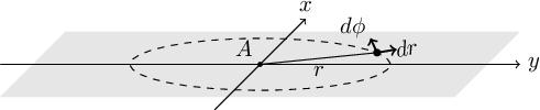
Figure 9.1: Two dimensional Cartesian and polar coordinates on a flat plane.
Assuming an object is placed at a certain position, which can be parameterized as \((x,y)\), or \((r,\phi)\), a general infinitesimal change in its position will place it in the coordinates \((x+dx,y+dy)\), or \((r+dr,\phi+d\phi)\). The distance (on the flat 2D surface) that is covered by this infinitesimal change in the static universe (\(ds_s\), the subscript signifies the static nature of this universe) can be written as:
$$ds_s^2=dx^2+dy^2=dr^2+r^2d\phi^2$$
The main question is this: how can the 2D creature incorporate the (possible) curvature in its universe when it’s calculating distances? The universe that it lives in might equally be a curved surface like Figure 9.2. The answer to this question but for a 3D being (us) is the whole purpose to this discussion. Here, we want to give the 2D creature (and later, ourselves) the tools to measure distances if the space (that hosts the objects) is curved.
Figure 9.2 assumes a spherical shell with radius \(R\) as the curved 2D plane for simplicity. The 2D plane is tangent to the spherical shell and only touches it at \(A\). This idea will be generalized later. The first step in measuring the distance in a curved space is to imagine a third dimension along the \(z\) axis as shown in Figure 9.2. For simplicity, the \(z\) axis is assumed to pass through the center of the spherical shell. Our imaginary 2D creature cannot visualize the third dimension or a curved 2D surface within it, so the remainder of this discussion is purely abstract for it (similar to us having difficulty in visualizing a 3D curved space in 4D). But since we are 3D creatures, we have the advantage of visualizing the following steps. Fortunately the 2D creature is already familiar with our mathematical constructs, so it can follow our reasoning.
With the third axis added, a generic infinitesimal change over the full 3D space corresponds to the distance:
$$ds_s^2=dx^2+dy^2+dz^2=dr^2+r^2d\phi^2+dz^2.$$
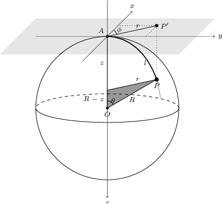
Figure 9.2: 2D spherical shell (centered on \(O\)) and flat plane (light gray) tangent to it at point \(A\).
It is very important to recognize that this change of distance is for any point in the 3D space, not just those changes that occur on the 2D spherical shell of Figure 9.2. Recall that our 2D friend can only do measurements on the 2D surfaces, not the full 3D space. So we have to constrain this general change to any change on the 2D spherical shell. To do that, let’s look at the arbitrary point \(P\) on the 2D spherical shell. Its image (\(P'\)) on the flat plain is also displayed. From the dark gray triangle, we see that
$$\sin\theta={r\over R},\quad\cos\theta={R-z\over R}.$$These relations allow the 2D creature to find the value of \(z\) (an abstract dimension for it) as a function of r (distance on a flat 2D plane, which it can visualize) and thus eliminate \(z\). From \(\sin^2\theta+\cos^2\theta=1\), we get \(z^2-2Rz+r^2=0\) and solving for \(z\), we find:
$$z=R\left(1\pm\sqrt{1-{r^2\over R^2}}\right).$$
The \(\pm\) can be understood from Figure 9.2: For each \(r\), there are two points on the sphere, one in the upper hemisphere and one in the lower hemisphere. An infinitesimal change in \(r\), will create the following infinitesimal change in \(z\):
$$dz={\mp r\over R}\left(1\over \sqrt{1-{r^2/R^2}}\right)dr.$$Using the positive signed equation instead of \(dz\) in the \(ds_s^2\) equation above, we get:
$$ds_s^2={dr^2\over 1-r^2/R^2}+r^2d\phi^2.$$
The derivation above was done for a spherical shell of radius \(R\) as a curved 2D surface. To generalize it to any surface, we can define \(K=1/R^2\) as the curvature parameter. Then the general infinitesimal change in a static universe can be written as:
$$ds_s^2={dr^2\over 1-Kr^2}+r^2d\phi^2.$$
Therefore, when \(K>0\) (and curvature is the same everywhere), we have a finite universe, where \(r\) cannot become larger than \(R\) as in Figure 9.2. When \(K=0\), we have a flat plane (Figure 9.1) and a negative \(K\) will correspond to an imaginary \(R\). The latter two cases may be infinite in area (which is not a simple concept, but mathematically can be modeled with \(r\) extending infinitely), or finite-area (like a cylinder is flat everywhere with \(ds_s^2={dx^2 + dy^2}\), but finite in one direction in size).
A very important issue that can be discussed now (while we are still in 2D and can actually visualize things) is that \(\overrightarrow{r}\) is tangent to the curved space at the observer’s position. In other words, it is on the gray flat surface of Figure 9.2, even when the universe if curved: \(\overrightarrow{r}=P'-A\). Therefore for the point \(P\) on a curved space, the raw coordinate \(r\) is the distance to \(P'\), not \(P\). The distance to the point \(P\) (at a specific coordinate \(r\) on the flat plane) over the curved surface (thick line in Figure 9.2) is called the proper distance and is displayed with \(l\). For the specific example of Figure 9.2, the proper distance can be calculated with: \(l=R\theta\) (\(\theta\) is in radians). Using the \(\sin\theta\) relation found above, we can find \(l\) as a function of \(r\):
$$\theta=\sin^{-1}\left({r\over R}\right)\quad\rightarrow\quad l(r)=R\sin^{-1}\left({r\over R}\right)$$
\(R\) is just an arbitrary constant and can be directly found from \(K\), so for cleaner equations, it is common practice to set \(R=1\), which gives: \(l(r)=\sin^{-1}r\). Also note that when \(R=1\), then \(l=\theta\). Generally, depending on the curvature, in a static universe the proper distance can be written as a function of the coordinate \(r\) as (from now on we are assuming \(R=1\)):
$$l(r)=\sin^{-1}(r)\quad(K>0),\quad\quad l(r)=r\quad(K=0),\quad\quad l(r)=\sinh^{-1}(r)\quad(K<0).$$With \(l\), the infinitesimal change of distance can be written in a more simpler and abstract form of
$$ds_s^2=dl^2+r^2d\phi^2.$$
Until now, we had assumed a static universe (not changing with time). But our observations so far appear to indicate that the universe is expanding (it is not static). Since there is no reason to expect the observed expansion is unique to our particular position of the universe, we expect the universe to be expanding at all points with the same rate at the same time. Therefore, to add a time dependence to our distance measurements, we can include a multiplicative scaling factor, which is a function of time: \(a(t)\). The functional form of \(a(t)\) comes from the cosmology, the physics we assume for it: general relativity, and the choice of whether the universe is uniform (‘homogeneous’) in density and curvature or inhomogeneous. In this section, the functional form of \(a(t)\) is irrelevant, so we can avoid these issues.
With this scaling factor, the proper distance will also depend on time. As the universe expands, the distance between two given points will shift to larger values. We thus define a distance measure, or coordinate, that is independent of time and thus does not ‘move’. We call it the comoving distance and display with \(\chi\) such that: \(l(r,t)=\chi(r)a(t)\). We have therefore, shifted the \(r\) dependence of the proper distance we derived above for a static universe to the comoving distance:
$$\chi(r)=\sin^{-1}(r)\quad(K>0),\quad\quad \chi(r)=r\quad(K=0),\quad\quad \chi(r)=\sinh^{-1}(r)\quad(K<0).$$
Therefore, \(\chi(r)\) is the proper distance to an object at a specific reference time: \(t=t_r\) (the \(r\) subscript signifies “reference”) when \(a(t_r)=1\). At any arbitrary moment (\(t\neq{t_r}\)) before or after \(t_r\), the proper distance to the object can be scaled with \(a(t)\).
Measuring the change of distance in a time-dependent (expanding) universe only makes sense if we can add up space and time243. But we can only add bits of space and time together if we measure them in the same units: with a conversion constant (similar to how 1000 is used to convert a kilometer into meters). Experimentally, we find strong support for the hypothesis that this conversion constant is the speed of light (or gravitational waves244) in a vacuum. This speed is postulated to be constant245 and is almost always written as \(c\). We can thus parameterize the change in distance on an expanding 2D surface as
$$ds^2=c^2dt^2-a^2(t)ds_s^2 = c^2dt^2-a^2(t)(d\chi^2+r^2d\phi^2).$$
9.1.2 Extending distance concepts to 3D 
The concepts of Distance on a 2D curved space are here extended to a 3D space that might be curved. We can start with the generic infinitesimal distance in a static 3D universe, but this time in spherical coordinates instead of polar coordinates. \(\theta\) is shown in Figure 9.2, but here we are 3D beings, positioned on \(O\) (the center of the sphere) and the point \(O\) is tangent to a 4D-sphere. In our 3D space, a generic infinitesimal displacement will correspond to the following distance in spherical coordinates:
$$ds_s^2=dx^2+dy^2+dz^2=dr^2+r^2(d\theta^2+\sin^2{\theta}d\phi^2).$$
Like the 2D creature before, we now have to assume an abstract dimension which we cannot visualize easily. Let’s call the fourth dimension \(w\), then the general change in coordinates in the full four dimensional space will be:
$$ds_s^2=dr^2+r^2(d\theta^2+\sin^2{\theta}d\phi^2)+dw^2.$$
But we can only work on a 3D curved space, so following exactly the same steps and conventions as our 2D friend, we arrive at:
$$ds_s^2={dr^2\over 1-Kr^2}+r^2(d\theta^2+\sin^2{\theta}d\phi^2).$$
In a non-static universe (with a scale factor a(t)), the distance can be written as:
$$ds^2=c^2dt^2-a^2(t)[d\chi^2+r^2(d\theta^2+\sin^2{\theta}d\phi^2)].$$
9.1.3 Invoking CosmicCalculator 
CosmicCalculator will calculate cosmological variables based on the input parameters. The executable name is astcosmiccal with the following general template
$ astcosmiccal [OPTION...] ...
One line examples:
## Print basic cosmological properties at redshift 2.5: $ astcosmiccal -z2.5 ## Only print Comoving volume over 4pi stradian to z (Mpc^3): $ astcosmiccal --redshift=0.8 --volume ## Print redshift and age of universe when Lyman-alpha line is ## at 6000 angstrom (another way to specify redshift). $ astcosmiccal --obsline=Ly-alpha,6000 --age ## Print luminosity distance, angular diameter distance and age ## of universe in one row at redshift 0.4 $ astcosmiccal -z0.4 -LAg ## Assume Lambda and matter density of 0.7 and 0.3 and print ## basic cosmological parameters for redshift 2.1: $ astcosmiccal -l0.7 -m0.3 -z2.1 ## Print wavelength of all pre-defined spectral lines when ## Lyman-alpha is observed at 4000 Angstroms. $ astcosmiccal --obsline=Ly-alpha,4000 --listlinesatz
The input parameters (current matter density, etc.) can be given as command-line options or in the configuration files, see Configuration files. For a definition of the different parameters, please see the sections prior to this. If no redshift is given, CosmicCalculator will just print its input parameters and abort. For a full list of the input options, please see CosmicCalculator input options.
Without any particular output requested (and only a given redshift), CosmicCalculator will print all basic cosmological calculations (one per line) with some explanations before each. This can be good when you want a general feeling of the conditions at a specific redshift. Alternatively, if any specific calculation(s) are requested (its possible to call more than one), only the requested value(s) will be calculated and printed with one character space between them. In this case, no description or units will be printed. See CosmicCalculator basic cosmology calculations for the full list of these options along with some explanations how when/how they can be useful.
Another common operation in observational cosmology is dealing with spectral lines at different redshifts. CosmicCalculator also has features to help in such situations, please see CosmicCalculator spectral line calculations.
- CosmicCalculator input options
- CosmicCalculator basic cosmology calculations
- CosmicCalculator spectral line calculations
9.1.3.1 CosmicCalculator input options 
The inputs to CosmicCalculator can be specified with the following options:
- -z FLT
- --redshift=FLT
The redshift of interest. There are two other ways that you can specify the target redshift: 1) Spectral lines and their observed wavelengths, see --obsline. 2) Velocity, see --velocity. Hence this option cannot be called with --obsline or --velocity.
- -y FLT
- --velocity=FLT
Input velocity in km/s. The given value will be converted to redshift internally, and used in any subsequent calculation. This option is thus an alternative to
--redshiftor--obsline, it cannot be used with them. The conversion will be done with the more general and accurate relativistic equation of \(1+z=\sqrt{(c+v)/(c-v)}\), not the simplified \(z\approx v/c\).- -H FLT
- --H0=FLT
Current expansion rate (in km sec\(^{-1}\) Mpc\(^{-1}\)).
- -l FLT
- --olambda=FLT
Cosmological constant density divided by the critical density in the current Universe (\(\Omega_{\Lambda,0}\)).
- -m FLT
- --omatter=FLT
Matter (including massive neutrinos) density divided by the critical density in the current Universe (\(\Omega_{m,0}\)).
- -r FLT
- --oradiation=FLT
Radiation density divided by the critical density in the current Universe (\(\Omega_{r,0}\)).
- -O STR/FLT,FLT 
- --obsline=STR/FLT,FLT
Find the redshift to use in next steps based on the rest-frame and observed wavelengths of a line. This option is thus an alternative to
--redshiftor--velocity, it cannot be used with them.The first argument identifies the line. It can be one of the standard names, or any rest-frame wavelength in Angstroms. The second argument is the observed wavelength of that line. For example, --obsline=Ly-alpha,6000 is the same as --obsline=1215.64,6000. Wavelengths are assumed to be in Angstroms by default (other units can be selected with --lineunit, see CosmicCalculator spectral line calculations).
The list of pre-defined names for the lines in Gnuastro’s database is available by running
$ astcosmiccal --listlines
9.1.3.2 CosmicCalculator basic cosmology calculations 
By default, when no specific calculations are requested, CosmicCalculator will print a complete set of all its calculators (one line for each calculation, see Invoking CosmicCalculator). The full list of calculations can be useful when you do not want any specific value, but just a general view. In other contexts (for example, in a batch script or during a discussion), you know exactly what you want and do not want to be distracted by all the extra information.
You can use any number of the options described below in any order. When any of these options are requested, CosmicCalculator’s output will just be a single line with a single space between the (possibly) multiple values. In the example below, only the tangential distance along one arc-second (in kpc), absolute magnitude conversion, and age of the universe at redshift 2 are printed (recall that you can merge short options together, see Options).
$ astcosmiccal -z2 -sag 8.585046 44.819248 3.289979
Here is one example of using this feature in scripts: by adding the following two lines in a script to keep/use the comoving volume with varying redshifts:
z=3.12 vol=$(astcosmiccal --redshift=$z --volume)
In a script, this operation might be necessary for a large number of objects (several of galaxies in a catalog for example). So the fact that all the other default calculations are ignored will also help you get to your result faster.
If you are indeed dealing with many (for example, thousands) of redshifts, using CosmicCalculator is not the best/fastest solution. Because it has to go through all the configuration files and preparations for each invocation. To get the best efficiency (least overhead), we recommend using Gnuastro’s cosmology library (see Cosmology library (cosmology.h)). CosmicCalculator also calls the library functions defined there for its calculations, so you get the same result with no overhead. Gnuastro also has libraries for easily reading tables into a C program, see Table input output (table.h). Afterwards, you can easily build and run your C program for the particular processing with BuildProgram.
If you just want to inspect the value of a variable visually, the description (which comes with units) might be more useful. In such cases, the following command might be better. The other calculations will also be done, but they are so fast that you will not notice on modern computers (the time it takes your eye to focus on the result is usually longer than the processing: a fraction of a second).
$ astcosmiccal --redshift=0.832 | grep volume
The full list of CosmicCalculator’s specific calculations is present below in two groups: basic cosmology calculations and those related to spectral lines. In case you have forgot the units, you can use the --help option which has the units along with a short description.
- -e
- --usedredshift
The redshift that was used in this run. In many cases this is the main input parameter to CosmicCalculator, but it is useful in others. For example, in combination with --obsline (where you give an observed and rest-frame wavelength and would like to know the redshift) or with --velocity (where you specify the velocity instead of redshift). Another example is when you run CosmicCalculator in a loop, while changing the redshift and you want to keep the redshift value with the resulting calculation.
- -Y
- --usedvelocity
The velocity (in km/s) that was used in this run. The conversion from redshift will be done with the more general and accurate relativistic equation of \(1+z=\sqrt{(c+v)/(c-v)}\), not the simplified \(z\approx v/c\).
- -G
- --agenow
The current age of the universe (given the input parameters) in Ga (Giga annum, or billion years).
- -C
- --criticaldensitynow
The current critical density (given the input parameters) in grams per cubic centimeter (\(g/cm^3\)).
- -d
- --properdistance
The proper distance (at the current time, i.e. in comoving units) to an object at the given redshift in Megaparsecs (Mpc). See Distance on a 2D curved space for a description of the proper distance.
- -A
- --angulardiamdist
The angular diameter distance to an object at a given redshift in Megaparsecs (Mpc).
- -s
- --arcsectandist
The tangential distance covered by 1 arc-second at a given redshift in physical (not comoving) kilo-parsecs (kpc). This can be useful when trying to estimate the resolution or pixel scale of an instrument (usually in units of arc-seconds) required for a galaxy of a given physical size at a given redshift.
For an arc subtending one degree at a high redshift \(z\), multiplying the result by 3600 will, of course, give the (tangential) length of an arc subtending one degree, but it will still be in physical units. However, at one degree, the comoving separation for redshifts from 1 to 10 is about 100 Mpc give or take 50% or so for nearly \(\Lambda{}\)CDM models. In other words, this is the cosmic web scale, where comoving units usually make more sense than physical units, e.g. for large-scale structure correlation functions or the baryon acoustic oscillation scale. If comoving units are appropriate, as will typically be the case for the degree scale, you must also multiply by \((1+z)\).
- -L
- --luminositydist
The luminosity distance to object at given redshift in Megaparsecs (Mpc).
- -u 
- --distancemodulus
The bolometric (across the full electromagnetic spectrum) distance modulus (\(DM\)) at the given redshift assuming no intermediate absorption. The distance modulus allows the conversion of observed (\(m\), distance dependent) to absolute (\(M\), independent of distance; or the same distance of 10 parsecs for all objects) magnitudes. In other words, \(DM=m-M\), or \(M=m-DM\). From the absolute magnitude, we can derive the luminosity of the source; see
mag-to-luminosityin Unit conversion operators.The two conditions above are very important to remember when using this option:
- In practice we do not observe the bolometric magnitude of an object: any instrument’s hardware is limited to a certain wavelength range and incoming photons outside that range will not be measured.
Therefore, as regards the filter and spectrum, the distance modulus can be used in the following two cases:
- At smaller distances (where the filter on the observed spectrum covers approximately the same region on the rest frame spectrum).
- The observed bolometric magnitude of the source has been calculated (based on model-fitting, or combining data from many surveys to cover the whole electromagnetic spectrum) and is being used as input
At higher distances, it is important to account for “K-correction” because the filter’s rest frame coverage over the rest frame spectrum of the source will decrease (compared to the filter’s observed coverage in the source’s observed spectrum). For details see Hogg et al. 2002 and Blanton and Roweis 2007. A simplified correction (assuming a flat SED) to the distance modulus is available in the --absmagconv option below.
- Intermediate absorption (from the source to your telescope) can happen in multiple stages. For example, the Earth is located inside the Milky Way which has an interstellar medium (ISM) that will absorb some of the flux coming from extra-galactic sources behind them. After measuring the magnitude of your source, it is therefore important to find the Milky Way extinction in the direction of your source and add it to your source’s flux. Inside Gnuastro, the Query program gives you direct access to the NED Extinction Calculator as described in Available databases.
- In practice we do not observe the bolometric magnitude of an object: any instrument’s hardware is limited to a certain wavelength range and incoming photons outside that range will not be measured.
Therefore, as regards the filter and spectrum, the distance modulus can be used in the following two cases:
- -a
- --absmagconv
Corrected distance modulus: accounting for the thinner width of the filter at higher redshift by subtracting \(2.5\log{(1+z)}\) from the distance modulus (assuming a flat SED for the galaxy). However, no astronomical object has a flat SED across all wavelengths, so this should be taken as a zero-th order K-correction: just a crude statistical approximate that may under/over-estimate the actual value badly in special cases (for example when the omitted region has/misses a strong spectral feature). See the description of --distancemodulus for more.
- -g
- --age
Age of the universe at given redshift in Ga (Giga-annum, or billion years).
- -b
- --lookbacktime
The look-back time to a given redshift in Ga (Giga annum, or billion years). The look-back time at a given redshift is defined as the current age of the universe (--agenow) minus the age of the universe at the given redshift.
- -c
- --criticaldensity
The critical density at given redshift in grams per centimeter-cube (\(g/cm^3\)).
- -v
- --onlyvolume
The comoving volume in cubic Megaparsecs (Mpc\(^3\)) through to the desired redshift, based on the input parameters.
9.1.3.3 CosmicCalculator spectral line calculations 
At different redshifts, observed spectral lines are shifted compared to their rest frame wavelengths with this simple relation: \(\lambda_{obs}=\lambda_{rest}(1+z)\). Although this relation is very simple and can be done for one line in the head (or a simple calculator!), it slowly becomes tiring when dealing with a lot of lines or redshifts, or some precision is necessary. The options in this section are thus provided to greatly simplify usage of this simple equation, and also helping by storing a list of pre-defined spectral line wavelengths.
For example, if you want to know the wavelength of the \(H\alpha\) line (at 6562.8 Angstroms in rest frame), when \(Ly\alpha\) is at 8000 Angstroms, you can call CosmicCalculator like the first example below. And if you want the wavelength of all pre-defined spectral lines at this redshift, you can use the second command.
$ astcosmiccal --obsline=lyalpha,8000 --lineatz=halpha $ astcosmiccal --obsline=lyalpha,8000 --listlinesatz
Bellow you can see the printed/output calculations of CosmicCalculator that are related to spectral lines. Note that --obsline is an input parameter, so it is discussed (with the full list of known lines) in CosmicCalculator input options.
- --listlines
List the pre-defined rest frame spectral line wavelengths and their names on standard output, then abort CosmicCalculator. The units of the displayed wavelengths for each line can be determined with --lineunit (see below).
When this option is given, other operations on the command-line will be ignored. This is convenient when you forget the specific name of the spectral line used within Gnuastro, or when you forget the exact wavelength of a certain line.
These names can be used with the options that deal with spectral lines, for example, --obsline and --lineatz (CosmicCalculator basic cosmology calculations).
The format of the output list is a two-column table, with Gnuastro’s text table format (see Gnuastro text table format). Therefore, if you are only looking for lines in a specific range, you can pipe the output into Gnuastro’s table program and use its --range option on the
wavelength(first) column. For example, if you only want to see the lines between 4000 and 6000 Angstroms, you can run this command:$ astcosmiccal --listlines \ | asttable --range=wavelength,4000,6000And if you want to use the list later and have it as a table in a file, you can easily add the --output (or -o) option to the
asttablecommand, and specify the filename, for example, --output=lines.fits or --output=lines.txt.- --listlinesatz
Similar to --listlines (above), but the printed wavelength is not in the rest frame, but redshifted to the given redshift. Recall that the redshift can be specified by --redshift directly or by --obsline, see CosmicCalculator input options. For an example usage of this option, see Viewing spectra and redshifted lines.
- -i STR/FLT
- --lineatz=STR/FLT
The wavelength of the specified line at the redshift given to CosmicCalculator. The line can be specified either by its name or directly as a number (its wavelength). The units of the displayed wavelengths for each line can be determined with --lineunit (see below).
To get the list of pre-defined names for the lines and their wavelength, you can use the --listlines option, see CosmicCalculator input options. In the former case (when a name is given), the returned number is in units of Angstroms. In the latter (when a number is given), the returned value is the same units of the input number (assuming it is a wavelength).
- --lineunit=STR
The units to display line wavelengths above. It can take the following four values. If you need any other unit, please contact us at
bug-gnuastro@gnu.org.mMeter.
micro-mMicrometer or \(10^{-6}m\).
nano-mNanometer, or \(10^{-9}m\).
angstromAngstrom or \(10^{-10}m\); the default unit when this option is not called.
10 Installed scripts 
Gnuastro’s programs (introduced in previous chapters) are designed to be highly modular and thus contain lower-level operations on the data.
However, in many contexts, certain higher-level are also shared between many contexts.
For example, a sequence of calls to multiple Gnuastro programs, or a special way of running a program and treating the output.
To facilitate such higher-level data analysis, Gnuastro also installs some scripts on your system with the (astscript-) prefix (in contrast to the other programs that only have the ast prefix).
Like all of Gnuastro’s source code, these scripts are also heavily commented.
They are written in portable shell scripts (command-line environments), which does not need compilation.
Therefore, if you open the installed scripts in a text editor, you can actually read them246.
For example, with this command (just replace nano with your favorite text editor, like emacs or vim):
$ nano $(which astscript-NAME)
Shell scripting is the same language that you use when typing on the command-line. Therefore shell scripting is much more widely known and used compared to C (the language of other Gnuastro programs). Because Gnuastro’s installed scripts do higher-level operations, customizing these scripts for a special project will be more common than the programs.
These scripts also accept options and are in many ways similar to the programs (see Common options) with some minor differences:
- Currently they do not accept configuration files themselves.
However, the configuration files of the Gnuastro programs they call are indeed parsed and used by those programs.
As a result, they do not have the following options: --checkconfig, --config, --lastconfig, --onlyversion, --printparams, --setdirconf and --setusrconf.
- They do not directly allocate any memory, so there is no --minmapsize.
- They do not have an independent --usage option: when called with --usage, they just recommend running --help.
- The output of --help is not configurable like the programs (see --help).
- The scripts will commonly use your installed shell and other basic command-line tools (for example, AWK or SED). Different systems have different versions and implementations of these basic tools (for example, GNU/Linux systems use GNU Bash, GNU AWK and GNU SED which are far more advanced and up to date then the minimalist AWK and SED of most other systems). Therefore, unexpected errors in these tools might come up when you run these scripts on non-GNU/Linux operating systems. If you do confront such strange errors, please submit a bug report so we fix it as soon as possible (see Report a bug).
- Sort FITS files by night
- Generate radial profile
- SAO DS9 region files from table
- Viewing FITS file contents with DS9 or TOPCAT
- Zero point estimation
- Pointing pattern simulation
- Color images with gray faint regions
- PSF construction and subtraction
10.1 Sort FITS files by night 
FITS images usually contain (several) keywords for preserving important dates.
In particular, for lower-level data, this is usually the observation date and time (for example, stored in the DATE-OBS keyword value).
When analyzing observed datasets, many calibration steps (like the dark, bias or flat-field), are commonly calculated on a per-observing-night basis.
However, the FITS standard’s date format (YYYY-MM-DDThh:mm:ss.ddd) is based on the western (Gregorian) calendar.
Dates that are stored in this format are complicated for automatic processing: a night starts in the final hours of one calendar day, and extends to the early hours of the next calendar day.
As a result, to identify datasets from one night, we commonly need to search for two dates.
However calendar peculiarities can make this identification very difficult.
For example, when an observation is done on the night separating two months (like the night starting on March 31st and going into April 1st), or two years (like the night starting on December 31st 2018 and going into January 1st, 2019).
To account for such situations, it is necessary to keep track of how many days are in a month, and leap years, etc.
Gnuastro’s astscript-sort-by-night script is created to help in such important scenarios. It uses Fits to convert the FITS date format into the Unix epoch time (number of seconds since 00:00:00 of January 1st, 1970), using the --datetosec option. The Unix epoch time is a single number (integer, if not given in sub-second precision), enabling easy comparison and sorting of dates after January 1st, 1970.
You can use this script as a basis for making a much more highly customized sorting script. Here are some examples
- If you need to copy the files, but only need a single extension (not the whole file), you can add a step just before the making of the symbolic links, or copies, and change it to only copy a certain extension of the FITS file using the Fits program’s --copy option, see HDU information and manipulation.
- If you need to classify the files with finer detail (for example, the purpose of the dataset), you can add a step just before the making of the symbolic links, or copies, to specify a file-name prefix based on other certain keyword values in the files.
For example, when the FITS files have a keyword to specify if the dataset is a science, bias, or flat-field image.
You can read it and to add a
sci-,bias-, orflat-to the created file (after the --prefix) automatically.For example, let’s assume the observing mode is stored in the hypothetical
MODEkeyword, which can have three values ofBIAS-IMAGE,SCIENCE-IMAGEandFLAT-EXP. With the step below, you can generate a mode-prefix, and add it to the generated link/copy names (just correct the filename and extension of the first line to the script’s variables):modepref=$(astfits infile.fits -h1 \ | sed -e"s/'/ /g" \ | awk '$1=="MODE"{ \ if($3=="BIAS-IMAGE") print "bias-"; \ else if($3=="SCIENCE-IMAGE") print "sci-"; \ else if($3==FLAT-EXP) print "flat-"; \ else print $3, "NOT recognized"; exit 1}')Here is a description of it. We first use
astfitsto print all the keywords in extension1of infile.fits. In the FITS standard, string values (that we are assuming here) are placed in single quotes (') which are annoying in this context/use-case. Therefore, we pipe the output ofastfitsintosedto remove all such quotes (substituting them with a blank space). The result is then piped to AWK for giving us the final mode-prefix: with$1=="MODE", we ask AWK to only consider the line where the first column isMODE. There is an equal sign between the key name and value, so the value is the third column ($3in AWK). We thus use a simpleif-elsestructure to look into this value and print our custom prefix based on it. The output of AWK is then stored in themodeprefshell variable which you can add to the link/copy name.With the solution above, the increment of the file counter for each night will be independent of the mode. If you want the counter to be mode-dependent, you can add a different counter for each mode and use that counter instead of the generic counter for each night (based on the value of
modepref). But we will leave the implementation of this step to you as an exercise.
10.1.1 Invoking astscript-sort-by-night 
This installed script will read a FITS date formatted value from the given keyword, and classify the input FITS files into individual nights. For more on installed scripts please see (see Installed scripts). This script can be used with the following general template:
$ astscript-sort-by-night [OPTION...] FITS-files
One line examples:
## Use the DATE-OBS keyword $ astscript-sort-by-night --key=DATE-OBS /path/to/data/*.fits ## Make links to the input files with the `img-' prefix $ astscript-sort-by-night --link --prefix=img- /path/to/data/*.fits
This script will look into a HDU/extension (--hdu) for a keyword (--key) in the given FITS files and interpret the value as a date. The inputs will be separated by "night"s (11:00a.m to next day’s 10:59:59a.m, spanning two calendar days, exact hour can be set with --hour).
The default output is a list of all the input files along with the following two columns: night number and file number in that night (sorted by time). With --link a symbolic link will be made (one for each input) that contains the night number, and number of file in that night (sorted by time), see the description of --link for more. When --copy is used instead of a link, a copy of the inputs will be made instead of symbolic link.
Below you can see one example where all the target-*.fits files in the data directory should be separated by observing night according to the DATE-OBS keyword value in their second extension (number 1, recall that HDU counting starts from 0).
You can see the output after the ls command.
$ astscript-sort-by-night -pimg- -h1 -kDATE-OBS data/target-*.fits $ ls img-n1-1.fits img-n1-2.fits img-n2-1.fits ...
The outputs can be placed in a different (already existing) directory by including that directory’s name in the --prefix value, for example, --prefix=sorted/img- will put them all under the sorted directory.
This script can be configured like all Gnuastro’s programs (through command-line options, see Common options), with some minor differences that are described in Installed scripts. The particular options to this script are listed below:
- -h STR
- --hdu=STR
The HDU/extension to use in all the given FITS files. All of the given FITS files must have this extension.
- -k STR
- --key=STR
The keyword name that contains the FITS date format to classify/sort by.
- -H FLT
- --hour=FLT
The hour that defines the next “night”. By default, all times before 11:00a.m are considered to belong to the previous calendar night. If a sub-hour value is necessary, it should be given in units of hours, for example, --hour=9.5 corresponds to 9:30a.m.
- -l
- --link
Create a symbolic link for each input FITS file. This option cannot be used with --copy. The link will have a standard name in the following format (variable parts are written in
CAPITALletters and described after it):PnN-I.fits
PThis is the value given to --prefix. By default, its value is
./(to store the links in the directory this script was run in). See the description of--prefixfor more.NThis is the night-counter: starting from 1.
Nis just incremented by 1 for the next night, no matter how many nights (without any dataset) there are between two subsequent observing nights (its just an identifier for each night which you can easily map to different calendar nights).IFile counter in that night, sorted by time.
- -c
- --copy
Make a copy of each input FITS file with the standard naming convention described in --link. With this option, instead of making a link, a copy is made. This option cannot be used with --link.
- -p STR
- --prefix=STR
Prefix to append before the night-identifier of each newly created link or copy. This option is thus only relevant with the --copy or --link options. See the description of --link for how it is used. For example, with --prefix=img-, all the created file names in the current directory will start with
img-, making outputs like img-n1-1.fits or img-n3-42.fits.--prefix can also be used to store the links/copies in another directory relative to the directory this script is being run (it must already exist). For example,
--prefix=/path/to/processing/img-will put all the links/copies in the /path/to/processing directory, and the files (in that directory) will all start with img-.- --stdintimeout=INT
Number of micro-seconds to wait for standard input within this script. This does not correspond to general inputs into the script, inputs to the script should always be given as a file. However, within the script, pipes are often used to pass the output of one program to another. The value given to this option will be passed to those internal pipes. When running this script, if you confront an error, saying “No input!”, you should be able to fix it by giving a larger number to this option (the default value is 10000000 micro-seconds or 10 seconds).
10.2 Generate radial profile 
The 1 dimensional radial profile of an object is an important parameter in many aspects of astronomical image processing. For example, you want to study how the light of a galaxy is distributed as a function of the radial distance from the center. In other cases, the radial profile of a star can show the PSF (see Point spread function). Gnuastro’s astscript-radial-profile script is created to obtain such radial profiles for one object within an image. This script uses MakeProfiles to generate elliptical apertures with the values equal to the distance from the center of the object and MakeCatalog for measuring the values over the apertures.
10.2.1 Invoking astscript-radial-profile 
This installed script will measure the radial profile of an object within an image. A general overview of this script has been published in Infante-Sainz et al. 2024); please cite it if this script proves useful in your research. For more on installed scripts please see (see Installed scripts). This script can be used with the following general template:
$ astscript-radial-profile [OPTION...] FITS-file
Examples:
## Generate the radial profile with default options (assuming the
## object is in the center of the image, and using the mean).
$ astscript-radial-profile image.fits
## Generate the radial profile centered at x=44 and y=37 (in pixels),
## up to a radial distance of 19 pixels, use the mean value.
$ astscript-radial-profile image.fits --center=44,37 --rmax=19
## Generate a 2D polar plot with the same properties as above:
$ astscript-radial-profile image.fits --center=44,37 --rmax=19 \
--polar
## Generate the radial profile centered at x=44 and y=37 (in pixels),
## up to a radial distance of 100 pixels, compute sigma clipped
## mean and standard deviation (sigclip-mean and sigclip-std) using
## 5 sigma and 0.1 tolerance (default is 3 sigma and 0.2 tolerance).
$ astscript-radial-profile image.fits --center=44,37 --rmax=100 \
--sigmaclip=5,0.1 \
--measure=sigclip-mean,sigclip-std
## Generate the radial profile centered at RA=20.53751695,
## DEC=0.9454292263, up to a radial distance of 88 pixels,
## axis ratio equal to 0.32, and position angle of 148 deg.
## Name the output table as `radial-profile.fits'
$ astscript-radial-profile image.fits --mode=wcs \
--center=20.53751695,0.9454292263 \
--rmax=88 --axis-ratio=0.32 \
--position-angle=148 -oradial-profile.fits
## Generate the radial profile centered at RA=40.062675270971,
## DEC=-8.1511992735126, up to a radial distance of 20 pixels,
## and calculate the SNR using the INPUT-NO-SKY and SKY-STD
## extensions of the NoiseChisel output file.
$ astscript-radial-profile image_detected.fits -hINPUT-NO-SKY \
--mode=wcs --measure=sn \
--center=40.062675270971,-8.1511992735126 \
--rmax=20 --stdhdu=SKY_STD
## Generate the radial profile centered at RA=40.062675270971,
## DEC=-8.1511992735126, up to a radial distance of 20 pixels,
## and compute the SNR with a fixed value for std, std=10.
$ astscript-radial-profile image.fits -h1 --mode=wcs --rmax=20 \
--center=40.062675270971,-8.1511992735126 \
--measure=sn --instd=10
## Generate the radial profile centered at X=1201, Y=1201 pixels, up
## to a radial distance of 20 pixels and compute the median and the
## SNR using the first extension of sky-std.fits as the dataset for std
## values.
$ astscript-radial-profile image.fits -h1 --mode=img --rmax=20 \
--center=1201,1201 --measure=median,sn \
--instd=sky-std.fits
This installed script will read a FITS image and will use it as the basis for constructing the radial profile. The output radial profile is a table (FITS or plain-text) containing the radial distance from the center in the first row and the specified measurements in the other columns (mean, median, sigclip-mean, sigclip-median, etc.).
To measure the radial profile, this script needs to generate temporary files. All these temporary files will be created within the directory given to the --tmpdir option. When --tmpdir is not called, a temporary directory (with a name based on the inputs) will be created in the running directory. If the directory does not exist at run-time, this script will create it. After the output is created, this script will delete the directory by default, unless you call the --keeptmp option.
With the default options, the script will generate a circular radial profile using the mean value and centered at the center of the image. In order to have more flexibility, several options are available to configure for the desired radial profile. In this sense, you can change the center position, the maximum radius, the axis ratio and the position angle (elliptical apertures are considered), the operator for obtaining the profiles, and others (described below).
|
Debug your profile: to debug your results, especially close to the center of your object, you can see the radial distance associated to every pixel in your input. To do this, use --keeptmp to keep the temporary files, and compare crop.fits (crop of your input image centered on your desired coordinate) with apertures.fits (radial distance of each pixel). |
|
Finding properties of your elliptical target: you want to measure the radial profile of a galaxy, but do not know its exact location, position angle or axis ratio. To obtain these values, you can use NoiseChisel to detect signal in the image, feed it to Segment to do basic segmentation, then use MakeCatalog to measure the center (--x and --y in MakeCatalog), axis ratio (--axis-ratio) and position angle (--position-angle). |
|
Masking other sources: The image of an astronomical object will usually have many other sources with your main target.
A crude solution is to use sigma-clipped measurements for the profile.
However, sigma-clipped measurements can easily be biased when the number of sources at each radial distance increases at larger distances.
Therefore a robust solution is to mask all other detections within the image.
You can use NoiseChisel and Segment to detect and segment the sources, then set all pixels that do not belong to your target to blank using Arithmetic (in particular, its |
- -h STR
- --hdu=STR
The HDU/extension of the input image to use.
- -o STR
- --output=STR
Filename of measured radial profile. It can be either a FITS table, or plain-text table (determined from your given file name suffix).
- -c FLT[,FLT[,...]]
- --center=FLT[,FLT[,...]]
The central position of the radial profile. This option is used for placing the center of the profiles. This parameter is used in Crop to center and crop the region. The positions along each dimension must be separated by a comma (,) and fractions are also acceptable. The number of values given to this option must be the same as the dimensions of the input dataset. The units of the coordinates are read based on the value to the --mode option, see below.
- -O STR
- --mode=STR
Interpret the center position of the object (values given to --center) in image or WCS coordinates. This option thus accepts only two values: img or wcs. By default, it is --mode=img.
- -R FLT
- --rmax=FLT
Maximum radius for the radial profile (in pixels). By default, the radial profile will be computed up to a radial distance equal to the maximum radius that fits into the image (assuming circular shape).
- -P INT
- --precision=INT
The precision (number of digits after the decimal point) in resolving the radius. The default value is --precision=0 (or -P0), and the value cannot be larger than 6. A higher precision is primarily useful when the very central few pixels are important for you. A larger precision will over-resolve larger radial regions, causing scatter to significantly affect the measurements.
For example, in the command below, we will generate the radial profile of an imaginary source (at RA,DEC of 1.23,4.567) and check the output without setting a precision:
$ astscript-radial-profile image.fits --center=1.23,4.567 \ --mode=wcs --measure=mean,area --rmax=10 \ --output=radial.fits --quiet $ asttable radial.fits --head=10 -ffixed -p4 0.0000 0.0139 1 1.0000 0.0048 8 2.0000 0.0023 16 3.0000 0.0015 20 4.0000 0.0011 24 5.0000 0.0008 40 6.0000 0.0006 36 7.0000 0.0005 48 8.0000 0.0004 56 9.0000 0.0003 56Let’s repeat the command above, but use a precision of 3 to resolve more finer details of the radial profile, while only printing the top 10 rows of the profile:
$ astscript-radial-profile image.fits --center=1.23,4.567 \ --mode=wcs --measure=mean,area --rmax=10 \ --precision=3 --output=radial.fits --quiet $ asttable radial.fits --head=10 -ffixed -p4 0.0000 0.0139 1 1.0000 0.0056 4 1.4140 0.0040 4 2.0000 0.0027 4 2.2360 0.0024 8 2.8280 0.0018 4 3.0000 0.0017 4 3.1620 0.0016 8 3.6050 0.0013 8 4.0000 0.0011 4Do you see how many more radii have been added? Between 1.0 and 2.0, we now have one extra radius, between 2.0 to 3.0, we have two new radii and so on. If you go to larger and larger radii, you will notice that they get resolved into many sub-components and the number of pixels used in each measurement will not be significant (you can already see that in the comparison above). This has two problems: 1. statistically, the scatter in larger radii (where the signal-to-noise ratio is usually low will make it hard to interpret the profile. 2. technically, the output table will have many more rows!
Use higher precision only for small radii: If you want to look at the whole profile (or the outer parts!), don’t set the precision, the default mode is usually more than enough! But when you are targeting the very central few pixels (usually less than a pixel radius of 5), use a higher precision.
- -v INT
- --oversample=INT
Oversample the input dataset to the fraction given to this option. Therefore if you set --rmax=20 for example, and --oversample=5, your output will have 100 rows (without --oversample it will only have 20 rows). Unless the object is heavily undersampled (the pixels are larger than the actual object), this method provides a much more accurate result and there are sufficient number of pixels to get the profile accurately.
Due to the discrete nature of pixels, if you use this option to oversample your profile, set --precision=0. Otherwise, your profile will become step-like (with several radii having a single value).
- -u INT
- --undersample=INT
Undersample the input dataset by the number given to this option. This option is for considering larger apertures than the original pixel size (aperture size is equal to 1 pixel). For example, if a radial profile computed by default has 100 different radii (apertures of 1 pixel width), by considering --undersample=2 the radial profile will be computed over apertures of 2 pixels, so the final radial profile will have 50 different radii. This option is good to measure over a larger number of pixels to improve the measurement.
- -Q FLT
- --axis-ratio=FLT
The axis ratio of the apertures (minor axis divided by the major axis in a 2D ellipse). By default (when this option is not given), the radial profile will be circular (axis ratio of 1). This parameter is used as the option --qcol in the generation of the apertures with
astmkprof.- -p FLT
- --position-angle=FLT
The position angle (in degrees) of the profiles relative to the first FITS axis (horizontal when viewed in SAO DS9). By default, it is --position-angle=0, which means that the semi-major axis of the profiles will be parallel to the first FITS axis.
- -a FLT,FLT 
- --azimuth=FLT,FLT
Limit the profile to the given azimuthal angle range (in degrees, from 0 to 360) from the major axis (defined by --position-angle) of each call to this option. The radial profile will therefore be created on a wedge-like shape, not the full circle/ellipse. The pixel containing the center of the profile will always be included in the profile (because it contains all azimuthal angles!).
If the first angle is smaller than the second (for example, --azimuth=10,80), the region between, or inside, the two angles will be used. Otherwise (for example, --azimuth=80,10), the region outside the two angles will be used. The latter case can be useful when you want to ignore part of the 2D shape (for example, due to a bright star that can be contaminating it).
This option can be called more than once; for example, --azimuth=80,100 --azimuth=260,280. In such cases, all given azimuthal ranges will be used. In the example above, two wedge-like shapes will be used to construct the profile: between angles of 80 to 100 degrees, and between 260 and 280 degrees.
You can see the shape of the region used by adding the --keeptmp option. Afterwards, you can view the values.fits and apertures.fits files of the temporary directory with a FITS image viewer like SAO DS9. You can use Viewing FITS file contents with DS9 or TOPCAT to open them together in one instance of DS9, with both frames matched and locked (for easy comparison in case you want to zoom-in or out). For example, see the commands below (based on your target object, just change the image name, center, position angle, etc.):
## Generate the radial profile $ astscript-radial-profile image.fits --center=1.234,6.789 \ --mode=wcs --rmax=50 --position-angle=20 \ --axis-ratio=0.8 --azimuth=95,150 --keeptmp \ --tmpdir=radial-tmp ## Visually check the values and apertures used. $ astscript-fits-view radial-tmp/values.fits \ radial-tmp/apertures.fits- -g
- --polar
Generate a 2D polar-plot image in the second HDU of the output (called
POLAR-PLOT). A polar plot is a projection of the original pixel grid into polar coordinates (where the horizontal axis is the azimuthal angle and the vertical axis is the radius).By default it assumes the full azimuthal range (from 0 to 360 degrees); if a narrower azimuthal range is desired, use --azimuth (for example --azimuth=30,50 to only generate the polar plot between 30 and 50 degrees of azimuth).
The output image contains WCS information to map the pixel coordinates into the polar coordinates. This is especially useful when the azimuthal range is not the full range: the first pixel in the horizontal axis is not 0 degrees.
Currently, the polar plot cannot to be used with --oversample and --undersample options (please get in touch with us if you need it). Until it is implemented, you can use the --scale option of Warp to do the oversampling of the input image yourself and generate the polar plot from that. A comprehensive overview of this option has been published in Eskandarlou et al. 2024. If this script yields useful results in your research, please be sure to cite it.
- -m STR
- --measure=STR
The operator for measuring the values over each radial distance. The values given to this option will be directly passed to MakeCatalog. As a consequence, all MakeCatalog measurements like the magnitude, magnitude error, median, mean, signal-to-noise ratio (S/N), std, surface brightness, sigclip-mean, and sigclip-number can be used here. For a full list of MakeCatalog’s measurements, please run
astmkcatalog --helpor see MakeCatalog measurements on each label. Multiple values can be given to this option, each separated by a comma. This option can also be called multiple times.Masking background/foreground objects: For crude rejection of outliers, you can use sigma-clipping using MakeCatalog measurements like --sigclip-mean or --sigclip-mean-sb (see MakeCatalog measurements on each label). To properly mask the effect of background/foreground objects from your target object’s radial profile, you can use
astscript-psf-stampscript, see Invoking astscript-psf-stamp, and feed it the output of Segment. This script will mask unwanted objects from the image that is later used to measure the radial profile.Some measurements by MakeCatalog require a per-pixel sky standard deviation (for example, magnitude error or S/N). Therefore when asking for such measurements, use the --instd option (described below) to specify the per-pixel sky standard deviation over each pixel. For other measurements like the magnitude or surface brightness, MakeCatalog will need a Zero point, which you can set with the --zeropoint option.
For example, by setting --measure=mean,sigclip-mean --measure=median, the mean, sigma-clipped mean and median values will be computed. The output radial profile will have 4 columns in this order: radial distance, mean, sigma-clipped and median. By default (when this option is not given), the mean of all pixels at each radial position will be computed.
- -s FLT,FLT
- --sigmaclip=FLT,FLT
Sigma clipping parameters: only relevant if sigma-clipping operators are requested by --measure. For more on sigma-clipping, see Sigma clipping. If given, the value to this option is directly passed to the --sigmaclip option of MakeCatalog, see MakeCatalog inputs and basic settings. By default (when this option is not given), the default values within MakeCatalog will be used. To see the default value of this option in MakeCatalog, you can run this command:
$ astmkcatalog -P | grep " sigmaclip "
- -z FLT
- --zeropoint=FLT
The Zero point of the input dataset. This is necessary when you request measurements like magnitude, or surface brightness.
- -Z
- --zeroisnotblank
Account for zero-valued pixels in the profile. By default, such pixels are not considered (when this script crops the necessary region of the image before generating the profile). The long format of this option is identical to a similarly named option in Crop (see Invoking Crop). When this option is called, it is passed directly to Crop, therefore the zero-valued pixels are not considered as blank and used in the profile creation.
- -i FLT/STR
- --instd=FLT/STR
Sky standard deviation as a single number (FLT) or as the filename (STR) containing the image with the std value for each pixel (the HDU within the file should be given to the --stdhdu option mentioned below). This is only necessary when the requested measurement (value given to --measure) by MakeCatalog needs the Standard deviation (for example, the signal-to-noise ratio or magnitude error). If your measurements do not require a standard deviation, it is best to ignore this option (because it will slow down the script).
- -d INT/STR
- --stdhdu=INT/STR
HDU/extension of the sky standard deviation image specified with --instd.
- -t STR
- --tmpdir=STR
Several intermediate files are necessary to obtain the radial profile. All of these temporal files are saved into a temporal directory. With this option, you can directly specify this directory. By default (when this option is not called), it will be built in the running directory and given an input-based name. If the directory does not exist at run-time, this script will create it. Once the radial profile has been obtained, this directory is removed. You can disable the deletion of the temporary directory with the --keeptmp option.
- -k
- --keeptmp
Do not delete the temporary directory (see description of --tmpdir above). This option is useful for debugging. For example, to check that the profiles generated for obtaining the radial profile have the desired center, shape and orientation.
- --cite
Give BibTeX and acknowledgment information for citing this script within your paper. For more, see Operating mode options.
10.3 SAO DS9 region files from table 
Once your desired catalog (containing the positions of some objects) is created (for example, with MakeCatalog, Match, or Table) it often happens that you want to see your selected objects on an image for a feeling of the spatial properties of your objects. For example, you want to see their positions relative to each other.
In this section we describe a simple installed script that is provided within Gnuastro for converting your given columns to an SAO DS9 region file to help in this process. SAO DS9247 is one of the most common FITS image visualization tools in astronomy and is free software.
10.3.1 Invoking astscript-ds9-region 
This installed script will read two positional columns within an input table and generate an SAO DS9 region file to visualize the position of the given objects over an image. For more on installed scripts please see (see Installed scripts). This script can be used with the following general template:
## Use the RA and DEC columns of 'table.fits' for the region file.
$ astscript-ds9-region table.fits --column=RA,DEC \
--output=ds9.reg
## Select objects with a magnitude between 18 to 20, and generate the
## region file directly (through a pipe), each region with radius of
## 0.5 arcseconds.
$ asttable table.fits --range=MAG,18:20 --column=RA,DEC \
| astscript-ds9-region --column=1,2 --radius=0.5
## With the first command, select objects with a magnitude of 25 to 26
## as red regions in 'bright.reg'. With the second command, select
## objects with a magnitude between 28 to 29 as a green region and
## show both.
$ asttable cat.fits --range=MAG_F160W,25:26 -cRA,DEC \
| astscript-ds9-region -c1,2 --color=red -obright.reg
$ asttable cat.fits --range=MAG_F160W,28:29 -cRA,DEC \
| astscript-ds9-region -c1,2 --color=green \
--command="ds9 image.fits -regions bright.reg"
The input can either be passed as a named file, or from standard input (a pipe). Only the --column option is mandatory (to specify the input table columns): two columns from the input table must be specified, either by name (recommended) or number. You can optionally also specify the region’s radius, width and color of the regions with the --radius, --width and --color options, otherwise default values will be used for these (described under each option).
The created region file will be written into the file name given to --output. When --output is not called, the default name of ds9.reg will be used (in the running directory). If the file exists before calling this script, it will be overwritten, unless you pass the --dontdelete option. Optionally you can also use the --command option to give the full command that should be run to execute SAO DS9 (see example above and description below). In this mode, the created region file will be deleted once DS9 is closed (unless you pass the --dontdelete option). A full description of each option is given below.
- -h INT/STR
- --hdu INT/STR
The HDU of the input table when a named FITS file is given as input. The HDU (or extension) can be either a name or number (counting from zero). For more on this option, see Input/Output options.
- -c STR,STR
- --column=STR,STR
Identifiers of the two positional columns to use in the DS9 region file from the table. They can either be in WCS (RA and Dec) or image (pixel) coordinates. The mode can be specified with the --mode option, described below.
- -n STR
- --namecol=STR
The column containing the name (or label) of each region. The type of the column (numeric or a character-based string) is irrelevant: you can use both types of columns as a name or label for the region. This feature is useful when you need to recognize each region with a certain ID or property (for example, magnitude or redshift).
- -m wcs|img
- --mode=wcs|org
The coordinate system of the positional columns (can be either --mode=wcs and --mode=img). In the WCS mode, the values within the columns are interpreted to be RA and Dec. In the image mode, they are interpreted to be pixel X and Y positions. This option also affects the interpretation of the value given to --radius. When this option is not explicitly given, the columns are assumed to be in WCS mode.
- -C STR
- --color=STR
The color to use for created regions. These will be directly interpreted by SAO DS9 when it wants to open the region file so it must be recognizable by SAO DS9. As of SAO DS9 8.2, the recognized color names are
black,white,red,green,blue,cyan,magentaandyellow. The default color (when this option is not called) isgreen- -w INT
- --width=INT
The line width of the regions. These will be directly interpreted by SAO DS9 when it wants to open the region file so it must be recognizable by SAO DS9. The default value is
1.- -r FLT
- --radius=FLT
The radius of all the regions. In WCS mode, the radius is assumed to be in arc-seconds, in image mode, it is in pixel units. If this option is not explicitly given, in WCS mode the default radius is 1 arc-seconds and in image mode it is 3 pixels.
- -s INT
- --fontsize=INT
The size of the display font for the name column (only relevant when --namecol is given). When not given, the default font size of 12 points will be applied.
- --dontdelete
If the output file name exists, abort the program and do not over-write the contents of the file. This option is thus good if you want to avoid accidentally writing over an important file. Also, do not delete the created region file when --command is given (by default, when --command is given, the created region file will be deleted after SAO DS9 closes).
- -o STR
- --output=STR
Write the created SAO DS9 region file into the name given to this option. If not explicitly given on the command-line, a default name of ds9.reg will be used. If the file already exists, it will be over-written, you can avoid the deletion (or over-writing) of an existing file with the --dontdelete.
- --command="STR"
After creating the region file, run the string given to this option as a command-line command. The SAO DS9 region command will be appended to the end of the given command. Because the command will mostly likely contain white-space characters it is recommended to put the given string in double quotations.
For example, let’s assume --command="ds9 image.fits -zscale". After making the region file (assuming it is called ds9.reg), the following command will be executed:
ds9 image.fits -zscale -regions ds9.reg
You can customize all aspects of SAO DS9 with its command-line options, therefore the value of this option can be as long and complicated as you like. For example, if you also want the image to fit into the window, this option will be:
--command="ds9 image.fits -zscale -zoom to fit". You can see the SAO DS9 command-line descriptions by clicking on the “Help” menu and selecting “Reference Manual”. In the opened window, click on “Command Line Options”.
10.4 Viewing FITS file contents with DS9 or TOPCAT 
The FITS definition allows for multiple extensions (or HDUs) inside one FITS file. Each HDU can have a completely independent dataset inside of it. One HDU can be a table, another can be an image and another can be another independent image. For example, each image HDU can be one CCD of a multi-CCD camera, or in processed images one can be the deep science image and the next can be its weight map, alternatively, one HDU can be an image, and another can be the catalog/table of objects within it.
The most common software for viewing FITS images is SAO DS9 (see SAO DS9) and for plotting tables, TOPCAT is the most commonly used tool in astronomy (see TOPCAT). After installing them (as described in the respective appendix linked in the previous sentence), you can open any number of FITS images or tables with DS9 or TOPCAT with the commands below:
$ ds9 image-a.fits image-b.fits $ topcat table-a.fits table-b.fits
But usually the default mode is not enough. For example, in DS9, the window can be too small (not covering the height of your monitor), you probably want to match and lock multiple images, you have a favorite color map that you prefer to use, or you may want to open a multi-extension FITS file as a cube.
Using the simple commands above, you need to manually do all these in the DS9 window once it opens and this can take several tens of seconds (which is enough to distract you from what you wanted to inspect). For example, if you have a multi-extension file containing 2D images, one way to load and switch between each 2D extension is to take the following steps in the SAO DS9 window: “File”→“Open Other”→“Open Multi Ext Cube” and then choose the Multi extension FITS file in your computer’s file structure.
The method above is a little tedious to do every time you want view a multi-extension FITS file. A different series of steps is also necessary if you the extensions are 3D data cubes (since they are already cubes, and should be opened as multi-frame). Furthermore, if you have multiple images and want to “match” and “lock” them (so when you zoom-in to one, all get zoomed-in) you will need several other sequence of menus and clicks.
Fortunately SAO DS9 also provides command-line options that you can use to specify a particular behavior before/after opening a file. One of those options is -mecube which opens a FITS image as a multi-extension data cube (treating each 2D extension as a slice in a 3D cube). This allows you to flip through the extensions easily while keeping all the settings similar. Just to avoid confusion, note that SAO DS9 does not follow the GNU style of separating long and short options as explained in Arguments and options. In the GNU style, this ‘long’ (multi-character) option should have been called like --mecube, but SAO DS9 follows its own conventions.
For example, try running $ds9 -mecube foo.fits to see the effect (for example, on the output of NoiseChisel).
If the file has multiple extensions, a small window will also be opened along with the main DS9 window.
This small window allows you to slide through the image extensions of foo.fits.
If foo.fits only consists of one extension, then SAO DS9 will open as usual.
On the other hand, for visualizing the contents of tables (that are also commonly stored in the FITS format), you need to call a different software (most commonly, people use TOPCAT, see TOPCAT). And to make things more inconvenient, by default both of these are only installed as command-line software, so while you are navigating in your GUI, you need to open a terminal there, and run these commands. All of the issues above are the founding purpose of the installed script that is introduced in Invoking astscript-fits-view.
10.4.1 Invoking astscript-fits-view 
Given any number of FITS files, this script will either open SAO DS9 (for images or cubes) or TOPCAT (for tables) to visualize their contents in a graphic user interface (GUI). For more on installed scripts please see (see Installed scripts). This script can be used with the following general template:
$ astscript-fits-view [OPTION] input.fits [input-b.fits ...]
One line examples
## Call TOPCAT to load all the input FITS tables. $ astscript-fits-view table-*.fits ## Call SAO DS9 to open all the input FITS images. $ astscript-fits-view image-*.fits
This script will use Gnuastro’s Fits program to see if the file is a table or image. If the first input file contains an image HDU, then the sequence of files will be given to SAO DS9. Otherwise, the input(s) will be given to TOPCAT to visualize (plot) as tables. When opening DS9 it will also inspect the dimensionality of the first image HDU of the first input and open it slightly differently when the input is 2D or 3D:
- 2D
DS9’s -mecube will be used to open all the 2D extensions of each input file as a “Multi-extension cube”. A “Cube” window will also be opened with DS9 that can be used to slide/flip through each extensions. When multiple files are given, each file will be in one “frame”.
- 3D
DS9’s -multiframe option will be used to open all the extensions in a separate “frame” (since each input is already a 3D cube, the -mecube option can be confusing). To flip through the extensions (while keeping the slice fixed), click the “frame” button on the top row of buttons, then use the last four buttons of the bottom row ("first", "previous", "next" and "last") to change between the extensions. If multiple files are given, there will be a separate frame for each HDU of each input (each HDU’s name or number will be put in square brackets after its name).
|
Double-clicking on FITS file to open DS9 or TOPCAT: for those graphic user interface (GUI) that follow the freedesktop.org standards (including GNOME, KDS Plasma, or Xfce) Gnuastro installs a fits-view.desktop file to instruct your GUI to call this script for opening FITS files when you click on them. To activate this feature take the following steps:
|
|
TOPCAT on 4K GUI: by default, the desktop file that you install for this script (to be able to double click on a FITS file and open it in DS9 or TOPCAT) doesn’t include the --topcat4k option.
If you want to have this option when double-clicking on a FITS file, open ~/.local/share/applications/astscript-fits-view.desktop in your favorite text editor, comment the default |
This script takes the following options
- -h STR
- --hdu=STR
The HDU(s), or extension(s), of the input dataset(s) to display. The value can be the HDU name (a string) or number (the first HDU is counted from 0). If there are multiple inputs, this option needs to be called multiple times: the first input will be opened with the first call to this option, the second input with the second call and etc. If you want to open the same HDU of all your inputs, you don’t need to repeat this option, use --globalhdu instead.
- -g STR
- --globalhdu=STR
The HDU/extension name or number to use for all inputs. Note that HDU counting starts from 0. If --hdu called, it takes precedence over this.
- -p STR
- --prefix=STR
Directory to search for SAO DS9 or TOPCAT’s executables (assumed to be
ds9andtopcat). If not called they will be assumed to be present in your PATH (see Installation directory). If you do not have them already installed, their installation directories are available in SAO DS9 and TOPCAT (they can be installed in non-system-wide locations that do not require administrator/root permissions).- -s STR
- --ds9scale=STR
The string to give to DS9’s -scale option. You can use this option to use a different scaling. The Fits-view script will place -scale before your given string when calling DS9. If you do not call this option, the default behavior is to cal DS9 with: -scale mode zscale or --ds9scale="mode zscale" when using this script.
The Fits-view script has the following aliases to simplify the calling of this option (and avoid the double-quotations and
modein the example above):- zscale
or --ds9scale=zscale equivalent to --ds9scale="mode zscale".
- minmax
or --ds9scale=minmax equivalent to --ds9scale="mode minmax".
- -c=FLT,FLT
- --ds9center=FLT,FLT
The central coordinate for DS9’s view of the FITS image after it opens. This is equivalent to the “Pan” button in DS9. The nature of the coordinates will be determined by the --ds9mode option that is described below.
- -r=STR[,STR[,STR]]
- --ds9region=STR[,STR[,STR]]
Name of DS9 region file(s) to load within the DS9 window once it opens. Any number of region files can be loaded with a single call to this command (separated by comas).
- -O img/wcs
- --ds9mode=img/wcs
The coordinate system (or mode) to interpret the values given to --ds9center. This can either be img (or DS9’s “Image” coordinates) or wcs (or DS9’s “wcs icrs” coordinates).
- -g INTxINT
- --ds9geometry=INTxINT
The initial DS9 window geometry (value to DS9’s -geometry option).
- -m
- --ds9colorbarmulti
Do not show a single color bar for all the loaded images. By default this script will call DS9 in a way that a single color bar is shown for any number of images. A single color bar is preferred for two reasons: 1) when there are a lot of images, they consume a large fraction of the display area. 2) the color-bars are locked by this script, so there is no difference between! With this option, you can have separate color bars under each image.
- -e STR
- --ds9extra=STR
Any other custom options you would like to directly pass to DS9. This option can be called multiple times. The string(s) given to this option will be the final component of the DS9 command that this script generates. This allows you to over-ride/customize previously set options (for example in large scripts).
Besides enabling all DS9 options that don’t have a high-level wrapper in this script, you can also use this option to re-order the way the options of this script call DS9. This is because this script ignores the order that you have requested options and will always put the high-level functions in a fixed order. Before calling DS9, this script will print the command that it executes so you can see the order explicitly before DS9 opens.
Since DS9 does not recognize a = between the option name and value, a SPACE is usually necessary. Therefore, be sure to put them in a single string within double quotes (so the spaces are preserved and passed to DS9 correctly). For example usage of this option within this manual, see Column statistics (color-magnitude diagram) or Subtracting the PSF.
- -k
- --topcat4k 
Scale the TOPCAT window by 2 so it becomes easily usable on smaller 4K monitors (for example laptops). By default, TOPCAT will use the native pixels, which can become prohibitively small on such monitors.
10.5 Zero point estimation 
Through the “zero point”, we are able to give physical units to the pixel values of an image (often in units of “counts” or ADUs) and thus compare them with other images (as well as measurements that are done on them). The zero point is therefore an important calibration of pixel values (as astromerty is a calibration of the pixel positions). The fundamental concepts behind the zero point are described in Brightness, Flux, Magnitude and Surface brightness. We will therefore not go deeper into the basics here and stick to the practical aspects of it.
The purpose of Gnuastro’s astscript-zeropoint script is to obtain the zero point of an image using a reference image, or a reference catalog.
The reference image must have a known zero point, and the reference should contain known positions and magnitudes of stars; both should of course also contain some spatial overlap (on the sky) with the input image.
The reference data (catalog or image) serve as the anchor point to which your input image will be calibrated (a zero point will be found for it).
By comparing the instrumental magnitudes of the stars with their cataloged (standard) magnitudes, the differences can be calculated and used to determine the zero point.
For example, when using a reference image, the script will take the following steps:
- Download the Gaia catalog that overlaps with the input image using Gnuastro’s Query program (see Query). This is done to determine the stars within the image248.
- Perform aperture photometry249 with MakeProfiles MakeCatalog. We will assume a zero point of 0 for the input image. If the reference is an image, then we should perform aperture photometry also in that image.
- Match the two catalogs250 with Match.
- The difference between the input and reference magnitudes should be independent of the magnitude of the stars. This does not hold when the stars are saturated in one/both the images (giving us a bright-limit for the magnitude range to use) or for stars fainter than a certain magnitude, where the signal-to-noise ratio drops significantly in one/both images (giving us a faint limit for the magnitude range to use).
- Since the input image was assigned a zero point of zero, the magnitude difference shown above (within the reliable magnitude range) corresponds to the zero point of the input image.
In the “Tutorials” chapter of this Gnuastro book, there are two tutorials dedicated to the usage of this script. The first uses an image as a reference (Zero point tutorial with reference image) and the second uses a catalog (Zero point tutorial with reference catalog). For the full set of options an a detailed description of each, see Invoking astscript-zeropoint.
10.5.1 Invoking astscript-zeropoint 
This installed script will calculate the zero point of an input image to calibrate it.
A general overview of this script has been published in Eskandarlou et al. 2023; please cite it if this script proves useful in your research.
The reference can be an image or catalog (which have been previously calibrated)
The executable name is astscript-zeropoint, with the following general template:
## Using a reference image in four apertures.
$ astscript-zeropoint image.fits --hdu=1 \
--refimgs=ref-img1.fits,ref-img2.fits \
--refimgshdu=1,1 \
--refimgszp=22.5,22.5 \
--aperarcsec=1.5,2,2.5,3 \
--magnituderange=16,18 \
--output=output.fits
## Using a reference catalog
$ astscript-zeropoint image.fits --hdu=1 \
--refcat=cat.fits \
--refcathdu=1 \
--aperarcsec=1.5,2,2.5,3 \
--magnituderange=16,18 \
--output=output.fits
To learn more about the core concepts behind the zero point, please see Brightness, Flux, Magnitude and Surface brightness. For a practical review of how to optimally use this script and ways to interpret its results, we have two tutorials: Zero point tutorial with reference image and Zero point tutorial with reference catalog.
To find the zero point of your input image, this script can use a reference image (that already has a zero point) or a reference catalog (that just has magnitudes). In any case, it is mandatory to identify at least one aperture for aperture photometry over the image (using --aperarcsec). If reference image(s) is(are) given, it is mandatory to specify its(their) zero point(s) using the --refimgszp option (it can take a separate value for each reference image). When a catalog is given, it should already contain the magnitudes of the object (you can specify which column to use).
This script will not estimate the zero point based on all the objects in the reference image or catalog. It will first query Gaia database and only select objects have a significant parallax (because Gaia’s algorithms sometimes confuse galaxies and stars based on pure morphology). You can bypass this step (which needs internet connection and can only be used on real data, not simulations) using the --starcat option described in astscript-zeropoint options. This script will then match the catalog of stars (either through Gaia or --starcat) with the reference catalog and only use them. If the reference is an image, it will simply use the stars catalog to do aperture photometry.
By default, this script will estimate the number of available threads and run all independent steps in parallel on those threads. To control this behavior (and allow it to only run on a certain number of threads), you can use the --numthreads option.
During its operation, this script will build a temporary file in the running directory that will be deleted once it is finished. The --tmpdir option can be used to manually set the temporary directory’s location at any location in your file system. The --keeptmp option can be used to stop the deletion of that directory (useful for when you want to debug the script or better understand what it does).
10.5.1.1 astscript-zeropoint output 
The output will be a multi-extension FITS table. The first table in the output gives the zero point and its standard deviation for all the requested apertures. This gives you the ability to inspect them and select the best. The other table(s) give the exact measurements for each star that was used (if you use --keepzpap, it will be for all your apertures, if not, only for the aperture with the smallest standard deviation). For a full tutorial on how to interpret the output of this script, see Zero point tutorial with reference image
If you just want the estimated zero point with the least standard deviation, this script will write it as a FITS keyword in the first table of the output.
ZPAPERRead as “Zero Point APERture”. This shows the aperture radius (in arcseconds) that had the smallest standard deviation in the estimated zero points.
ZPVALUEThe zero point estimation for the aperture of
ZPAPER.ZPSTDThe standard deviation of the zero point (for all the stars used, within the aperture of
ZPAPER).ZPMAGMINThe minimum (brightest) magnitude used to estimate the zero point.
ZPMAGMAXThe maximum (faintest) magnitude used to estimate the zero point.
A simple way to see these keywords, or read the value of one is shown below. For more on viewing and manipulating FITS keywords, see Keyword inspection and manipulation.
## See all the keywords written by this script (that start with 'ZP') $ astfits out.fits -h1 | grep ^ZP ## If you just want the zero point $ astfits jplus-zeropoint.fits -h1 --keyvalue=ZPVALUE
10.5.1.2 astscript-zeropoint options 
All the operating phases of the this script can be customized through the options below.
- -h STR/INT
- --hdu=STR/INT
The HDU/extension of the input image to use.
- -o STR
- --output=STR
The name of the output file produced by this script. See astscript-zeropoint output for the format of its contents.
- -N INT
- --numthreads=INT
The number of threads to use. By default this script will attempt to find the number of available threads at run-time and will use them.
- -a FLT,[FLT]
- --aperarcsec=FLT,[FLT]
The radius/radii (in arc seconds) of aperture(s) used in aperture photometry of the input image. This option can take many values (to check different apertures and find the best for a more accurate zero point estimation). If a reference image is used, the same aperture radii will be used for aperture photometry there.
- -M FLT,FLT
- --magnituderange=FLT,FLT
Range of the magnitude for finding the best aperture and zero point. Very bright stars get saturated and fainter stars are affected too much by noise. Therefore, it is important to limit the range of magnitudes used in estimating the zero point. A full tutorial is given in Zero point tutorial with reference image.
- -S STR
- --starcat=STR
Name of catalog containing the RA and Dec of positions for aperture photometry in the input image and reference (catalog or image). If not given, the Gaia database will be queried for all stars that overlap with the input image (see Available databases).
This option is therefore useful in the following scenarios (among others):
- No internet connection.
- Many images having a major overlap in the sky, making it inefficient to query Gaia for every image separately: you can query the larger area (containing all the images) once, and directly give the downloaded table to all the separate runs of this script. Especially if the field is wide, the download time can be the slowest part of this script.
- In simulations (where you have a pre-defined list of stars).
Through the --starcathdu, --starcatra and --starcatdec options described below, you can specify the HDU, RA column and Dec Column within this file.
The reference image or catalog probably have many objects that are not stars. But it is only stars that have the same shape (the PSF) across the image251. Therefore
- --starcathdu=STR/INT
The HDU name or number in file given to --starcat (described above) that contains the table of RA and Dec positions for aperture photometry. If not given, it is assumed that the table is in HDU number 1 (counting from 0).
- --starcatra=STR/INT
The column name or number (in the table given to --starcat) that contains the Right Ascension.
- --starcatdec=STR/INT
The column name or number (in the table given to --starcat) that contains the Declination.
- -c STR
- --refcat=STR
Reference catalog used to estimate the zero point of the input image. This option is mutually exclusive with (cannot be given at the same time as) --refimgs. This catalog should have RA, Dec and Magnitude of the stars (that match with Gaia or --starcat).
- -C STR/INT
- --refcathdu=STR/INT
The HDU/extension of the reference catalog will be calculated.
- -r STR
- --refcatra=STR
Right Ascension column name of the reference catalog.
- -d STR
- --refcatdec=STR
Declination column name of the reference catalog.
- -m STR
- --refcatmag=STR
Magnitude column name of the reference catalog.
- -s FLT
- --matchradius=FLT
Matching radius of stars (in arc seconds) and reference catalog in arc-seconds. By default it is 0.2 arc seconds.
- -R STR,[STR]
- --refimgs=STR,[STR]
Reference image(s) for estimating the zero point. This option can take any number of separate file names, separated by a comma. The HDUs of each reference image should be given to the refimgshdu option. In case the images are in separate HDUs of the same file, you need to repeat the file name here. This option is mutually exclusive with (cannot be given at the same time as) --refimgs.
- -H STR/INT
- --refimgshdu=STR/INT
HDU/Extension name of number of the reference files. The number of values given to this option should be the same as the number of reference image(s).
- -z FLT,[FLT]
- --refimgszp=FLT,[FLT]
Zero point of the reference image(s). The number of values given to this should be the same as the number of names given to --refimgs.
- -K
- --keepzpap
Keep the table of separate zero points found for each star for all apertures. By default, this table is only present for the aperture that had the least standard deviation in the estimated zero point.
- -t
- --tmpdir
Directory to keep temporary files during the execution of the script. If the directory does not exist at run$-$time, this script will create it. By default, upon completion of the script, this directory will be deleted. However, if you would like to keep the intermediate files, you can use the --keeptmp option.
- -k
- --keeptmp
Its recommended to not remove the temporary directory (see description of --keeptmp). This option is useful for debugging and checking the outputs of internal steps.
- --mksrc=STR
Use a non-standard Makefile for the Makefile to call. This option is primarily useful during the development of this script and its Makefile, not for normal/regular user. So if you are not developing this script, you can safely ignore this option. When this option is given, the default installed Makefile will not be used: the file given to this option will be read by
make(within the script) instead.- --cite
Give BibTeX and acknowledgment information for citing this script within your paper. For more, see Operating mode options.
10.6 Pointing pattern simulation 
Astronomical images are often composed of many single exposures. When the science topic does not depend on the time of observation (for example galaxy evolution), after completing the observations, we coadd those single exposures into one “deep” image. Designing the strategy to take those single exposures is therefore a very important aspect of planning your astronomical observation. There are many reasons for taking many short exposures instead of one long exposure:
- Modern astronomical telescopes have very high precision (with pixels that are often much smaller than an arc-second or 1/3600 degrees. However, the Earth is orbiting the Sun at a very high speed of roughly 15 degrees every hour! Keeping the (often very large!) telescopes in track with this fast moving sky is not easy; such that most cannot continue accurate tracking more than 10 minutes.
- For ground-based observations, the turbulence of the atmosphere changes very fast (on the scale of minutes!). So if you plan to observe at 10 minutes and at the start of your observations the seeing is good, it may happen that on the 8th minute, it becomes bad. This will affect the quality of your final exposure!
- When an exposure is taken, the instrument/environment imprint a lot of artifacts on it. One common example that we also see in normal cameras is vignetting; where the center receives a larger fraction of the incoming light than the periphery). In order to characterize and remove such artifacts (which depend on many factors at the precision that we need in astronomy!), we need to take many exposures of our science target.
- By taking many exposures we can build a coadd that has a higher resolution; this is often done in under-sampled data, like those in the Hubble Space Telescope (HST) or James Webb Space Telescope (JWST).
- The scientific target can be larger than the field of view of your telescope and camera.
In the jargon of observational astronomers, each exposure is also known as a “dither” (literally/generally meaning “trembling” or “vibration”). This name was chosen because two exposures are not usually taken on exactly the same position of the sky (known as “pointing”). In order to improve all the item above, we often move the center of the field of view from one exposure to the next. In most cases this movement is small compared to the field of view, so most of the central part of the final coadd has a fixed depth, but the edges are shallower (conveying a sense of vibration). When the spacing between pointings is large, they are known as an “offset”. A “pointing” is used to refer to either a dither or an offset.
For example see Figures 3 and 4 of Illingworth et al. 2013 which show the exposures that went into the XDF survey. The pointing pattern can also be large compared to the field of view, for example see Figure 1 of Trujillo et al. 2021, which show the pointing strategy for the LIGHTS survey. These types of images (where each pixel contains the number of exposures, or time, that were used in it) are known as exposure maps.
The pointing pattern therefore is strongly defined by the science case (high-level purpose of the observation) and your telescope’s field of view. For example in the XDF survey is focused on very high redshift (most distant!) galaxies. These are very small objects and within that small footprint (of just 1 arcmin) we have thousands of them. However, the LIGHTS survey is focused on the halos of large nearby galaxies (that can be more than 10 arcminutes wide!).
In Invoking astscript-pointing-simulate of Gnuastro’s Installed scripts is described in detail. This script is designed to simplify the process of selecting the best pointing pattern for your observation strategy. For a practical tutorial on using this script, see Pointing pattern design.
10.6.1 Invoking astscript-pointing-simulate 
This installed script will simulate a final coadded image from a certain pointing pattern (given as a table). A general overview of this script has been published in Akhlaghi (2023); please cite it if this script proves useful in your research. The executable name is astscript-pointing-simulate, with the following general template:
$ astscript-pointing-simulate [OPTION...] pointings.fits
Examples (for a tutorial, see Pointing pattern design):
$ astscript-pointing-simulate pointing.fits --output=coadd.fits \
--img=image.fits --center=10,10 --width=1,1
The default output of this script is a coadded image that results from placing the given image (given to --img) in the pointings of a pointing pattern. The Right Ascension (RA) and Declination (Dec) of each pointing is given in the main input catalog (pointing.fits in the example above). The center and width of the final coadd (both in degrees by default) should be specified using the --width option. Therefore, in order to successfully run, this script at least needs the following four inputs:
- Pointing positions
A table containing the RA and Dec of each pointing (the only input argument). The actual column names that contain them can be set with the --racol and --deccol options (see below).
- An image
This is used for its distortion and rotation, its pixel values and position on the sky will be ignored. The file containing the image should be given to the --img option.
- Coadd’s central coordinate
The central RA and Dec of the finally produced coadd (given to the --center option).
- Coadd’s width
The width (in degrees) of the final coadd (given to the --width option).
This script will ignore the pixel values of the reference image (given to --img) and the Reference coordinates (values to CRVAL1 and CRVAL2 in its WCS keywords).
For each pointing pointing, this script will put the given RA and Dec into the CRVAL1 and CRVAL2 keywords of a copy of the input (not changing the input in anyway), and reset that input’s pixel values to 1.
The script will then warp the modified copy into the final pixel grid (correcting any rotation and distortions that are used from the original input).
This process is done for all the pointing points in parallel.
Finally, all the exposures in the pointing list are coadded together to produce an exposure map (showing how many exposures go into each pixel of the final coadd.
Except for the table of pointing positions, the rest of the inputs and settings are configured through Options, just note the restrictions in Installed scripts.
- -o STR
- --output=STR
Name of the output. The output is an image of the requested size (--width) and position (--center) in the sky, but each pixel will contain the number of exposures that go into it after the pointing has been done. See description above for more.
- -h STR/INT
- --hdu=STR/INT
The name or counter (counting from zero; from the FITS standard) of HDU containing the table of pointing pointing positions (the file name of this table is the main input argument to this script). For more, see the description of this option in Input/Output options.
- -i STR
- --img=STR
The references image. The pixel values and central location in this image will be ignored by the script. The only relevant information within this script are the WCS properties (except for CRVAL1 and CRVAL2, which connect it to a certain position on the sky) and image size. See the description above for more.
- -H STR/INT
- --imghdu=STR/INT
The name or counter (counting from zero; from the FITS standard) of the HDU containing the reference image (file name should be given to the --img option). If not given, a default value of
1is assumed; so this is not a mandatory option.- -r STR/INT
- --racol=STR/INT
The name or counter (counting from 1; from the FITS standard) of the column containing the Right Ascension (RA) of each pointing to be used in the pointing pattern. The file containing the table is given to this script as its only argument.
- -d STR/INT
- --deccol=STR/INT
The name or counter (counting from 1; from the FITS standard) of the column containing the Declination (Dec) of each pointing to be used in the pointing pattern. The file containing the table is given to this script as its only argument.
- -C FLT,FLT
- --center=FLT,FLT
The central RA and Declination of the final coadd in degrees.
- -w FLT,FLT
- --width=FLT,FLT
The width of the final coadd in degrees. If --widthinpix is given, the two values given to this option will be interpreted as degrees.
- --widthinpix
Interpret the values given to --width as number of pixels along each dimension), and not as degrees.
- --ctype=STR,STR
The projection of the output coadd (
CTYPEikeyword in the FITS WCS standard). For more, see the description of the same option in Align pixels with WCS considering distortions.- --hook-warp-before='STR'
Command to run before warping each exposure into the output pixel grid. By default, the exposure is immediately warped to the final pixel grid, but in some scenarios it is necessary to do some operations on the exposure before warping (for example account for vignetting; see Accounting for non-exposed pixels). The warping of each exposure is done in parallel by default; therefore there are pre-defined variables that you should use for the input and output file names of your command:
$EXPOSUREInput: name of file with the same size as the reference image with all pixels having a fixed value of 1. The WCS has also been corrected based on the pointing pattern.
$TOWARPOutput: name of the expected output of your hook. If it is not created by your script, the script will complain and abort. This file will be given to Warp to be warped into the output pixel grid.
For an example of using hooks with an extended discussion, see Pointing pattern design and Accounting for non-exposed pixels.
To develop your command, you can use
--hook-warp-before='...; echo GOOD; exit 1'(where...can be replaced by any command) and run the script on a single thread (with --numthreads=1) to produce a single file and simplify the checking that your desired operation works as expected. All the files will be within the temporary directory (see --tmpdir).- --hook-warp-after='STR'
Command to run after the warp of each exposure into the output pixel grid, but before the coadding of all exposures. For more on hooks, see the description of
--hook-warp-before, Pointing pattern design and Accounting for non-exposed pixels.$WARPEDInput: name of file containing the warped exposure in the output pixel grid.
$TOWARPOutput: name of the expected output of your hook. If it is not created by your script, the script will complain and abort. This file will be coadded from the same file for all exposures into the final output.
- --coadd-operator="STR"
The operator to use for coadding the warped individual exposures into the final output of this script. For the full list, see Coadding operators. By default it is the
sumoperator (to produce an output exposure map). For an example usage, see the tutorial in Pointing pattern design.- --mksrc=STR
Use a non-standard Makefile for the Makefile to call. This option is primarily useful during the development of this script and its Makefile, not for normal/regular usage. So if you are not developing this script, you can safely ignore this option. When this option is given, the default installed Makefile will not be used: the file given to this option will be read by
make(within the script) instead.- -t STR
- --tmpdir=STR
Name of directory containing temporary files. If not given, a temporary directory will be created in the running directory with a long name using some of the input options. By default, this temporary directory will be deleted after the output is created. You can disable the deletion of the temporary directory (useful for debugging!) with the --keeptmp option.
Using this option has multiple benefits in larger pipelines:
- You can avoid conflicts in case the used inputs in the default name are the same.
- You can put this directory somewhere else in the running file system to avoid mixing output files with your source, or to use other storage hardware that are mounted on the running file system.
- -k
- --keeptmp
Keep the temporary directory (and do not delete it).
- -?
- --help
Print a list of all the options, along with a short description and context for the program. For more, see Operating mode options.
- -N INT
- --numthreads=INT
The number of threads to use for parallel operations (warping the input into the different pointing points). If not given (by default), the script will try to find the number of available threads on the running system and use that. For more, see Operating mode options.
- --cite
Give BibTeX and acknowledgment information for citing this script within your paper. For more, see Operating mode options.
- -q
- --quiet
Do not print the series of commands or their outputs in the terminal. For more, see Operating mode options.
- -V
- --version
Print the version of the running Gnuastro along with a copyright notice and list of authors that contributed to this script. For more, see Operating mode options.
10.7 Color images with gray faint regions 
Typical astronomical images have a very wide range of pixel values and generally, it is difficult to show the entire dynamical range in a color image. For example, by using ConvertType, it is possible to obtain a color image with three FITS images as each of the Red-Green-Blue (or RGB) color channels. However, depending on the pixel distribution, it could be very difficult to see the different regions together (faint and bright objects at the same time). In something like DS9, you end up changing the color map parameters to see the regions you are most interested in.
The reason is that images usually have a lot of faint pixels (near to the sky background or noise values), and few bright pixels (corresponding to the center of stars, galaxies, etc.) that can be millions of times brighter! As a consequence, by considering the images without any modification, it is extremely hard to visualize the entire range of values in a color image. This is because standard color formats like JPEG, TIFF or PDF are defined as 8-bit integer precision, while astronomical data are usually 32-bit floating point! To solve this issue, it is possible to perform some transformations of the images and then obtain the color image.
This is actually what the current script does: it makes some non-linear transformations and then uses Gnuastro’s ConvertType to generate the color image. There are several parameters and options in order to change the final output that are described in Invoking astscript-color-faint-gray. A full tutorial describing this script with actual data is available in Color images with full dynamic range. A general overview of this script is published in Infante-Sainz et al. 2024; please cite it if this script proves useful in your research.
10.7.1 Invoking astscript-color-faint-gray 
This installed script will consider several images to combine them into a single color image to visualize the full dynamic range. The executable name is astscript-color-faint-gray, with the following general template:
$ astscript-color-faint-gray [OPTION...] r.fits g.fits b.fits
Examples (for a tutorial, see Color images with full dynamic range):
## Generate a color image from three images with default options.
$ astscript-color-faint-gray r.fits g.fits b.fits -g1 --output color.pdf
## Generate a color image, consider the minimum value to be zero.
$ astscript-color-faint-gray r.fits g.fits b.fits -g1 \
--minimum=0.0 --output=color.jpg
## Generate a color image considering different zero points, minimum
## values, weights, and also increasing the contrast.
$ astscript-color-faint-gray r.fits g.fits b.fits -g1 \
-z=22.4 -z=25.5 -z=24.6 \
-m=-0.1 -m=0.0 -m=0.1 \
-w=1 -w=2 -w=3 \
--contrast=3 \
--output=color.tiff
This script takes three inputs images to generate a RGB color image as the output. The order of the images matters, reddest (longest wavelength) filter (R), green (an intermediate wavelength) filter (G) and bluest (shortest wavelength). In astronomy, these can be any filter (for example from infra-red, radio, optical or x-ray); the “RGB” designation is from the general definition of colors (see https://en.wikipedia.org/wiki/RGB_color_spaces) These images are internally manipulated by a series of non-linear transformations and normalized to homogenize and finally combine them into a color image. In general, for typical astronomical images, the default output is an image with bright pixels in color and noise pixels in black.
The option --minimum sets the minimum value to be shown and it is a key parameter, it uses to be a value close to the sky background level. The current non-linear transformation is from Lupton et al. 2004, which we call the “asinh” transformation. The two important parameters that control this transformation are --qthresh and --stretch. With the option --coloronly, it is possible to generate a color image with the background in black: bright pixels in color and the sky background (or noise) values in black. It is possible to provide a fourth image (K) that will be used for showing the gray region: R, G, B, K
The generation of a good color image is something that requires several trials, so we encourage the user to play with the different parameters cleverly. After some testing, we find it useful to follow the steps. For a more complete description of the logic of the process, see the dedicated tutorial in Color images with full dynamic range.
- Use the default options to estimate the parameters. By running the script with no options at all, it will estimate the parameters and they will be printed on the command-line.
- Select a good sky background value of the images. If the sky background has been subtracted, a minimum value of zero could be a good option: --minimum=0.0.
- Focus on the bright regions to tweak --qbright and --stretch. First, try low values of --qbright to show the bright parts. Then, adjust --stretch to show the fainter regions around bright parts. Overall, play with these two parameters to show the color regions appropriately.
- Change --colorval to separate the color and black regions. This is the lowest value of the threshold image that is shown in color.
- Change --grayval to separate the black and gray regions. This is highest value of the threshold image that is shown in gray.
- Use --checkparams to check the pixel value distributions.
- Use --keeptmp to not remove the threshold image and check it.
A full description of each option is given below:
-h--hdu=STR/INTInput HDU name or counter (counting from 0) for each input FITS file. If the same HDU should be used from all the FITS files, you can use the --globalhdu option described below to avoid repeating this option.
-g--globalhdu=STR/INTUse the value given to this option (a HDU name or a counter, starting from 0) for the HDU identifier of all the input FITS files. This is useful when all the inputs are distributed in different files, but have the same HDU in those files.
-o--outputOutput color image name. The output can be in any of the recognized output formats of ConvertType (including PDF, JPEG and TIFF).
-m--minimum=FLTMinimum value to be mapped for each R, G, B, and K FITS images. If a single value is given to this option it will be used for all the input images.
This parameter controls the smallest visualized pixel value. In general, it is a good decision to set this value close to the sky background level. This value can dramatically change the output color image (especially when there are large negative values in the image that you do not intend to visualize).
-Z--zeropoint=FLTZero point value for each R, G, B, and K FITS images. If a single value is given, it is used for all the input images.
Internally, the zero point values are used to transform the pixel values in units of Janskys. The units are not important for a color image, but the fact that the images are photometrically calibrated is important for obtaining an output color image whose color distribution is realistic.
-w--weight=FLTRelative weight for each R, G, B channel. With this parameter, it is possible to change the importance of each channel to modify the color balance of the image.
For example, -w=1 -w=2 -w=5 indicates that the B band will be 5 times more important than the R band, and that the G band is 2 times more important than the R channel. In this particular example, the combination will be done as \(\rm{colored}=(1{\times}\rm{R}+2{\times}\rm{G}+5{\times}\rm{B})/(1 + 2 + 5)=0.125{\times}\rm{R} + 0.250{\times}\rm{G} + 0.625{\times}\rm{B}\).
In principle, a color image should recreate “real” colors, but “real” is a very subjective matter and with this option, it is possible to change the color balance and make it more aesthetically interesting. However, be careful to avoid confusing the viewers of your image and report the weights with the filters you used for each channel. It is up to the user to use this parameter carefully.
-Q--qbright=FLTIt is one of the parameters that control the asinh transformation. It should be used in combination with --stretch. In general, it has to be set to low values to better show the brightest regions. Afterwards, adjust --stretch to set the linear stretch (show the intermediate/faint structures).
-s--stretch=FLTIt is one of the parameters that control the asinh transformation. It should be used in combination with --qbright. It is used for bringing out the faint/intermediate bright structures of the image that are shown linearly. In general, this parameter is chosen after setting --qbright to a low value.
The asinh transformation. The asinh transformation is done on the coadded R, G, B image. It consists in the modification of the coadded image (I) in order to show the entire dynamical range appropriately following the expression: \(f(I) = asinh(\) qbright \(\cdot\) stretch \(\cdot I) /\) qbright. See Color images with full dynamic range for a complete tutorial that shows the intricacies of this transformation with step-by-step examples.
--coloronlyBy default, the fainter parts of the image are shown in grayscale (not color, since colored noise is not too informative). With this option, the output image will be fully in color with the background (noise pixels) in black.
--colorval=FLTThe value that separates the color and black regions. By default, it ranges from 100 (all pixels becoming in color) to 0 (all pixels becoming black). Check the histogram
FOR COLOR and GRAY THRESHOLDSwith the option --checkparams for selecting a good value.--grayval=FLTThis parameter defines the value that separates the black and gray regions. It ranges from 100 (all pixels becoming black) to 0 (all pixels becoming white). Check the histogram
FOR COLOR and GRAY THRESHOLDSwith the option --checkparams to select the value.--regions=STRLabeled image, identifying the pixels to use for color (value 2), those to use for black (value 1) and those to use for gray (value 0). When this option is given the --colorval and --grayval options will be ignored. This gives you the freedom to select the pixels to show in color, black or gray based on any criteria that is relevant for your purpose. For an example of using this option to get a physically motivated threshold, see Manually setting color-black-gray regions.
-r--reghdu=STR/INTHDU name or counter (counting from 0) of the region image given to --regions.
IMPORTANT NOTE. The options --colorval and --grayval are related one to each other. They are defined from the threshold image (an image generated in the temporary directory) named colorgray_threshold.fits. By default, this image is computed from the coadd and later asinh-transformation of the three R, G, B channels. Its pixel values range between 100 (brightest) to 0 (faintest). The --colorval value computed by default is the median of this image. Pixels above this value are shown in color. Pixels below this value are shown in gray. Regions of pure black color can be defined with the --grayval option if this value is between 0 and --colorval. In other words. Color region are defined by those pixels between 100 and --colorval. Pure black region are defined by those pixels between --colorval to grayval. Gray region are defined by those pixels between --grayval to 0.
If a fourth image is provided as the “K” channel, then this image is used as the threshold image. See Color images with full dynamic range for a complete tutorial.
--colorkernelfwhm=FLTGaussian kernel FWHM (in pixels) for convolving the color regions. Sometimes, a convolution of the color regions (bright pixels) is desired to further increase their signal-to-noise ratio (but make them look smoother). With this option, the kernel will be created internally and convolved with the colored regions.
--graykernelfwhm=FLTGaussian kernel FWHM (in pixels) for convolving the background image. Sometimes, a convolution of the background image is necessary to smooth the noisier regions and increase their signal-to-noise ratios. With this option, the kernel will be created internally and convolved with the colored regions.
-b--bias=FLTChange the brightness of the final image. By increasing this value, a pedestal value will be added to the color image. This option is rarely useful, it is most common to use --contrast, see below.
-c--contrast=FLTChange the contrast of the final image. The transformation is: \(\rm{output}=\rm{contrast}\times{image}+brightness\).
-G--gamma=FLTGamma exponent value for a gamma transformation. This transformation is not linear: \(\rm{output}=\rm{image}^{gamma}\). This option overrides --bias or --contrast.
--markoptions=STROptions to draw marks on the final output image. Anything given to this option is passed directly to ConvertType in order to draw marks on the output image. For example, if you construct a table named marks.txt that contains the column names: x, y, shape, size, axis ratio, angle, color; you will execute the script with the following option: --markoptions="--marks=markers.txt --markcoords=x,y --markshape=shape --marksize=size,axisratio --markrotate=angle --markcolor=color". See Drawing with vector graphics for more information on how to draw markers and Weights, contrast, markers and other customizations for a tutorial.
--checkparamsPrint the statistics of intermediate images that are used for estimating the parameters. This option is useful to decide the optimum set of parameters.
--keeptmpDo not remove the temporary directory. This is useful for debugging and checking the outputs of internal steps.
--citeGive BibTeX and acknowledgment information for citing this script within your paper. For more, see Operating mode options.
-q--quietDo not print the series of commands or their outputs in the terminal. For more, see Operating mode options.
-V--versionPrint the version of the running Gnuastro along with a copyright notice and list of authors that contributed to this script. For more, see Operating mode options.
10.8 PSF construction and subtraction 
The point spread function (PSF) describes how the light of a point-like source is affected by several optical scattering effects (atmosphere, telescope, instrument, etc.). Since the light of all astrophysical sources undergoes all these effects, characterizing the PSF is key in astronomical analysis (for small and large objects). Consequently, having a good characterization of the PSF is fundamental to any analysis.
In some situations252 a parametric (analytical) model is sufficient for the PSF (such as Gaussian or Moffat, see Point spread function). However, once you are interested in objects that are larger than a handful of pixels, it is almost impossible to find an analytic function to adequately characterize the PSF. Therefore, it is necessary to obtain an empirical (non-parametric) and extended PSF. In this section we describe a set of installed scrips in Gnuastro that will let you construct the non-parametric PSF using point-like sources. They allow you to derive the PSF from the same astronomical images that the science is derived from (without assuming any analytical function).
The scripts are based on the concepts described in Infante-Sainz et al. 2020 and further elaborated in Eskandarlou et al. 2025, see the flow-charts and figures of the latter in particular for a visual companion to many of the steps below. But to be complete, we first give a summary of the logic and overview of their combined usage in Overview of the PSF scripts. Furthermore, before going into the technical details of each script, we encourage you to go through the tutorial that is devoted to this at Building the extended PSF. The tutorial uses a real dataset and includes all the logic and reasoning behind every step of the usage in every installed script.
- Overview of the PSF scripts
- Invoking astscript-psf-select-stars
- Invoking astscript-psf-stamp
- Invoking astscript-psf-unite
- Invoking astscript-psf-scale-factor
- Invoking astscript-psf-subtract
10.8.1 Overview of the PSF scripts 
To obtain an extended and non-parametric PSF, several steps are necessary and we will go through them here. The fundamental ideas of the following methodology are thoroughly described in Infante-Sainz et al. 2020 and Eskandarlou et al. 2025. A full tutorial is also available in Building the extended PSF. The tutorial will go through the full process on a pre-selected dataset, but will describe the logic behind every step in away that can easily be modified/generalized to other datasets.
This section is basically just a summary of that tutorial. We could have put all these steps into one large program (installed script), however this would introduce several problems. The most prominent of these problems are:
- The command would require many options, making it very complex to run every time.
- You usually have many stars in an image, and many of the steps can be optimized or parallelized depending on the particular analysis scenario. Predicting all the possible optimizations for all the possible usage scenarios would make the code extremely complex (filled with many unforeseen bugs!).
Therefore, following the modularity principle of software engineering, after several years of working on this, we have broken the full job into the smallest number of independent steps as separate scripts. All scripts are independent of each other, meaning this that you are free to use all of them as you wish (for example, only some of them, using another program for a certain step, using them for other purposes, or running independent parts in parallel).
For constructing the PSF from your dataset, the first step is to obtain a catalog of stars within it (you cannot use galaxies to build the PSF!). But you cannot blindly use all the stars either! For example, we do not want contamination from other bright, and nearby objects. The first script below is therefore designed for selecting only good star candidates in your image. It will use different criteria, for example, good parallax (where available, to avoid confusion with galaxies), not being near to bright stars, axis ratio, etc. For more on this script, see Invoking astscript-psf-select-stars.
Once the catalog of stars is constructed, another script is in charge of making appropriate stamps of the stars. Each stamp is a cropped image of the star with the desired size, normalization of the flux, and mask of the contaminant objects. For more on this script, see Invoking astscript-psf-stamp After obtaining a set of star stamps, they can be coadded for obtaining the combined PSF from many stars (for example, with Coadding operators).
In the combined PSF, the masked background objects of each star’s image will be covered and the signal-to-noise ratio will increase, giving a very nice view of the “clean” PSF. However, it is usually necessary to obtain different regions of the same PSF from different stars. For example, to construct the far outer wings of the PSF, it is necessary to consider very bright stars. However, these stars will be saturated in the most inner part, and immediately outside of the saturation level, they will be deformed due to non-linearity effects. Consequently, fainter stars are necessary for the inner regions.
Therefore, you need to repeat the steps above for certain stars (in a certain magnitude range) to obtain the PSF in certain radial ranges. For example, in Infante-Sainz et al. 2020 and Eskandarlou et al. 2025 the final PSF was constructed from three regions (and thus, using stars from three ranges in magnitude). In other cases, we even needed four groups of stars! But in the example dataset from the tutorial, only two groups are necessary (see Building the extended PSF).
Once clean coadds of different parts of the PSF have been constructed through the steps above, it is therefore necessary to blend them all into one. This is done by finding a common radial region in both, and scaling the inner region by a factor to add with the outer region. This is not trivial, therefore, a third script is in charge of it, see Invoking astscript-psf-unite.
Having constructed the PSF as described above (or by any other procedure), it can be scaled to the magnitude of the various stars in the image to get subtracted (and thus remove the extended/bright wings; better showing the background objects of interest). Note that the absolute flux of a PSF is meaningless (and in fact, it is usually normalized to have a total sum of unity!), so it should be scaled. We therefore have another script that will calculate the scale (multiplication) factor of the PSF for each star. For more on the scaling script, see Invoking astscript-psf-scale-factor.
Once the flux factor has been computed, a final script is in charge of placing the scaled PSF over the proper location in the image, and subtracting it. It is also possible to only obtain the modeled star by the PSF. For more on the scaling and positioning script, see Invoking astscript-psf-subtract.
As mentioned above, in the following sections, each script has its own documentation and list of options for very detailed customization (if necessary). But if you are new to these scripts, before continuing, we recommend that you do the tutorial Building the extended PSF. Just do not forget to run every command, and try to tweak its steps based on the logic to nicely understand it.
10.8.2 Invoking astscript-psf-select-stars 
This installed script will select good star candidates for constructing a PSF. It will consider stars within a given range of magnitudes without nearby contaminant objects. To do that, it allows to the user to specify different options described here. A complete tutorial is available to show the operation of this script as a modular component to extract the PSF of a dataset: Building the extended PSF. The executable name is astscript-psf-select-stars, with the following general template:
$ astscript-psf-select-stars [OPTION...] FITS-file
Examples:
## Select all stars within 'image.fits' with magnitude in range
## of 6 to 10; only keeping those that are less than 0.02 degrees
## from other nearby stars.
$ astscript-psf-select-stars image.fits \
--magnituderange=6,10 --mindistdeg=0.02
The input of this script is an image, and the output is a catalog of stars with magnitude in the requested range of magnitudes (provided with --magnituderange). The output catalog will also only contain stars that are sufficiently distant (--mindistdeg) from all other brighter, and some fainter stars. It is possible to consider different datasets with the option --dataset (by default, Gaia DR3 dataset is considered) All stars that are --faintmagdiff fainter than the faintest limit will also be accounted for, when selecting good stars. The --magnituderange, and --mindistdeg are mandatory: if not specified the code will abort.
The output of this script is a file whose name can be specified with the (optional) --output option. If not given, an automatically generated name will be used for the output. A full description of each option is given below.
- -h STR/INT
- --hdu=STR/INT
The HDU/extension of the input image to use.
- -S STR
- --segmented=STR
Optional segmentation file obtained by Segment. It should have two extensions (CLUMPS and OBJECTS). If given, a catalog of CLUMPS will be computed and matched with the Gaia catalog to reject those objects that are too elliptical (see --minaxisratio). The matching will occur on an aperture (in degrees) specified by --matchaperturedeg.
- -a FLT
- --matchaperturedeg=FLT
This option determines the aperture (in degrees) for matching the catalog from gaia with the clumps catalog that is produced by the segmentation image given to --segmented. The default value is 10 arc-seconds.
- -c STR
- --catalog=STR
Optional reference catalog to use for selecting stars (instead of querying an external catalog like Gaia). When this option is given, --dataset (described below) will be ignored and no internet connection will be necessary.
- -d STR
- --dataset=STR
Optional dataset to query (see Query). It should contain the database and dataset entries to Query. Its value will be immediately given to
astquery. By default, its value isgaia --dataset=dr3(so it connects to the Gaia database and requests the data release 3). For example, if you want to use VizieR’s Gaia DR3 instead (for example due to a maintenance on ESA’s Gaia servers), you should use --dataset="vizier --dataset=gaiadr3".It is possible to specify a different dataset from which the catalog is downloaded. In that case, the necessary column names may also differ, so you also have to set --refcatra, --refcatdec and --field. See their description for more.
- -r STR
- --refcatra=STR
The name of the column containing the Right Ascension (RA) in the requested dataset (--dataset). If the user does not determine this option, the default value is assumed to be
ra.- -d STR
- --refcatdec=STR
The name of the column containing the Declination (Dec) in the requested dataset (--dataset). If the user does not determine this option, the default value is assumed to be
dec.- -f STR
- --field=STR
The name of the column containing the magnitude in the requested dataset (--dataset). The output will only contain stars that have a value in this column, between the values given to --magnituderange (see below). By default, the value of this option is phot_g_mean_mag (that corresponds to the name of the magnitude of the G-band in the Gaia catalog).
- -m FLT,FLT
- --magnituderange=FLT,FLT
The acceptable range of values for the column in --field. This option is mandatory and no default value is assumed.
- -p STR,STR
- --parallaxanderrorcolumn=STR,STR
With this option the user can provide the parallax and parallax error column names in the requested dataset. When given, the output will only contain stars for which the parallax value is smaller than three times the parallax error. If the user does not provide this option, the script will not use parallax information for selecting the stars. In the case of Gaia, if you want to use parallax to further limit the good stars, you can pass parallax,parallax_error.
- -D FLT
- --mindistdeg=FLT
Stars with nearby bright stars closer than this distance are rejected. The default value is 1 arc minute. For fainter stars (when constructing the center of the PSF), you should decrease the value.
- -b INT
- --brightmag=INT
The brightest star magnitude to avoid (should be brighter than the brightest of --magnituderange). The basic idea is this: if a user asks for stars with magnitude 6 to 10 and one of those stars is near a magnitude 3 star, that star (with a magnitude of 6 to 10) should be rejected because it is contaminated. But since the catalog is constrained to stars of magnitudes 6-10, the star with magnitude 3 is not present and cannot be compared with! Therefore, when considering proximity to nearby stars, it is important to use a larger magnitude range than the user’s requested magnitude range for good stars. The acceptable proximity is defined by --mindistdeg.
With this option, you specify the brightest limit for the proximity check. The default value is a magnitude of \(-10\), so you’ll rarely need to change or customize this option!
The faint limit of the proximity check is specified by --faintmagdiff. As the name suggests, this is a “diff” or relative value. The default value is 4. Therefore if the user wants to build the PSF with stars in the magnitude range of 6 to 10, the faintest stars used for the proximity check will have a magnitude of 14: \(10+4\). In summary, by default, the proximity check will be done with stars in the magnitude range \(-10\) to \(14\).
- -F INT
- --faintmagdiff
The magnitude difference of the faintest star used for proximity checks to the faintest limit of --magnituderange. For more, see the description of --brightmag.
- -Q FLT
- --minaxisratio=FLT
Minimum acceptable axis ratio for the selected stars. In other words, only stars with axis ratio between --minaxisratio to 1.0 will be selected. Default value is --minaxisratio=0.9. Recall that the axis ratio is only used when you also give a segmented image with --segmented.
- -t
- --tmpdir
Directory to keep temporary files during the execution of the script. If the directory does not exist at run-time, this script will create it. By default, upon completion of the script, this directory will be deleted. However, if you would like to keep the intermediate files, you can use the --keeptmp option.
- -k
- --keeptmp
Do not remove the temporary directory (see description of --keeptmp). This option is useful for debugging and checking the outputs of internal steps.
- -o STR
- --output=STR
The output name of the final catalog containing good stars.
10.8.3 Invoking astscript-psf-stamp 
This installed script will generate a stamp of fixed size, centered at the provided coordinates (performing sub-pixel re-gridding if necessary) and normalized at a certain normalization radius. Optionally, it will also mask all the other background sources. A complete tutorial is available to show the operation of this script as a modular component to extract the PSF of a dataset: Building the extended PSF. The executable name is astscript-psf-stamp, with the following general template:
$ astscript-psf-stamp [OPTION...] FITS-file
Examples:
## Make a stamp around (x,y)=(53,69) of width=151 pixels.
## Normalize the stamp within the radii 20 and 30 pixels.
$ astscript-psf-stamp image.fits --mode=img \
--center=53,69 --widthinpix=151,151 --normradii=20,30 \
--output=stamp.fits
## Iterate over a catalog with positions of stars that are
## in the input image. Use WCS coordinates.
$ asttable catalog.fits | while read -r ra dec mag; do \
astscript-psf-stamp image.fits \
--mode=wcs \
--center=$ra,$dec \
--normradii=20,30 \
--widthinpix=150,150 \
--output=stamp-"$ra"-"$dec".fits; done
The input is an image from which the stamp of the stars are constructed. The output image will have the following properties:
- A certain width (specified by --widthinpix in pixels).
- Centered at the coordinate specified by the option --center (it can be in image/pixel or WCS coordinates, see --mode). If no center is specified, then it is assumed that the object of interest is already in the center of the image.
- If the given coordinate has sub-pixel elements (for example, pixel coordinates 1.234,4.567), the pixel grid of the output will be warped so your given coordinate falls in the center of the central pixel of the final output. This is very important for building the central parts of the PSF, but not too effective for the middle or outer parts (to speed up the program in such cases, you can disable it with the --nocentering option).
- Normalized “normalized” by the value computed within the ring around the center (at a radial distance between the two radii specified by the option --normradii). If no normalization ring is considered, the output will not be normalized.
In the following cases, this script will produce a fully NaN-valued stamp (of the size given to --widthinpix).
A fully NaN image can safely be used with the coadding operators of Arithmetic (see Coadding operators) because they will be ignored.
In case you do not want to waste storage with fully NaN images, you can compress them with gzip --best output.fits, and give the resulting .fits.gz file to Arithmetic.
- The requested box (center coordinate with desired width) is not within the input image at all.
- If a normalization radius is requested, and all the pixels within the normalization radii are NaN. Here are some scenarios that this can happen: 1) You have a saturated star (where the saturated pixels are NaN), and your normalization radius falls within the saturated region. 2) The star is outside the image by more than your larger normalization radius (so there are no pixels for doing normalization), but the full stamp width still overlaps part of the image.
The full set of options are listed below for optimal customization in different scenarios:
- -h STR
- --hdu=STR
The HDU/extension of the input image to use.
- -O STR
- --mode=STR
Interpret the center position of the object (values given to --center) in image or WCS coordinates. This option thus accepts only two values: img or wcs.
- -c FLT,FLT
- --center=FLT,FLT
The central position of the object. This option is used for placing the center of the stamp. This parameter is used in Crop to center and crop the image. The positions along each dimension must be separated by a comma (,). The units of the coordinates are read based on the value to the --mode option, see the examples above.
The given coordinate for the central value can have sub-pixel elements (for example, it falls on coordinate 123.4,567.8 of the input image pixel grid). In such cases, after cropping, this script will use Gnuastro’s Warp to shift (or translate) the pixel grid by \(-0.4\) pixels along the horizontal and \(1-0.8=0.2\) pixels along the vertical. Finally the newly added pixels (due to the warping) will be trimmed to have your desired coordinate exactly in the center of the central pixel of the output. This is very important (critical!) when you are constructing the central part of the PSF. But for the outer parts it is not too effective, so to avoid wasting time for the warping, you can simply use --nocentering to disable it.
- -d
- --nocentering
Do not do the sub-pixel centering to a new pixel grid. See the description of the --center option for more.
- -W INT,INT
- --widthinpix=INT,INT
Size (width) of the output image stamp in pixels. The size of the output image will be always an odd number of pixels. As a consequence, if the user specify an even number, the final size will be the specified size plus 1 pixel. This is necessary to place the specified coordinate (given to --center) in the center of the central pixel. This is very important (and necessary) in the case of the centers of stars, therefore a sub-pixel translation will be performed internally to ensure this.
- -n FLT,FLT
- --normradii=FLT,FLT
Minimum and maximum radius of ring to normalize the image. This option takes two values, separated by a comma (,). The first value is the inner radius, the second is the outer radius.
- -S STR
- --segment=STR
Optional filename of a segmentation image from Segment’s output (must contain the
CLUMPSandOBJECTHDUs). For more on the definition of “objects” and “clumps”, see Segment. If given, Segment’s output is used to mask all background sources from the large foreground object (a bright star):- Objects that are not the central object.
- Clumps (within the central object) that are not the central clump.
The result is that all objects and clumps that contaminate the central source are masked, while the diffuse flux of the central object remains. The non masked object and clump labels are kept into the header of the output image. The keywords are
CLABELandOLABEL. If no segmentation image is used, then their values are set tonone.- -T FLT
- --snthresh=FLT
Mask all the pixels below the given signal-to-noise ratio (S/N) threshold. This option is only valid with the --segment option (it will use the
SKY_STDextension of the Segment output. This threshold is applied prior to the possible normalization or centering of the stamp. After all pixels below the given threshold are masked, the mask is also dilated by one level to avoid single pixels above the threshold (which are mainly due to noise when the threshold is lower).After applying the signal-to-noise threshold (if it is requested), any extra pixels that are not connected to the central target are also masked. Such pixels can remain in rivers between bright clumps and will cause problem in the final coadd, if they are not masked.
This is useful for increasing the S/N of inner parts of each region of the finally coadded PSF. As the stars (that are to be coadded) become fainter, the S/N of their outer parts (at a fixed radius) decreases. The coadd of a higher-S/N image with a lower-S/N image will have an S/N that is lower than the higher one. But we can still use the inner parts of those fainter stars (that have sufficiently high S/N).
- -N STR
- --normop=STR
The operator for measuring the values within the ring defined by the option --normradii. The operator given to this option will be directly passed to the radial profile script astscript-radial-profile, see Generate radial profile. As a consequence, all MakeCatalog measurements (median, mean, sigclip-mean, sigclip-number, etc.) can be used here. For a full list of MakeCatalog’s measurements, please run
astmkcatalog --help. The final normalization value is saved into the header of the output image with the keywordNORMVAL. If no normalization is done, then the value is set to1.0.- -Q FLT
- --axis-ratio=FLT
The axis ratio of the radial profiles for computing the normalization value. By default (when this option is not given), the radial profile will be circular (axis ratio of 1). This parameter is used directly in the astscript-radial-profile script.
- -p FLT
- --position-angle=FLT
The position angle (in degrees) of the profiles relative to the first FITS axis (horizontal when viewed in SAO DS9). By default, it is --position-angle=0, which means that the semi-major axis of the profiles will be parallel to the first FITS axis. This parameter is used directly in the astscript-radial-profile script.
- -s FLT,FLT
- --sigmaclip=FLT,FLT
Sigma clipping parameters: only relevant if sigma-clipping operators are requested by --normop. For more on sigma-clipping, see Sigma clipping.
- -t
- --tmpdir
Directory to keep temporary files during the execution of the script. If the directory does not exist at run-time, this script will create it. By default, upon completion of the script, this directory will be deleted. However, if you would like to keep the intermediate files, you can use the --keeptmp option.
- -k
- --keeptmp
Do not remove the temporary directory (see description of --keeptmp). This option is useful for debugging and checking the outputs of internal steps.
- -o STR
- --output=STR
Filename of stamp image. By default the name of the stamp will be a combination of the input image name, the name of the script, and the coordinates of the center. For example, if the input image is named image.fits and the center is --center=33,78, then the output name wil be: image_stamp_33_78.fits The main reason of setting this name is to have an unique name for each stamp by default.
10.8.4 Invoking astscript-psf-unite 
This installed script will join two PSF images at a given radius. This operation is commonly used when merging (uniting) the inner and outer parts of the PSF. A complete tutorial is available to show the operation of this script as a modular component to extract the PSF of a dataset: Building the extended PSF. The executable name is astscript-psf-unite, with the following general template:
$ astscript-psf-unite [OPTION...] FITS-file
Examples:
## Multiply inner.fits by 3 and put it in the center (within a radius of
## 25 pixels) of outer.fits. The core goes up to a radius of 25 pixels.
$ astscript-psf-unite outer.fits \
--core=inner.fits --scale=3 \
--radius=25 --output=joined.fits
## Same example than the above, but considering an
## ellipse (instead of a circle).
$ astscript-psf-unite outer.fits \
--core=inner.fits --scale=3 \
--radius=25 --axis-ratio=0.5 \
--position-angle=40 --output=joined.fits
The junction is done by considering the input image as the outer part. The central part is specified by FITS image given to --inner and it is multiplied by the factor --scale. All pixels within --radius (in pixels) of the center of the outer part are then replaced with the inner image.
The scale factor to multiply with the inner part has to be explicitly provided (see the description of --scale below). Note that this script assumes that PSF is centered in both images. More options are available with the goal of obtaining a good junction. A full description of each option is given below.
- -h STR
- --hdu=STR
The HDU/extension of the input image to use.
- -i STR
- --inner=STR
Filename of the inner PSF. This image is considered to be the central part of the PSF. It will be cropped at the radius specified by the option --radius, and multiplied by the factor specified by --scale. After that, it will be appended to the outer part (input image).
- -I STR
- --innerhdu=STR
The HDU/extension of the inner PSF (option --inner).
- -f FLT
- --scale=FLT
Factor by which the inner part (--inner) is multiplied. This factor is necessary to put the two different parts of the PSF at the same flux level. A convenient way of obtaining this value is by using the script astscript-model-scale-factor, see Invoking astscript-psf-scale-factor. There is also a full tutorial on using all the
astscript-psf-*installed scripts together, see Building the extended PSF. We recommend doing that tutorial before starting to work on your own datasets.- -r FLT
- --radius=FLT
Radius (in pixels) at which the junction of the images is done. All pixels in the outer image within this radius (from its center) will be replaced with the pixels of the inner image (that has been scaled). By default, a circle is assumed for the shape of the inner region, but this can be tweaked with --axis-ratio and --position-angle (see below).
- -Q FLT
- --axisratio=FLT
Axis ratio of ellipse to define the inner region. By default this option has a value of 1.0, so all central pixels (of the outer image) within a circle of radius --radius are replaced with the scaled inner image pixels. With this option, you can customize the shape of pixels to take from the inner and outer profiles.
For a PSF, it will usually not be necessary to change this option: even if the PSF is non-circular, the inner and outer parts will both have the same ellipticity. So if the scale factor is chosen accurately, using a circle to select which pixels from the inner image to use in the outer image will be irrelevant.
- -p FLT
- --position-angle=FLT
Position angle of the ellipse (in degrees) to define which central pixels of the outer image to replace with the scaled inner image. Similar to --axis-ratio (see above).
- -t
- --tmpdir
Directory to keep temporary files during the execution of the script. If the directory does not exist at run-time, this script will create it. By default, upon completion of the script, this directory will be deleted. However, if you would like to keep the intermediate files, you can use the --keeptmp option.
- -k
- --keeptmp
Do not remove the temporary directory (see description of --keeptmp). This option is useful for debugging and checking the outputs of internal steps.
10.8.5 Invoking astscript-psf-scale-factor 
This installed script will compute the multiplicative factor (scale) that is necessary to match the PSF to a given star. The match in flux is done within a ring of pixels. The standard deviation of that ring of pixels is also provided as an output. It can also be used to compute the scale factor to multiply the inner part of the PSF with the outer part during the creation of a PSF. A complete tutorial is available to show the operation of this script as a modular component to extract the PSF of a dataset: Building the extended PSF. The executable name is astscript-psf-scale-factor, with the following general template:
$ astscript-psf-scale-factor [OPTION...] FITS-file
Examples:
## Compute the scale factor for the object at (x,y)=(53,69) for
## the PSF (psf.fits). Compute it in the ring 20-30 pixels.
$ astscript-psf-scale-factor image.fits --mode=img \
--center=53,69 --normradii=20,30 --psf=psf.fits
## Iterate over a catalog with RA,Dec positions of stars that are in
## the input image to compute their scale factors.
$ asttable catalog.fits | while read -r ra dec mag; do \
astscript-psf-scale-factor image.fits \
--mode=wcs \
--psf=psf.fits \
--center=$ra,$dec --quiet \
--normradii=20,30 > scale-"$ra"-"$dec".txt; done
The input should be an image containing the star that you want to match in flux with the PSF. The output will be two numbers that are printed on the command-line. The first number is the multiplicative factor to scale the PSF image (given to --psf) to match in flux with the given star (which is located in --center coordinate of the input image). The scale factor will be calculated within the ring of pixels specified by the option --normradii. The second number is the standard deviation value (sigma-clipped) of such a ring of pixels.
All the pixels within this ring will be separated from both the PSF and input images. For the input image, around the selected coordinate; while masking all other sources (see --segment). The finally selected pixels of the input image will then be divided by those of the PSF image. This gives us an image containing one scale factor per pixel. The finally reported value is the sigma-clipped median of all the scale factors in the finally-used pixels. To fully understand the process on first usage, we recommend that you run this script with --keeptmp and inspect the files inside of the temporary directory.
The most common use-cases of this scale factor are:
- To find the factor for joining two different parts of the same PSF, see Invoking astscript-psf-unite.
- When modeling a star in order to subtract it using the PSF, see Invoking astscript-psf-subtract.
For a full tutorial on how to use this script along with the other astscript-psf-* scripts in Gnuastro, please see Building the extended PSF.
To allow full customizability, the following options are available with this script.
- -h STR
- --hdu=STR
The HDU/extension of the input image to use.
- -p STR
- --psf=STR
Filename of the PSF image. The PSF is assumed to be centered in this image.
- -P STR
- --psfhdu=STR
The HDU/extension of the PSF image.
- -c FLT,FLT
- --center=FLT,FLT
The central position of the object to scale with the PSF. This parameter is passed to Gnuastro’s Crop program make a crop for further processing (see Crop). The positions along each dimension must be separated by a comma (,). The units of the coordinates are interpreted based on the value to the --mode option (see below).
The given coordinate for the central value can have sub-pixel elements (for example, it falls on coordinate 123.4,567.8 of the input image pixel grid). In such cases, after cropping, this script will use Gnuastro’s Warp to shift (or translate) the pixel grid by \(-0.4\) pixels along the horizontal and \(1-0.8=0.2\) pixels along the vertical. Finally the newly added pixels (due to the warping) will be trimmed to have your desired coordinate exactly in the center of the central pixel of the output. This is very important (critical!) when you are constructing the central part of the PSF. But for the very far outer parts it may not too effective (should be checked), or the target object may have already been centered at the requested coordinate. In such cases, to avoid wasting time for the warping, you can simply use --nocentering to disable sub-pixel centering.
- -d
- --nocentering
Do not do the sub-pixel centering to a new pixel grid. See the description of the --center option for more.
- -O STR
- --mode=STR
Interpret the center position of the object (values given to --center) in image or WCS coordinates. This option thus accepts only two values: img or wcs.
- -n INT,INT
- --normradii=INT,INT
Inner (inclusive) and outer (exclusive) radii (in units of pixels) around the central position in which the scale factor is computed. The option takes two values separated by a comma (,). The first value is the inner radius, the second is the outer radius. These two radii define a ring of pixels around the center that is used for obtaining the scale factor value.
- -W INT,INT
- --widthinpix=INT,INT
Size (width) of the image stamp in pixels. This is an intermediate product computed internally by the script. By default, the size of the stamp is automatically set to be as small as possible (i.e., two times the external radius of the ring specified by --normradii) to make the computation fast. As a consequence, this option is only relevant for checking and testing that everything is fine (debugging; it will usually not be necessary).
- -S STR
- --segment=STR
Optional filename of a segmentation image from Segment’s output (must contain the
CLUMPSandOBJECTHDUs). For more on the definition of “objects” and “clumps”, see Segment. If given, Segment’s output is used to mask all background sources from the large foreground object (a bright star):- Objects that are not the central object.
- Clumps (within the central object) that are not the central clump.
The result is that all objects and clumps that contaminate the central source are masked, while the diffuse flux of the central object remains.
- -s FLT,FLT
- --sigmaclip=FLT,FLT
Sigma clipping parameters used in the end to find the final scale factor from the distribution of all pixels used. For more on sigma-clipping, see Sigma clipping.
- -t
- --tmpdir
Directory to keep temporary files during the execution of the script. If the directory does not exist at run-time, this script will create it. By default, upon completion of the script, this directory will be deleted. However, if you would like to keep the intermediate files, you can use the --keeptmp option.
- -k
- --keeptmp
Do not remove the temporary directory (see description of --keeptmp). This option is useful for debugging and checking the outputs of internal steps.
10.8.6 Invoking astscript-psf-subtract 
This installed script will put the provided PSF into a given position within the input image (implementing sub-pixel adjustments where necessary), and then it will subtract it. It is aimed at modeling and subtracting the scattered light field of an input image. It is also possible to obtain the modeled star with the PSF (and not make the subtraction of it from the original image).
A complete tutorial is available to show the operation of this script as a modular component to extract the PSF of a dataset: Building the extended PSF. The executable name is astscript-psf-subtract, with the following general template:
$ astscript-psf-subtract [OPTION...] FITS-file
Examples:
## Multiply the PSF (psf.fits) by 3 and subtract it from the
## input image (image.fits) at the pixel position (x,y)=(53,69).
$ astscript-psf-subtract image.fits \
--psf=psf.fits \
--mode=img \
--scale=3 \
--center=53,69 \
--output=star-53_69.fits
## Iterate over a catalog with positions of stars that are
## in the input image. Use WCS coordinates.
$ asttable catalog.fits | while read -r ra dec mag; do
scale=$(cat scale-"$ra"_"$dec".txt)
astscript-psf-subtract image.fits \
--mode=wcs \
--psf=psf.fits \
--scale=$scale \
--center=$ra,$dec; done
The input is an image from which the star is considered. The result is the same image but with the star subtracted (modeled by the PSF). The modeling of the star is done with the PSF image specified with the option --psf, and flux-scaled with the option --scale at the position defined by --center. Instead of obtaining the PSF-subtracted image, it is also possible to obtain the modeled star by the PSF. To do that, use the option --modelonly. With this option, the output will be an image with the same size as the original one with the PSF situated in the star coordinates and flux-scaled. In this case, the region not covered by the PSF are set to zero values.
Note that this script works over individual objects. As a consequence, to generate a scattered light field of many stars, it is necessary to make multiple calls. A full description of each option is given below.
- -h STR
- --hdu=STR
The HDU/extension of the input image to use.
- -p STR
- --psf=STR
Filename of the PSF image. The PSF is assumed to be centered in this image.
- -P STR
- --psfhdu=STR
The HDU/extension of the PSF image.
- -O STR
- --mode=STR
Interpret the center position of the object (values given to --center) in image or WCS coordinates. This option thus accepts only two values: img or wcs.
- -c FLT,FLT
- --center=FLT,FLT
The central position of the object. This parameter is used in Crop to center and crop the image. The positions along each dimension must be separated by a comma (,). The number of values given to this option must be the same as the dimensions of the input dataset. The units of the coordinates are read based on the value to the --mode option, see above.
If the central position does not fall in the center of a pixel in the input image, the PSF is resampled with sub-pixel change in the pixel grid before subtraction.
- -s FLT
- --scale=FLT
Factor by which the PSF (--psf) is multiplied. This factor is necessary to put the PSF with the desired flux level. A convenient way of obtaining this value is by using the script astscript-scale-factor, see Invoking astscript-psf-scale-factor. For a full tutorial on using the
astscript-psf-*scripts together, see Building the extended PSF.- -t
- --tmpdir
Directory to keep temporary files during the execution of the script. If the directory does not exist at run-time, this script will create it. By default, upon completion of the script, this directory will be deleted. However, if you would like to keep the intermediate files, you can use the --keeptmp option.
- -k
- --keeptmp
Do not remove the temporary directory (see description of --keeptmp). This option is useful for debugging and checking the outputs of internal steps.
- -m
- --modelonly
Do not make the subtraction of the modeled star by the PSF. This option is useful when the user wants to obtain the scattered light field given by the PSF modeled star.
11 Makefile extensions (for GNU Make) 
Make is a build automation tool. It can greatly help manage your analysis workflow, even very complex projects with thousands of files and hundreds of processing steps. In this book, we have discussed Make previously in the context of parallelization (see How to run simultaneous operations). For example, Maneage uses Make to organize complex and reproducible workflows, see Akhlaghi et al. 2021.
GNU Make is the most common and powerful implementation of Make, with many unique additions to the core POSIX standard of Make. One of those features is the ability to add extensions using a dynamic library (that Gnuastro provides). For the details of this feature from GNU Make’s own manual, see its Loading dynamic objects section. Through this feature, Gnuastro provides additional Make functions that are useful in the context of data analysis.
To use this feature, Gnuastro has to be built in shared library more. Gnuastro’s Make extensions will not work if you build Gnuastro without shared libraries (for example, when you configure Gnuastro with --disable-shared or --debug).
11.1 Loading the Gnuastro Make functions 
To load Gnuastro’s Make functions in your Makefile, you should use the load command of GNU Make in your Makefile.
The load command should be given Gnuastro’s libgnuastro_make.so dynamic library, which has been specifically written for being called by GNU Make.
The generic command looks like this (the /PATH/TO part should be changed):
load /PATH/TO/lib/libgnuastro_make.so
Here are the possible replacements of the /PATH/TO component:
- /usr/local
If you installed Gnuastro from source and did not use the --prefix option at configuration time, you should use this base directory.
- /usr/
If you installed Gnuastro through your operating system’s package manager, it is highly likely that Gnuastro’s library is here.
- ~/.local
If you installed Gnuastro from source, but used --prefix to install Gnuastro in your home directory (as described in Installation directory).
If you cannot find libgnuastro_make.so in the locations above, the command below should give you its location. It assumes that the libraries are in the same base directory as the programs (which is usually the case).
$ which astfits | sed -e's|bin/astfits|lib/libgnuastro_make.so|'
The problem with the command above is that it is not in the Makefile and has to be run by the user when running it (adding more complexity and therefore potential for bugs).
Therefore a more generic way to have a portable Makefile (that will run independent of where the host’s Gnuastro is installed), you can implement the command above in Make like below.
For the :=, see Makefile functions of Gnuastro.
gnuastro-prefix := $(subst bin/astfits,,$(shell which astfits)) load $(gnuastro-prefix)/lib/libgnuastro_make.so
11.2 Makefile functions of Gnuastro 
All Gnuastro Make functions start with the ast- prefix (similar to the programs on the command-line, but with a dash).
After you have loaded Gnuastro’s shared library for Makefiles within your Makefile, you can call these functions just like any Make function.
For instructions on how to load Gnuastro’s Make functions, see Loading the Gnuastro Make functions.
There are two types of Make functions in Gnuastro’s Make extensions: 1) Basic operations on text which is more general than astronomy or Gnuastro, see Text functions for Makefiles). 2) Operations that are directly related to astronomy (mostly FITS files) and Gnuastro, see Astronomy functions for Makefiles).
|
Difference between ‘ |
11.2.1 Text functions for Makefiles 
The functions described below operate on simple strings (plain text).
They are therefore generic (not limited to astronomy/FITS), but because they are commonly necessary in astronomical data analysis pipelines and are not available anywhere else, we have included them in Gnuastro.
The names of these functions start with ast-text-* and each has a fully working example to demonstrate its usage.
$(ast-text-to-upper STRING)Returns the input string but with all characters in UPPER-CASE. For example, the following minimal Makefile will print
FOOO BAAR UGGHword of the list.load /usr/local/lib/libgnuastro_make.so list = fOOo bAar UggH ulist := $(ast-text-to-upper $(list)) all:; echo $(ulist)
$(ast-text-to-lower STRING)Returns the input string but with all characters in lower-case. For example, the following minimal Makefile will print
fooo baar ugghword of the list.load /usr/local/lib/libgnuastro_make.so list = fOOo bAar UggH llist := $(ast-text-to-lower $(list)) all:; echo $(llist)
$(ast-text-contains STRING, TEXT)Returns all white-space-separated words in
TEXTthat contain theSTRING, removing any words that do not match. For example, the following minimal Makefile will only print thebAaz Aahword of the list.load /usr/local/lib/libgnuastro_make.so list = fooo baar bAaz uggh Aah all: echo $(ast-text-contains Aa, $(list))This can be thought of as Make’s own
filterfunction, but if it would accept two patterns in a format like this$(filter %Aa%,$(list))(for the example above). In fact, the first sentence describing this function is taken from the Make manual’s first sentence that describes thefilterfunction! However, unfortunately Make’sfilterfunction only accepts a single%, not two!$(ast-text-not-contains STRING, TEXT)Returns all white-space-separated words in
TEXTthat do not contain theSTRING, removing any words that do not match. This is the inverse of theast-text-containsfunction. For example, the following minimal Makefile will printfooo baar ugghword of the list.load /usr/local/lib/libgnuastro_make.so list = fooo baar bAaz uggh Aah all: echo $(ast-text-not-contains Aa, $(list))$(ast-text-prev TARGET, LIST)Returns the word in
LISTthat is previous toTARGET. IfTARGETis the first word of the list, or is not within it at all, this function will return an empty string (nothing). If any of the arguments are an empty string (or only contain space characters like ‘SPACE’, ‘TAB’, new-line and etc), this function will return an empty string (having no effect in Make). The simple example below shows a minimal usage scenario where the output will befooo.load /usr/local/lib/libgnuastro_make.so list = fooo baar bAaz uggh Aah all: echo $(ast-text-prev baar, $(list))This function is useful in many other scenarios. For example, one scenario when this function can be useful is when you want a list of higher-level targets to always be executed in sequence (even when Make is run in parallel). But you want their lower-level prerequisites to be executed in parallel.
The fully working example below shows this in practice: the “final” target depends on the sub-components a.fits, b.fits, c.fits and d.fits. But each one of these has seven dependencies (for example a.fits depends on the sub-sub-components a-1.fits, a-2.fits, a-3.fits, ...). Without this function, Make will first build all the sub-sub-components first, then the sub-components and ultimately the final target.
When the files are small and there aren’t too many of them, this is not a problem. But when you hundreds/thousands of sub-sub-components, your computer may not have the capacity to hold them all in storage or RAM (during processing). In such cases, you want to build the sub-components to built in series, but the sub-sub-components of each sub-component to be built in parallel. This function allows just this in an easy manner as below: the sub-sub-components of each sub-component depend on the previous sub-component.
To see the effect of this function put the example below in a Makefile and run
make -j12(to simultaneously execute 12 jobs); then comment/remove this function (so there is no prerequisite in$(subsubs)) and re-runmake -j12.# Basic settings all: final .SECONDEXPANSION: load /usr/local/lib/libgnuastro_make.so # 4 sub-components (alphabetic), each with 7 # sub-sub-components (numeric). subids = a b c d subsubids = 1 2 3 4 5 6 7 subs := $(foreach s, $(subids), $(s).fits) subsubs := $(foreach s, $(subids), \ $(foreach ss, $(subsubids), \ $(s)-$(ss).fits)) # Build the sub-components: $(subsubs): %.fits: $$(ast-text-prev \ $$(word 1, $$(subst -, ,%)).fits, \ $(subs)) @echo "$@: $^" # Build the final components $(subs): %.fits: $$(foreach s, $(subsubids), %-$$(s).fits) @echo "$@: $^" # Final final: $(subs) @echo "$@: $^"As you see, when this function is present, the sub-sub-components of each sub-component are executed in parallel, while at each moment, only a single sub-component’s prerequisites are being made. Without this function, make first builds all the sub-sub-components, then goes to the sub-components. There can be any level of components between these, allowing this operation to be as complex as necessary in your data analysis pipeline. Unfortunately the
.NOTPARALLELtarget of GNU Make doesn’t allow this level of customization.$(ast-text-prev-batch TARGET, NUM, LIST)Returns the previous batch of
NUMwords inLIST(in relation to the batch containingTARGET).NUMwill be interpreted as an unsigned integer and cannot be zero. If any of the arguments are an empty string (or only contain space characters like ‘SPACE’, ‘TAB’, new-line and etc), this function will return an empty string (having no effect in Make). In the special case thatNUM=1, this is equivalent to theast-text-prevfunction that is described above.Here is one scenario where this function is useful: in astronomy datasets are can easily be very large. Therefore, some Make recipes in your pipeline may require a lot of memory; such that executing them on all the available threads (for example 12 threads with
-j12) will immediately occupy all your RAM, causing a crash in your pipeline. However, let’s assume that you have sufficient RAM to execute 4 targets of those recipes in parallel. Therefore while you want all the other steps of your pipeline to be using all 12 threads, you want one rule to only build 4 targets at any time. But before starting to use this function, also seeast-text-prev-batch-by-ram.The example below demonstrates the usage of this function in a minimal working example of the scenario above: we want to build 15 targets, but in batches of 4 target at a time, irrespective of how many threads Make was executed with.
load /usr/local/lib/libgnuastro_make.so .SECONDEXPANSION: targets := $(foreach i,$(shell seq 15),a-$(i).fits) all: $(targets) $(targets): $$(ast-text-prev-batch $$@,4,$(targets)) @echo "$@: $^"If you place the example above in a plain-text file called Makefile (correcting for the TAB at the start of the recipe), and run Make on 12 threads like below, you will see the following output. The targets in each batch are not ordered (and the order may change in different runs) because they have been run in parallel.
$ make -j12 a-1.fits: a-3.fits: a-2.fits: a-4.fits: a-5.fits: a-1.fits a-2.fits a-3.fits a-4.fits a-6.fits: a-1.fits a-2.fits a-3.fits a-4.fits a-8.fits: a-1.fits a-2.fits a-3.fits a-4.fits a-7.fits: a-1.fits a-2.fits a-3.fits a-4.fits a-9.fits: a-5.fits a-6.fits a-7.fits a-8.fits a-11.fits: a-5.fits a-6.fits a-7.fits a-8.fits a-12.fits: a-5.fits a-6.fits a-7.fits a-8.fits a-10.fits: a-5.fits a-6.fits a-7.fits a-8.fits a-13.fits: a-9.fits a-10.fits a-11.fits a-12.fits a-15.fits: a-9.fits a-10.fits a-11.fits a-12.fits a-14.fits: a-9.fits a-10.fits a-11.fits a-12.fits
Any other rule that is later added to this make file (as a prerequisite/parent of
targetsor as a child oftargets) will be run on 12 threads.$(ast-text-prev-batch-by-ram TARGET, NEEDED_RAM_GB, LIST)¶Similar to
ast-text-prev-batch, but instead of taking the number of words/files in each batch, this function takes the maximum amount of RAM that is needed by one instance of the recipe. Through theNEEDED_RAM_GBargument, you should specify the amount of ram that a single instance of the recipe in this rule needs. If any of the arguments are an empty string (or only contain space characters like ‘SPACE’, ‘TAB’, new-line and etc), this function will return an empty string (having no effect in Make). When the needed RAM is larger than the available RAM only one job will be done at a time (similar toast-text-prev).The number of files in each batch is calculated internally by reading the available RAM on the system at the moment Make calls this function. Therefore this function is more generalizable to different computers (with very different RAM and/or CPU threads). But to avoid overlapping with other rules that may consume a lot of RAM, it is better to design your Makefile such that other rules are only executed once all instances of this rule have been completed.
For example, assume every instance of one rule in your Makefile requires a maximum of 5.2 GB of RAM during its execution, and your computer has 32 GB of RAM and 2 threads. In this case, you do not need to manage the targets at all: at the worst moment your pipeline will consume 10.4GB of RAM (much smaller than the 32GB of RAM that you have). However, you later run the same pipeline on another machine with identical RAM, but 12 threads! In this case, you will need \(5.2\times12=62.4\)GB of RAM; but the new system doesn’t have that much RAM, causing your pipeline to crash. If you used
ast-text-prev-batchfunction (described above) to manage these hardware limitations, you would have to manually change the number on every new system; this is inconvenient, can cause many bugs, and requires manual intervention (not making your pipeline automatic).The
ast-text-prev-batch-by-ramfunction was designed as a solution to the problem above: it will read the amount of available RAM at the time that Make starts (before the recipes in your pipeline are actually executed). From the value toNEEDED_RAM_GB, it will then estimate how many instances of that recipe can be executed in parallel without breaching the available RAM of the system. Therefore it is important to not run another heavy RAM consumer on the system while your pipeline is being executed. Note that this function reads the available RAM, not total RAM; it therefore accounts for the background operations of the operating system or graphic user environment that are running in parallel to your pipeline; and assumes they will remain at the same level.The fully working example below shows the usage of this function in a scenario where we assume the recipe requires 4.2GB of RAM for each target.
load /usr/local/lib/libgnuastro_make.so .SECONDEXPANSION: targets := $(foreach i,$(shell seq 13),$(i).fits) all: $(targets) $(targets): $$(ast-text-prev-batch-by-ram $$@,4.2,$(targets)) @echo "$@: $^"Once the contents above are placed in a Makefile and you execute the command below in a system with about 27GB of available RAM (total RAM is 32GB; the 5GB difference is used by the operating system and other background programs), you will get an output like below.
$ make -j12 1.fits: 2.fits: 3.fits: 4.fits: 5.fits: 6.fits: 7.fits: 1.fits 2.fits 3.fits 4.fits 5.fits 6.fits 8.fits: 1.fits 2.fits 3.fits 4.fits 5.fits 6.fits 11.fits: 1.fits 2.fits 3.fits 4.fits 5.fits 6.fits 10.fits: 1.fits 2.fits 3.fits 4.fits 5.fits 6.fits 9.fits: 1.fits 2.fits 3.fits 4.fits 5.fits 6.fits 12.fits: 1.fits 2.fits 3.fits 4.fits 5.fits 6.fits 13.fits: 7.fits 8.fits 9.fits 10.fits 11.fits 12.fits
Depending on the amount of available RAM on your system, you will get a different output. To see the effect, you can decrease or increase the amount of required RAM (
4.2in the example above).$(ast-text-next TARGET, LIST)-
Returns the word in
LISTthat is next toTARGET. Its operation is very similar to theast-text-prevfunction defined above. The output of the example below (that uses this function) isbAaz.load /usr/local/lib/libgnuastro_make.so list = fooo baar bAaz uggh Aah all: echo $(ast-text-next baar, $(list)) $(ast-text-next-words TARGET, NUM, LIST)-
Returns the next
NUMwords inLIST(afterTARGET). The output of the example below (that uses this function) isbAaz uggh.load /usr/local/lib/libgnuastro_make.so list = fooo baar bAaz uggh Aah all: echo $(ast-text-next baar, 2, $(list))
11.2.2 Astronomy functions for Makefiles 
FITS files (the standard data format in astronomy) have unique features (header keywords and HDUs) that can greatly help designing workflows in Makefiles. The Makefile extension functions of this section allow you to optimally use those features within your pipelines. Besides FITS, when designing your workflow/pipeline with Gnuastro, there are also special features like version checking that simplify your design.
$(ast-version-is STRING)¶Returns
1if the version of the used Gnuastro is equal toSTRING, and0otherwise. This is useful/critical for obtaining reproducible results on different systems. It can be used in combination with Conditionals in Make to ensure the required version of Gnuastro is going to be used in your workflow.For example, in the minimal working Makefile below, we are using it to specify if the default (first) target (
all) should have any prerequisites (and let the workflow start), or if it should simply print a message (that the required version of Gnuastro isn’t installed) and abort (without any prerequisites).load /usr/local/lib/libgnuastro_make.so gnuastro-version = 0.19 ifeq ($(ast-version-is $(gnuastro-version)),1) all: paper.pdf else all:; @echo "Please use Gnuastro $(gnuastro-version)" endif result.fits: input.fits astnoisechisel $< --output=$@ paper.pdf: result.fits pdflatex --halt-on-error paper.tex$(ast-fits-with-keyvalue KEYNAME, KEYVALUES, HDU, FITS_FILES)Will select only the FITS files (from a list of many in
FITS_FILES, non-FITS files are ignored), where theKEYNAMEkeyword has the value(s) given inKEYVALUES. Only the HDU given in theHDUargument will be checked. According to the FITS standard, the keyword name is not case sensitive, but the keyword value is.For example, if you have many FITS files in the /datasets/images directory, the minimal Makefile below will put those with a value of
BARorBAZfor theFOOkeyword in HDU number1in theselectedMake variable. Notice how there is no comma betweenBARandBAZ: you can specify any series of values.load /usr/local/lib/libgnuastro_make.so files := $(wildcard /datasets/images/*.fits) selected := $(ast-fits-with-keyvalue FOO, BAR BAZ, 1, $(files)) all: echo "Full: $(words $(files)) files"; echo "Selected: $(words $(selected)) files"
$(ast-fits-unique-keyvalues KEYNAME, HDU, FITS_FILES)Will return the unique values given to the given FITS keyword (
KEYNAME) in the given HDU of all the input FITS files (non-FITS files are ignored). For example, after the commands below, thekeyvaluesvariable will contain the unique values given to theFOOkeyword in HDU number 1 of all the FITS files in /datasets/images/*.fits.files := $(wildcard /datasets/images/*.fits) keyvalues := $(ast-fits-unique-keyvalues FOO, 1, $(files))
This is useful when you do not know the full range of values a-priori. For example, let’s assume that you are looking at a night’s observations with a telescope and the purpose of the FITS image is written in the
OBJECTkeyword of the image (which we can assume is in HDU number 1). This keyword can have the name of the various science targets (for example,NGC123andM31) and calibration targets (for example,BIASandFLAT). The list of science targets is different from project to project, such that in one night, you can observe multiple projects. But the calibration frames have unique names. Knowing the calibration keyword values, you can extract the science keyword values of the night with the command below (feeding the output of this function to Make’sfilter-outfunction).calib = BIAS FLAT files := $(wildcard /datasets/images/*.fits) science := $(filter-out $(calib), \ $(ast-fits-unique-keyvalues OBJECT, 1, $(files)))The
sciencevariable will now contain the unique science targets that were observed in your selected FITS images. You can use it to group the various exposures together in the next stages to make separate coadds of deep images for each science target (you can select FITS files based on their keyword values using theast-fits-with-keyvaluefunction, which is described separately in this section).
12 Library 
Each program in Gnuastro that was discussed in the prior chapters (or any program in general) is a collection of functions that is compiled into one executable file which can communicate directly with the outside world.
The outside world in this context is the operating system.
By communication, we mean that control is directly passed to a program from the operating system with a (possible) set of inputs and after it is finished, the program will pass control back to the operating system.
For programs written in C and C++, the unique main function is in charge of this communication.
Similar to a program, a library is also a collection of functions that is compiled into one executable file.
However, unlike programs, libraries do not have a main function.
Therefore they cannot communicate directly with the outside world.
This gives you the chance to write your own main function and call library functions from within it.
After compiling your program into a binary executable, you just have to link it to the library and you are ready to run (execute) your program.
In this way, you can use Gnuastro at a much lower-level, and in combination with other libraries on your system, you can significantly boost your creativity.
This chapter starts with a basic introduction to libraries and how you can use them in Review of library fundamentals. The separate functions in the Gnuastro library are then introduced (classified by context) in Gnuastro library. If you end up routinely using a fixed set of library functions, with a well-defined input and output, it will be much more beneficial if you define a program for the job. Therefore, in its Version controlled source, Gnuastro comes with the The TEMPLATE program to easily define your own programs(s).
12.1 Review of library fundamentals 
Gnuastro’s libraries are written in the C programming language. In Why C programming language?, we have thoroughly discussed the reasons behind this choice. C was actually created to write Unix, thus understanding the way C works can greatly help in effectively using programs and libraries in all Unix-like operating systems. Therefore, in the following subsections some important aspects of C, as it relates to libraries (and thus programs that depend on them) on Unix are reviewed. First we will discuss header files in Headers and then go onto Linking. This section finishes with Summary and example on libraries. If you are already familiar with these concepts, please skip this section and go directly to Gnuastro library.
In theory, a full operating system (or any software) can be written as one function. Such a software would not need any headers or linking (that are discussed in the subsections below). However, writing that single function and maintaining it (adding new features, fixing bugs, documentation, etc.) would be a programmer or scientist’s worst nightmare! Furthermore, all the hard work that went into creating it cannot be reused in other software: every other programmer or scientist would have to re-invent the wheel. The ultimate purpose behind libraries (which come with headers and have to be linked) is to address this problem and increase modularity: “the degree to which a system’s components may be separated and recombined” (from Wikipedia). The more modular the source code of a program or library, the easier maintaining it will be, and all the hard work that went into creating it can be reused for a wider range of problems.
12.1.1 Headers 
C source code is read from top to bottom in the source file, therefore program components (for example, variables, data structures and functions) should all be defined or declared closer to the top of the source file: before they are used. Defining something in C or C++ is jargon for providing its full details. Declaring it, on the other-hand, is jargon for only providing the minimum information needed for the compiler to pass it temporarily and fill in the detailed definition later.
For a function, the declaration only contains the inputs and their data-types along with the output’s type253. The definition adds to the declaration by including the exact details of what operations are done to the inputs to generate the output. As an example, take this simple summation function:
double
sum(double a, double b)
{
return a + b;
}
What you see above is the definition of this function: it shows you (and the compiler) exactly what it does to the two double type inputs and that the output also has a double type.
Note that a function’s internal operations are rarely so simple and short, it can be arbitrarily long and complicated.
This unreasonably short and simple function was chosen here for ease of reading.
The declaration for this function is:
double sum(double a, double b);
You can think of a function’s declaration as a building’s address in the city, and the definition as the building’s complete blueprints. When the compiler confronts a call to a function during its processing, it does not need to know anything about how the inputs are processed to generate the output. Just as the postman does not need to know the inner structure of a building when delivering the mail. The declaration (address) is enough. Therefore by declaring the functions once at the start of the source files, we do not have to worry about defining them after they are used.
Even for a simple real-world operation (not a simple summation like above!), you will soon need many functions (for example, some for reading/preparing the inputs, some for the processing, and some for preparing the output). Although it is technically possible, managing all the necessary functions in one file is not easy and is contrary to the modularity principle (see Review of library fundamentals), for example, the functions for preparing the input can be usable in your other projects with a different processing. Therefore, as we will see later (in Linking), the functions do not necessarily need to be defined in the source file where they are used. As long as their definitions are ultimately linked to the final executable, everything will be fine. For now, it is just important to remember that the functions that are called within one source file must be declared within the source file (declarations are mandatory), but not necessarily defined there.
In the spirit of modularity, it is common to define contextually similar functions in one source file. For example, in Gnuastro, functions that calculate the median, mean and other statistical functions are defined in lib/statistics.c, while functions that deal directly with FITS files are defined in lib/fits.c.
Keeping the definition of similar functions in a separate file greatly helps their management and modularity, but this fact alone does not make things much easier for the caller’s source code: recall that while definitions are optional, declarations are mandatory. So if this was all, the caller would have to manually copy and paste (include) all the declarations from the various source files into the file they are working on now. To address this problem, programmers have adopted the header file convention: the header file of a source code contains all the declarations that a caller would need to be able to use any of its functions. For example, in Gnuastro, lib/statistics.c (file containing function definitions) comes with lib/gnuastro/statistics.h (only containing function declarations).
The discussion above was mainly focused on functions, however, there are many more programming constructs such as preprocessor macros and data structures. Like functions, they also need to be known to the compiler when it confronts a call to them. So the header file also contains their definitions or declarations when they are necessary for the functions.
Preprocessor macros (or macros for short) are replaced with their defined value by the preprocessor before compilation.
Conventionally they are written only in capital letters to be easily recognized.
It is just important to understand that the compiler does not see the macros, it sees their fixed values.
So when a header specifies macros you can do your programming without worrying about the actual values.
The standard C types (for example, int, or float) are very low-level and basic.
We can collect multiple C types into a structure for a higher-level way to keep and pass-along data.
See Generic data container (gal_data_t) for some examples of macros and data structures.
The contents in the header need to be included into the caller’s source code with a special preprocessor command: #include <path/to/header.h>.
As the name suggests, the preprocessor goes through the source code prior to the processor (or compiler).
One of its jobs is to include, or merge, the contents of files that are mentioned with this directive in the source code.
Therefore the compiler sees a single entity containing the contents of the main file and all the included files.
This allows you to include many (sometimes thousands of) declarations into your code with only one line.
Since the headers are also installed with the library into your system, you do not even need to keep a copy of them for each separate program, making things even more convenient.
Try opening some of the .c files in Gnuastro’s lib/ directory with a text editor to check out the include directives at the start of the file (after the copyright notice). Let’s take lib/fits.c as an example. You will notice that Gnuastro’s header files (like gnuastro/fits.h) are indeed within this directory (the fits.h file is in the gnuastro/ directory). You will notice that files like stdio.h, or string.h are not in this directory (or anywhere within Gnuastro).
On most systems the basic C header files (like stdio.h and string.h mentioned above) are located in /usr/include/254. Your compiler is configured to automatically search that directory (and possibly others), so you do not have to explicitly mention these directories. Go ahead, look into the /usr/include directory and find stdio.h for example. When the necessary header files are not in those specific libraries, the preprocessor can also search in places other than the current directory. You can specify those directories with this preprocessor option255:
- -I DIR
“Add the directory DIR to the list of directories to be searched for header files. Directories named by ’-I’ are searched before the standard system include directories. If the directory DIR is a standard system include directory, the option is ignored to ensure that the default search order for system directories and the special treatment of system headers are not defeated...” (quoted from the GNU Compiler Collection manual). Note that the space between I and the directory is optional and commonly not used.
If the preprocessor cannot find the included files, it will abort with an error. In fact a common error when building programs that depend on a library is that the compiler does not know where a library’s header is (see Known issues). So you have to manually tell the compiler where to look for the library’s headers with the -I option. For a small software with one or two source files, this can be done manually (see Summary and example on libraries). However, to enhance modularity, Gnuastro (and most other bin/libraries) contain many source files, so the compiler is invoked many times256. This makes manual addition or modification of this option practically impossible.
To solve this problem, in the GNU build system, there are conventional environment variables for the various kinds of compiler options (or flags).
These environment variables are used in every call to the compiler (they can be empty).
The environment variable used for the C preprocessor (or CPP) is CPPFLAGS.
By giving CPPFLAGS a value once, you can be sure that each call to the compiler will be affected.
See Known issues for an example of how to set this variable at configure time.
As described in Installation directory, you can select the top installation directory of a software using the GNU build system, when you ./configure it.
All the separate components will be put in their separate sub-directory under that, for example, the programs, compiled libraries and library headers will go into $prefix/bin (replace $prefix with a directory), $prefix/lib, and $prefix/include respectively.
For enhanced modularity, libraries that contain diverse collections of functions (like GSL, WCSLIB, and Gnuastro), put their header files in a sub-directory unique to themselves.
For example, all Gnuastro’s header files are installed in $prefix/include/gnuastro.
In your source code, you need to keep the library’s sub-directory when including the headers from such libraries, for example, #include <gnuastro/fits.h>257.
Not all libraries need to follow this convention, for example, CFITSIO only has one header (fitsio.h) which is directly installed in $prefix/include.
12.1.2 Linking 
To enhance modularity, similar functions are defined in one source file (with a .c suffix, see Headers for more).
After running make, each human-readable, .c file is translated (or compiled) into a computer-readable “object” file (ending with .o).
Note that object files are also created when building programs, they are not particular to libraries.
Try opening Gnuastro’s lib/ and bin/progname/ directories after running make to see these object files258.
Afterwards, the object files are linked together to create an executable program or a library.
The object files contain the full definition of the functions in the respective .c file along with a list of any other function (or generally “symbol”) that is referenced there.
To get a list of those functions you can use the nm program which is part of GNU Binutils.
For example, from the top Gnuastro directory, run:
$ nm bin/arithmetic/arithmetic.o
This will print a list of all the functions (more generally, ‘symbols’) that were called within bin/arithmetic/arithmetic.c along with some further information (for example, a T in the second column shows that this function is actually defined here, U says that it is undefined here).
Try opening the .c file to check some of these functions for yourself. Run info nm for more information.
To recap, the compiler created the separate object files mentioned above for each .c file. The linker will then combine all the symbols of the various object files (and libraries) into one program or library. In the case of Arithmetic (a program) the contents of the object files in bin/arithmetic/ are copied (and re-ordered) into one final executable file which we can run from the operating system.
There are two ways to link all the necessary symbols: static and dynamic/shared. When the symbols (computer-readable function definitions in most cases) are copied into the output, it is called static linking. When the symbols are kept in their original file and only a reference to them is kept in the executable, it is called dynamic, or shared linking.
Let’s have a closer look at the executable to understand this better: we will assume you have built Gnuastro without any customization and installed Gnuastro into the default /usr/local/ directory (see Installation directory).
If you tried the nm command on one of Arithmetic’s object files above, then with the command below you can confirm that all the functions that were defined in the object file above (had a T in the second column) are also defined in the astarithmetic executable:
$ nm /usr/local/bin/astarithmetic
These symbols/function have been statically linked (copied) in the final executable.
But you will notice that there are still many undefined symbols in the executable (those with a U in the second column).
One class of such functions are Gnuastro’s own library functions that start with ‘gal_’:
$ nm /usr/local/bin/astarithmetic | grep gal_
These undefined symbols (functions) are present in another file and will be linked to the Arithmetic program every time you run it. Therefore they are known as dynamically linked libraries 259. As we saw above, static linking is done when the executable is being built. However, when a program is dynamically linked to a library, at build-time, the library’s symbols are only checked with the available libraries: they are not actually copied into the program’s executable. Every time you run the program, the (dynamic) linker will be activated and will try to link the program to the installed library before the program starts.
If you want all the libraries to be statically linked to the executables, you have to tell Libtool (which Gnuastro uses for the linking) to disable shared libraries at configure time260:
$ configure --disable-shared
Try configuring Gnuastro with the command above, then build and install it (as described in Quick start).
Afterwards, check the gal_ symbols in the installed Arithmetic executable like before.
You will see that they are actually copied this time (have a T in the second column).
If the second column does not convince you, look at the executable file size with the following command:
$ ls -lh /usr/local/bin/astarithmetic
It should be around 4.2 Megabytes with this static linking. If you configure and build Gnuastro again with shared libraries enabled (which is the default), you will notice that it is roughly 100 Kilobytes!
This huge difference would have been very significant in the old days, but with the roughly Terabyte storage drives commonly in use today, it is negligible. Fortunately, output file size is not the only benefit of dynamic linking: since it links to the libraries at run-time (rather than build-time), you do not have to rebuild a higher-level program or library when an update comes for one of the lower-level libraries it depends on. You just install the new low-level library and it will automatically be used/linked next time in the programs that use it. To be fair, this also creates a few complications261:
- Reproducibility: Even though your high-level tool has the same version as before, with the updated library, you might not get the same results.
- Broken links: if some functions have been changed or removed in the updated library, then the linker will abort with an error at run-time. Therefore you need to rebuild your higher-level program or library.
To see a list of all the shared libraries that are needed for a program or
a shared library to run, you can use GNU C library’s
ldd262 program, for example:
$ ldd /usr/local/bin/astarithmetic
Library file names (in their installation directory) start with a lib and their ending (suffix) shows if they are static (.a) or dynamic (.so), as described below. The name of the library is in the middle of these two, for example, libgsl.a or libgnuastro.a (GSL and Gnuastro’s static libraries), and libgsl.so.23.0.0 or libgnuastro.so.4.0.0 (GSL and Gnuastro’s shared library, the numbers may be different).
- A static library is known as an archive file and has the .a suffix. A static library is not an executable file.
-
A shared library ends with the .so.X.Y.Z suffix and is executable.
The three numbers in the suffix, describe the version of the shared library.
Shared library versions are defined to allow multiple versions of a shared library simultaneously on a system and to help detect possible updates in the library and programs that depend on it by the linker.
It is very important to mention that this version number is different from the software version number (see Version numbering), so do not confuse the two. See the “Library interface versions” chapter of GNU Libtool for more.
For each shared library, we also have two symbolic links ending with .so.X and .so. They are automatically set by the installer, but you can change them (point them to another version of the library) when you have multiple versions of a library on your system.
Libraries that are built with GNU Libtool (including Gnuastro and its dependencies), build both static and dynamic libraries by default and install them in prefix/lib/ directory (for more on prefix, see Installation directory). In this way, programs depending on the libraries can link with them however they prefer. See the contents of /usr/local/lib with the command below to see both the static and shared libraries available there, along with their executable nature and the symbolic links:
$ ls -l /usr/local/lib/
To link with a library, the linker needs to know where to find the library.
At compilation time, these locations can be passed to the linker with two separate options (see Summary and example on libraries for an example) as described below.
You can see these options and their usage in practice while building Gnuastro (after running make):
- -L DIR
Will tell the linker to look into DIR for the libraries. For example, -L/usr/local/lib, or -L/home/yourname/.local/lib. You can make multiple calls to this option, so the linker looks into several directories at compilation time. Note that the space between L and the directory is optional and commonly ignored (written as -LDIR).
- -lLIBRARY
Specify the unique library identifier/name (not containing directory or shared/dynamic nature) to be linked with the executable. As discussed above, library file names have fixed parts which must not be given to this option. So -lgsl will guide the linker to either look for libgsl.a or libgsl.so (depending on the type of linking it is suppose to do). You can link many libraries by repeated calls to this option.
Very important: The place of this option on the compiler’s command matters. This is often a source of confusion for beginners, so let’s assume you have asked the linker to link with library A using this option. As soon as the linker confronts this option, it looks into the list of the undefined symbols it has found until that point and does a search in library A for any of those symbols. If any pending undefined symbol is found in library A, it is used. After the search in undefined symbols is complete, the contents of library A are completely discarded from the linker’s memory. Therefore, if a later object file or library uses an unlinked symbol in library A, the linker will abort after it has finished its search in all the input libraries or object files.
As an example, Gnuastro’s
gal_fits_img_readfunction depends on thefits_read_pixfunction of CFITSIO (specified with -lcfitsio, which in turn depends on the cURL library, called with -lcurl). So the proper way to link something that uses this function is -lgnuastro -lcfitsio -lcurl. If instead, you give: -lcfitsio -lgnuastro the linker will complain and abort. To avoid such linking complexities when using Gnuastro’s library, we recommend using BuildProgram.
If you have compiled and linked your program with a dynamic library, then the dynamic linker also needs to know the location of the libraries after building the program: every time the program is run afterwards. Therefore, it may happen that you do not get any errors when compiling/linking a program, but are unable to run your program because of a failure to find a library. This happens because the dynamic linker has not found the dynamic library at run time.
To find the dynamic libraries at run-time, the linker looks into the paths, or directories, in the LD_LIBRARY_PATH environment variable.
For a discussion on environment variables, especially search paths like LD_LIBRARY_PATH, and how you can add new directories to them, see Installation directory.
12.1.3 Summary and example on libraries 
After the mostly abstract discussions of Headers and Linking, we will give a small tutorial here. But before that, let’s recall the general steps of how your source code is prepared, compiled and linked to the libraries it depends on so you can run it:
- The preprocessor includes the header (.h) files into the function definition (.c) files, expands preprocessor macros. Generally the preprocessor prepares the human-readable source for compilation (reviewed in Headers).
- The compiler will translate (compile) the human-readable contents of each source (merged .c and the .h files, or generally the output of the preprocessor) into the computer-readable code of .o files.
- The linker will link the called function definitions from various compiled files to create one unified object.
When the unified product has a
mainfunction, this function is the product’s only entry point, enabling the operating system or user to directly interact with it, so the product is a program. When the product does not have amainfunction, the linker’s product is a library and it is exported functions can be linked to other executables (it has many entry points).
The GNU Compiler Collection (or GCC for short) will do all three steps. So as a first example, from Gnuastro’s source, go to tests/lib/. This directory contains the library tests, you can use these as some simple tutorials. For this demonstration, we will compile and run the arraymanip.c. This small program will call Gnuastro library for some simple operations on an array (open it and have a look). To compile this program, run this command inside the directory containing it.
$ gcc arraymanip.c -lgnuastro -lm -o arraymanip
The two -lgnuastro and -lm options (in this order) tell GCC to first link with the Gnuastro library and then with C’s math library. The -o option is used to specify the name of the output executable, without it the output file name will be a.out (on most OSs), independent of your input file name(s).
If your top Gnuastro installation directory (let’s call it $prefix, see Installation directory) is not recognized by GCC, you will get preprocessor errors for unknown header files. Once you fix it, you will get linker errors for undefined functions. To fix both, you should run GCC as follows: additionally telling it which directories it can find Gnuastro’s headers and compiled library (see Headers and Linking):
$ gcc -I$prefix/include -L$prefix/lib arraymanip.c -lgnuastro -lm \
-o arraymanip
This single command has done all the preprocessor, compilation and linker operations. Therefore no intermediate files (object files in particular) were created, only a single output executable was created. You are now ready to run the program with:
$ ./arraymanip
The Gnuastro functions called by this program only needed to be linked with the C math library. But if your program needs WCS coordinate transformations, needs to read a FITS file, needs special math operations (which include its linear algebra operations), or you want it to run on multiple CPU threads, you also need to add these libraries in the call to GCC: -lgnuastro -lwcs -lcfitsio -lgsl -lgslcblas -pthread -lm. In Gnuastro library, where each function is documented, it is mentioned which libraries (if any) must also be linked when you call a function. If you feel all these linkings can be confusing, please consider Gnuastro’s BuildProgram program.
12.2 BuildProgram 
The number and order of libraries that are necessary for linking a program with Gnuastro library might be too confusing when you need to compile a small program for one particular job (with one source file). BuildProgram will use the information gathered during configuring Gnuastro and link with all the appropriate libraries on your system. This will allow you to easily compile, link and run programs that use Gnuastro’s library with one simple command and not worry about which libraries to link to, or the linking order.
BuildProgram uses GNU Libtool to find the necessary libraries to link against (GNU Libtool is the same program that builds all of Gnuastro’s libraries and programs when you run make).
So in the future, if Gnuastro’s prerequisite libraries change or other libraries are added, you do not have to worry, you can just run BuildProgram and internal linking will be done correctly.
|
BuildProgram requires GNU Libtool: BuildProgram depends on GNU Libtool, other implementations do not have some necessary features. If GNU Libtool is not available at Gnuastro’s configure time, you will get a notice at the end of the configuration step and BuildProgram will not be built or installed. Please see Optional dependencies for more information. |
12.2.1 Invoking BuildProgram 
BuildProgram will compile and link a C source program with Gnuastro’s library and all its dependencies, greatly facilitating the compilation and running of small programs that use Gnuastro’s library. The executable name is astbuildprog with the following general template:
$ astbuildprog [OPTION...] C_SOURCE_FILE
One line examples:
## Compile, link and run `myprogram.c': $ astbuildprog myprogram.c ## Similar to previous, but with optimization and compiler warnings: $ astbuildprog -Wall -O2 myprogram.c ## Compile and link `myprogram.c', then run it with `image.fits' ## as its argument: $ astbuildprog myprogram.c image.fits ## Also look in other directories for headers and linking: $ astbuildprog -Lother -Iother/dir myprogram.c ## Just build (compile and link) `myprogram.c', do not run it: $ astbuildprog --onlybuild myprogram.c
If BuildProgram is to run, it needs a C programming language source file as input. By default it will compile and link the given source into a final executable program and run it. The built executable name can be set with the optional --output option. When no output name is set, BuildProgram will use Gnuastro’s Automatic output system to remove the suffix of the input source file (usually .c) and use the resulting name as the built program name.
For the full list of options that BuildProgram shares with other Gnuastro programs, see Common options. You may also use Gnuastro’s Configuration files to specify other libraries/headers to use for special directories and not have to type them in every time.
The C compiler can be chosen with the --cc option, or environment variables, please see the description of --cc for more.
The two common LDFLAGS and CPPFLAGS environment variables are also checked and used in the build by default.
Note that they are placed after the values to the corresponding options --includedir and --linkdir.
Therefore BuildProgram’s own options take precedence.
Using environment variables can be disabled with the --noenv option.
Just note that BuildProgram also keeps the important flags in these environment variables in its configuration file.
Therefore, in many cases, even though you may needed them to build Gnuastro, you will not need them in BuildProgram.
The first argument is considered to be the C source file that must be compiled and linked.
Any other arguments (non-option tokens on the command-line) will be passed onto the program when BuildProgram wants to run it.
Recall that by default BuildProgram will run the program after building it.
This behavior can be disabled with the --onlybuild option.
When the --quiet option (see Operating mode options) is not called, BuildPrograms will print the compilation and running commands.
Once your program grows and you break it up into multiple files (which are much more easily managed with Make), you can use the linking flags of the non-quiet output in your Makefile.
- -c STR 
- --cc=STR
C compiler to use for the compilation, if not given environment variables will be used as described in the next paragraph. If the compiler is in your system’s search path, you can simply give its name, for example, --cc=gcc. If it is not in your system’s search path, you can give its full path, for example, --cc=/path/to/your/custom/cc.
If this option has no value after parsing the command-line and all configuration files (see Configuration file precedence), then BuildProgram will look into the following environment variables in the given order
CCandGCC. If they are also not defined, BuildProgram will ultimately default to thegcccommand which is present in many systems (sometimes as a link to other compilers).- -I STR 
- --includedir=STR
Directory to search for files that you
#includein your C program. Note that headers relating to Gnuastro and its dependencies do not need this option. This is only necessary if you want to use other headers. It may be called multiple times and order matters. This directory will be searched before those of Gnuastro’s build and also the system search directories. See Headers for a thorough introduction.From the GNU C preprocessor manual: “Add the directory
STRto the list of directories to be searched for header files. Directories named by -I are searched before the standard system include directories. If the directorySTRis a standard system include directory, the option is ignored to ensure that the default search order for system directories and the special treatment of system headers are not defeated”.- -L STR 
- --linkdir=STR
Directory to search for compiled libraries to link the program with. Note that all the directories that Gnuastro was built with will already be used by BuildProgram (GNU Libtool). This option is only necessary if your libraries are in other directories. Multiple calls to this option are possible and order matters. This directory will be searched before those of Gnuastro’s build and also the system search directories. See Linking for a thorough introduction.
- -l STR
- --linklib=STR
Library to link with your program. Note that all the libraries that Gnuastro was built with will already be linked by BuildProgram (GNU Libtool). This option is only necessary if you want to link with other directories. Multiple calls to this option are possible and order matters. This library will be linked before Gnuastro’s library or its dependencies. See Linking for a thorough introduction.
- -O INT/STR 
- --optimize=INT/STR
Compiler optimization level: 0 (for no optimization, good debugging), 1, 2, 3 (for the highest level of optimizations). From the GNU Compiler Collection (GCC) manual: “Without any optimization option, the compiler’s goal is to reduce the cost of compilation and to make debugging produce the expected results. Statements are independent: if you stop the program with a break point between statements, you can then assign a new value to any variable or change the program counter to any other statement in the function and get exactly the results you expect from the source code. Turning on optimization flags makes the compiler attempt to improve the performance and/or code size at the expense of compilation time and possibly the ability to debug the program.” Please see your compiler’s manual for the full list of acceptable values to this option.
- -g 
- --debug
Emit extra information in the compiled binary for use by a debugger. When calling this option, it is best to explicitly disable optimization with -O0. To combine both options you can run -gO0 (see Options for how short options can be merged into one).
- -W STR
- --warning=STR
Print compiler warnings on command-line during compilation. “Warnings are diagnostic messages that report constructions that are not inherently erroneous but that are risky or suggest there may have been an error.” (from the GCC manual). It is always recommended to compile your programs with warnings enabled.
All compiler warning options that start with W are usable by this option in BuildProgram also, see your compiler’s manual for the full list. Some of the most common values to this option are: pedantic (Warnings related to standard C) and all (all issues the compiler confronts).
- -t
- --tag=STR
The language configuration information. Libtool can build objects and libraries in many languages. In many cases, it can identify the language automatically, but when it does not you can use this option to explicitly notify Libtool of the language. The acceptable values are:
CCfor C,CXXfor C++,GCJfor Java,F77for Fortran 77,FCfor Fortran,GOfor Go andRCfor Windows Resource. Note that the Gnuastro library is not yet fully compatible with all these languages.- -b
- --onlybuild
Only build the program, do not run it. By default, the built program is immediately run afterwards.
- -d
- --deletecompiled
Delete the compiled binary file after running it. This option is only relevant when the compiled program is run after being built. In other words, it is only relevant when --onlybuild is not called. It can be useful when you are busy testing a program or just want a fast result and the actual binary/compiled file is not of later use.
- -a STR
- --la=STR
Use the given .la file (Libtool control file) instead of the one that was produced from Gnuastro’s configuration results. The Libtool control file keeps all the necessary information for building and linking a program with a library built by Libtool. The default prefix/lib/libgnuastro.la keeps all the information necessary to build a program using the Gnuastro library gathered during configure time (see Installation directory for prefix). This option is useful when you prefer to use another Libtool control file.
- -e 
- --noenv
Do not use environment variables in the build, just use the values given to the options. As described above, environment variables like
CC,GCC,LDFLAGS,CPPFLAGSwill be read by default and used in the build if they have been defined.
12.3 Gnuastro library 
Gnuastro library’s programming constructs (function declarations, macros, data structures, or global variables) are classified by context into multiple header files (see Headers)263. In this section, the functions in each header will be discussed under a separate sub-section, which includes the name of the header. Assuming a function declaration is in headername.h, you can include its declaration in your source code with:
# include <gnuastro/headername.h>
The names of all constructs in headername.h are prefixed with gal_headername_ (or GAL_HEADERNAME_ for macros).
The gal_ prefix stands for GNU Astronomy Library.
Gnuastro library functions are compiled into a single file which can be linked on the command-line with the -lgnuastro option. See Linking and Summary and example on libraries for an introduction on linking and some fully working examples of the libraries.
Gnuastro’s library is a high-level library which depends on lower level libraries for some operations (see Dependencies). Therefore if at least one of Gnuastro’s functions in your program use functions from the dependencies, you will also need to link those dependencies after linking with Gnuastro. See BuildProgram for a convenient way to deal with the dependencies. BuildProgram will take care of the libraries to link with your program (which uses the Gnuastro library), and can even run the built program afterwards. Therefore it allows you to conveniently focus on your exciting science/research when using Gnuastro’s libraries.
|
Libraries are still under heavy development: Gnuastro was initially created to be a collection of command-line programs. However, as the programs and their the shared functions grew, internal (not installed) libraries were added. Since the 0.2 release, the libraries are install-able. Hence the libraries are currently under heavy development and will significantly evolve between releases and will become more mature and stable in due time. It will stabilize with the removal of this notice. Check the NEWS file for interface changes. If you use the Info version of this manual (see Info), you do not have to worry: the documentation will correspond to your installed version. |
- Configuration information (config.h)
- Multithreaded programming (threads.h)
- Library data types (type.h)
- Pointers (pointer.h)
- Library blank values (blank.h)
- Data container (data.h)
- Dimensions (dimension.h)
- Linked lists (list.h)
- Array input output
- Table input output (table.h)
- FITS files (fits.h)
- File input output
- World Coordinate System (wcs.h)
- Arithmetic on datasets (arithmetic.h)
- Tessellation library (tile.h)
- Bounding box (box.h)
- Polygons (polygon.h)
- Qsort functions (qsort.h)
- K-d tree (kdtree.h)
- Permutations (permutation.h)
- Matching (match.h)
- Statistical operations (statistics.h)
- Fitting functions (fit.h)
- Binary datasets (binary.h)
- Labeled datasets (label.h)
- Convolution functions (convolve.h)
- Pooling functions (pool.h)
- Interpolation (interpolate.h)
- Warp library (warp.h)
- Color functions (color.h)
- Git wrappers (git.h)
- Python interface (python.h)
- Unit conversion library (units.h)
- Spectral lines library (speclines.h)
- Cosmology library (cosmology.h)
- SAO DS9 library (ds9.h)
12.3.1 Configuration information (config.h) 
The gnuastro/config.h header contains information about the full Gnuastro installation on your system. Gnuastro developers should note that this is the only header that is not available within Gnuastro, it is only available to a Gnuastro library user after installation. Within Gnuastro, config.h (which is included in every Gnuastro .c file, see Coding conventions) has more than enough information about the overall Gnuastro installation.
- Macro: GAL_CONFIG_VERSION 
This macro can be used as a string literal264 containing the version of Gnuastro that is being used. See Version numbering for the version formats. For example:
printf("Gnuastro version: %s\n", GAL_CONFIG_VERSION);or
char *gnuastro_version=GAL_CONFIG_VERSION;
- Macro: GAL_CONFIG_HAVE_GSL_INTERP_STEFFEN 
GNU Scientific Library (GSL) is a mandatory dependency of Gnuastro (see GNU Scientific Library). The Steffen interpolation function that can be used in Gnuastro was introduced in GSL version 2.0 (released in October 2015). This macro will have a value of
1if the host GSL contains this feature at configure time, and0otherwise.
- Macro: GAL_CONFIG_HAVE_FITS_IS_REENTRANT 
-
This macro will have a value of 1 when the CFITSIO of the host system has the
fits_is_reentrantfunction (available from CFITSIO version 3.30). This function is used to see if CFITSIO was configured to read a FITS file simultaneously on different threads.
- Macro: GAL_CONFIG_HAVE_WCSLIB_VERSION 
WCSLIB is the reference library for world coordinate system transformation (see WCSLIB and World Coordinate System (wcs.h)). However, only more recent versions of WCSLIB also provide its version number. If the WCSLIB that is installed on the system provides its version (through the possibly existing
wcslib_versionfunction), this macro will have a value of one, otherwise it will have a value of zero.
- Macro: GAL_CONFIG_HAVE_WCSLIB_DIS_H 
This macro has a value of 1 if the host’s WCSLIB has the wcslib/dis.h header for distortion-related operations.
- Macro: GAL_CONFIG_HAVE_WCSLIB_MJDREF 
This macro has a value of 1 if the host’s WCSLIB reads and stores the MJDREF FITS header keyword as part of its core
wcsprmstructure.
- Macro: GAL_CONFIG_HAVE_WCSLIB_OBSFIX 
This macro has a value of 1 if the host’s WCSLIB supports the
OBSFIXfeature (used bywcsfixfunction to parse the input WCS for known errors).
- Macro: GAL_CONFIG_HAVE_PTHREAD_BARRIER 
The POSIX threads standard define barriers as an optional requirement. Therefore, some operating systems choose to not include it. As one of the
./configurestep checks, Gnuastro we check if your system has this POSIX thread barriers. If so, this macro will have a value of1, otherwise it will have a value of0. see Implementation ofpthread_barrierfor more.
- Macro: GAL_CONFIG_SIZEOF_LONG 
- Macro: GAL_CONFIG_SIZEOF_SIZE_T 
The size of (number of bytes in) the system’s
longandsize_ttypes. Their values are commonly either 4 or 8 for 32-bit and 64-bit systems. You can also get this value with the expression ‘sizeof size_t’ for example, without having to include this header.
- Macro: GAL_CONFIG_HAVE_LIBGIT2 
Libgit2 is an optional dependency of Gnuastro (see Optional dependencies). When it is installed and detected at configure time, this macro will have a value of
1(one). Otherwise, it will have a value of0(zero). Gnuastro also comes with some wrappers to make it easier to use libgit2 (see Git wrappers (git.h)).
- Macro: GAL_CONFIG_HAVE_PYTHON 
Gnuastro can optionally provide a set of basic functions to facilitate wrapper libraries in Python (see Python interface (python.h)). If a version of Python 3.X was found on the host system that has the necessary Numpy headers, this macro will be given a value of
1. Otherwise, it will be given a value of0and the the Python interface functions won’t be available in the host’s Gnuastro library.
- Macro: GAL_CONFIG_HAVE_GNUMAKE_H 
Gnuastro provides a set of GNU Make extension functions (see Makefile extensions (for GNU Make)). In order to use those, the host should have gnumake.h in its include paths. This check is done at Gnuastro’s configuration time. If it was found, this macro is given a value of
1, otherwise, it will have a value of0.
12.3.2 Multithreaded programming (threads.h) 
In recent years, newer CPUs do not have significantly higher frequencies any more. However, CPUs are being manufactured with more cores, enabling more than one operation (thread) at each instant. This can be very useful to speed up many aspects of processing and in particular image processing.
Most of the programs in Gnuastro utilize multi-threaded programming for the CPU intensive processing steps. This can potentially lead to a significant decrease in the running time of a program, see A note on threads. In terms of reading the code, you do not need to know anything about multi-threaded programming. You can simply follow the case where only one thread is to be used. In these cases, threads are not used and can be completely ignored.
When the C language was defined (the K&R’s book was written), using threads was not common, so C’s threading capabilities are not introduced there. Gnuastro uses POSIX threads for multi-threaded programming, defined in the pthread.h system wide header. There are various resources for learning to use POSIX threads. An excellent tutorial is provided by the Lawrence Livermore National Laboratory, with abundant figures to better understand the concepts, it is a very good start. The book ‘Advanced programming in the Unix environment’265, by Richard Stevens and Stephen Rago, Addison-Wesley, 2013 (Third edition) also has two chapters explaining the POSIX thread constructs which can be very helpful.
An alternative to POSIX threads was OpenMP, but POSIX threads are low level, allowing much more control, while being easier to understand, see Why C programming language?. All the situations where threads are used in Gnuastro currently are completely independent with no need of coordination between the threads. Such problems are known as “embarrassingly parallel” problems. They are some of the simplest problems to solve with threads and are also the ones that benefit most from them, see the LLNL introduction266.
One very useful POSIX thread concept is
pthread_barrier. Unfortunately, it is only an optional feature in
the POSIX standard, so some operating systems do not include it. Therefore
in Implementation of pthread_barrier, we introduce our own
implementation. This is a rather technical section only necessary for more
technical readers and you can safely ignore it. Following that, we describe
the helper functions in this header that can greatly simplify writing a
multi-threaded program, see Gnuastro’s thread related functions for
more.
12.3.2.1 Implementation of pthread_barrier 
One optional feature of the POSIX Threads standard is the
pthread_barrier concept. It is a very useful high-level construct
that allows for independent threads to “wait” behind a “barrier” for
the rest after they finish. Barriers can thus greatly simplify the code in
a multi-threaded program, so they are heavily used in Gnuastro. However,
since it is an optional feature in the POSIX standard, some operating systems
do not include it. So to make Gnuastro portable, we have written our own
implementation of those pthread_barrier functions.
At ./configure time, Gnuastro will check if
pthread_barrier constructs are available on your system or not. If
pthread_barrier is not available, our internal implementation will
be compiled into the Gnuastro library and the definitions and declarations
below will be usable in your code with #include
<gnuastro/threads.h>.
- Type: pthread_barrierattr_t 
Type to specify the attributes of a POSIX threads barrier.
- Type: pthread_barrier_t 
Structure defining the POSIX threads barrier.
- Function:
int
pthread_barrier_init(pthread_barrier_t¶*b, pthread_barrierattr_t*attr, unsigned intlimit) Initialize the barrier
b, with the attributesattrand totallimit(a number of) threads that must wait behind it. This function must be called before spinning off threads.
- Function:
int
pthread_barrier_wait(pthread_barrier_t¶*b) This function is called within each thread, just before it is ready to return. Once a thread’s function hits this, it will “wait” until all the other functions are also finished.
- Function:
int
pthread_barrier_destroy(pthread_barrier_t¶*b) Destroy all the information in the barrier structure. This should be called by the function that spun-off the threads after all the threads have finished.
Destroy a barrier before re-using it: It is very important to destroy the barrier before (possibly) reusing it. This destroy function not only destroys the internal structures, it also waits (in 1 microsecond intervals, so you will not notice!) until all the threads do not need the barrier structure any more. If you immediately start spinning off new threads with a not-destroyed barrier, then the internal structure of the remaining threads will get mixed with the new ones and you will get very strange and apparently random errors that are extremely hard to debug.
12.3.3 Library data types (type.h) 
Data in astronomy can have many types, numeric (numbers) and strings (names, identifiers). The former can also be divided into integers and floats, see Numeric data types for a thorough discussion of the different numeric data types and which one is useful for different contexts.
To deal with the very large diversity of types that are available (and used
in different contexts), in Gnuastro each type is identified with global
integer variable with a fixed name, this variable is then passed onto
functions that can work on any type or is stored in Gnuastro’s Generic data container (gal_data_t) as one piece of meta-data.
The actual values within these integer constants is irrelevant and you
should never rely on them. When you need to check, explicitly use the named
variable in the table below. If you want to check with more than one type,
you can use C’s switch statement.
Since Gnuastro heavily deals with file input-output, the types it defines
are fixed width types, these types are portable to all systems and are
defined in the standard C header stdint.h. You do not need to include
this header, it is included by any Gnuastro header that deals with the
different types. However, the most commonly used types in a C (or C++)
program (for example, int or long) are not defined by their
exact width (storage size), but by their minimum storage. So for example, on
some systems, int may be 2 bytes (16-bits, the minimum required by
the standard) and on others it may be 4 bytes (32-bits, common in modern
systems).
With every type, a unique “blank” value (or place-holder showing the absence of data) can be defined. Please see Library blank values (blank.h) for constants that Gnuastro recognizes as a blank value for each type. See Numeric data types for more explanation on the limits and particular aspects of each type.
- Global integer: GAL_TYPE_INVALID 
This is just a place-holder to specifically mark that no type has been set.
- Global integer: GAL_TYPE_BIT 
Identifier for a bit-stream. Currently no program in Gnuastro works directly on bits, but features will be added in the future.
- Global integer: GAL_TYPE_UINT8 
Identifier for an unsigned, 8-bit integer type:
uint8_t(from stdint.h), or anunsigned charin most modern systems.
- Global integer: GAL_TYPE_INT8 
Identifier for a signed, 8-bit integer type:
int8_t(from stdint.h), or ansigned charin most modern systems.
- Global integer: GAL_TYPE_UINT16 
Identifier for an unsigned, 16-bit integer type:
uint16_t(from stdint.h), or anunsigned shortin most modern systems.
- Global integer: GAL_TYPE_INT16 
Identifier for a signed, 16-bit integer type:
int16_t(from stdint.h), or ashortin most modern systems.
- Global integer: GAL_TYPE_UINT32 
Identifier for an unsigned, 32-bit integer type:
uint32_t(from stdint.h), or anunsigned intin most modern systems.
- Global integer: GAL_TYPE_INT32 
Identifier for a signed, 32-bit integer type:
int32_t(from stdint.h), or anintin most modern systems.
- Global integer: GAL_TYPE_UINT64 
Identifier for an unsigned, 64-bit integer type:
uint64_t(from stdint.h), or anunsigned longin most modern 64-bit systems.
- Global integer: GAL_TYPE_INT64 
Identifier for a signed, 64-bit integer type:
int64_t(from stdint.h), or anlongin most modern 64-bit systems.
- Global integer: GAL_TYPE_INT 
Identifier for a
inttype. This is just an alias toint16, orint32types, depending on the system.
- Global integer: GAL_TYPE_UINT 
Identifier for a
unsigned inttype. This is just an alias touint16, oruint32types, depending on the system.
- Global integer: GAL_TYPE_ULONG 
Identifier for a
unsigned longtype. This is just an alias touint32, oruint64types for 32-bit, or 64-bit systems respectively.
- Global integer: GAL_TYPE_LONG 
Identifier for a
longtype. This is just an alias toint32, orint64types for 32-bit, or 64-bit systems respectively.
- Global integer: GAL_TYPE_SIZE_T 
Identifier for a
size_ttype. This is just an alias touint32, oruint64types for 32-bit, or 64-bit systems respectively.
- Global integer: GAL_TYPE_FLOAT32 
Identifier for a 32-bit single precision floating point type or
floatin C.
- Global integer: GAL_TYPE_FLOAT64 
Identifier for a 64-bit double precision floating point type or
doublein C.
- Global integer: GAL_TYPE_COMPLEX32 
Identifier for a complex number composed of two
floattypes. Note that the complex type is not yet fully implemented in all Gnuastro’s programs.
- Global integer: GAL_TYPE_COMPLEX64 
Identifier for a complex number composed of two
doubletypes. Note that the complex type is not yet fully implemented in all Gnuastro’s programs.
- Global integer: GAL_TYPE_STRING 
Identifier for a string of characters (
char *).
- Global integer: GAL_TYPE_STRLL 
Identifier for a linked list of string of characters (
gal_list_str_t, see List of strings).
The functions below are defined to make working with the integer constants
above easier. In the functions below, the constants above can be used for
the type input argument.
- Function:
size_t
gal_type_sizeof(uint8_t¶type) Return the number of bytes occupied by
type. Internally, this function uses C’ssizeofoperator to measure the size of each type. For strings, this function will return the size ofchar *.
- Function:
char *
gal_type_name(uint8_t¶type, intlong_name) Return a string literal that contains the name of
type. It can return both short and long formats of the type names (for example,f32andfloat32). Iflong_nameis non-zero, the long format will be returned, otherwise the short name will be returned. The output string is statically allocated, so it should not be freed. This function is the inverse of thegal_type_from_namefunction. For the full list of names/strings that this function will return, see Numeric data types.
- Function:
uint8_t
gal_type_from_name(char¶*str) Return the Gnuastro integer constant that corresponds to the string
str. This function is the inverse of thegal_type_namefunction and accepts both the short and long formats of each type. For the full list of names/strings that this function will return, see Numeric data types.
- Function:
void
gal_type_min(uint8_t¶type, void*in) Put the minimum possible value of
typein the space pointed to byin. Since the value can have any type, this function does not return anything, it assumes the space for the given type is available toinand writes the value there. Here is one exampleint32_t min; gal_type_min(GAL_TYPE_INT32, &min);
Note: Do not use the minimum value for a blank value of a general (initially unknown) type, please use the constants/functions provided in Library blank values (blank.h) for the definition and usage of blank values.
- Function:
void
gal_type_max(uint8_t¶type, void*in) Put the maximum possible value of
typein the space pointed to byin. Since the value can have any type, this function does not return anything, it assumes the space for the given type is available toinand writes the value there. Here is one exampleuint16_t max; gal_type_max(GAL_TYPE_INT16, &max);
Note: Do not use the maximum value for a blank value of a general (initially unknown) type, please use the constants/functions provided in Library blank values (blank.h) for the definition and usage of blank values.
- Function:
int
gal_type_is_int(uint8_t¶type) Return 1 if the type is an integer (any width and any sign).
- Function:
int
gal_type_is_list(uint8_t¶type) Return 1 if the type is a linked list and zero otherwise.
- Function:
int
gal_type_out(int¶first_type, intsecond_type) Return the larger of the two given types which can be used for the type of the output of an operation involving the two input types.
- Function:
char *
gal_type_bit_string(void¶*in, size_tsize) Return the bit-string in the
sizebytes thatinpoints to. The string is dynamically allocated and must be freed afterwards. You can use it to inspect the bits within one region of memory. Here is one short example:int32_t a=2017; char *bitstr=gal_type_bit_string(&a, 4); printf("%d: %s (%X)\n", a, bitstr, a); free(bitstr);which will produce:
2017: 11100001000001110000000000000000 (7E1)
As the example above shows, the bit-string is not the most efficient way to inspect bits. If you are familiar with hexadecimal notation, it is much more compact, see https://en.wikipedia.org/wiki/Hexadecimal. You can use
printf’s%xor%Xto print integers in hexadecimal format.
- Function:
char *
gal_type_to_string(void¶*ptr, uint8_ttype, intquote_if_str_has_space); Read the contents of the memory that
ptrpoints to (assuming it has typetypeand print it into an allocated string which is returned.If the memory is a string of characters and
quote_if_str_has_spaceis non-zero, the output string will have double-quotes around it if it contains space characters. Also, note that in this case,ptrmust be a pointer to an array of characters (orchar **), as in the example below (which will put"sample string"intoout):char *out, *string="sample string" out = gal_type_to_string(&string, GAL_TYPE_STRING, 1);
- Function:
int
gal_type_from_string(void¶**out, char*string, uint8_ttype) Read a string as a given data type and put a pointer to it in
*out. When*out!=NULL, then it is assumed to be already allocated and the value will be simply put there. If*out==NULL, then space will be allocated for the given type and the string will be read into that type.Note that when we are dealing with a string type,
*outshould be interpreted aschar **(one element in an array of pointers to different strings). In other words,outshould bechar ***.This function can be used to fill in arrays of numbers from strings (in an already allocated data structure), or add nodes to a linked list (if the type is a list type). For an array, you have to pass the pointer to the
ith element where you want the value to be stored, for example,&(array[i]).If the string was successfully parsed to the requested type, this function will return a
0(zero), otherwise it will return1(one). This output format will help you check the status of the conversion in a code like the example below where we will try reading a string as a single precision floating point number.float out; void *outptr=&out; if( gal_type_from_string(&outptr, string, GAL_TYPE_FLOAT32) ) { fprintf(stderr, "%s could not be read as float32\n", string); exit(EXIT_FAILURE); }When you need to read many numbers into an array,
outwould be an array, and you can simply incrementoutptr=out+i(where you incrementi).
- Function:
void *
gal_type_string_to_number(char¶*string, uint8_t*type) Read
stringinto smallest type that can host the number, the allocated space for the number will be returned and the type of the number will be put into the memory thattypepoints to. Ifstringcould not be read as a number, this function will returnNULL.This function first calls the C library’s
strtodfunction to readstringas a double-precision floating point number. When successful, it will check the value to put it in the smallest numerical data type that can handle it; for example,120and50000will be read as a signed 8-bit integer and unsigned 16-bit integer types. When reading as an integer, the C library’sstrtolfunction is used (in base-10) to parse the string again. This re-parsing as an integer is necessary because integers with many digits (for example, the Unix epoch seconds) will not be accurately stored as a floating point and we cannot use the result ofstrtod.When
stringis successfully parsed as a number and there is.instring, it will force the number into floating point types. For example,"5"is read as an integer, while"5."or"5.0", or"5.00"will be read as a floating point (single-precision).For floating point types, this function will count the number of significant digits and determine if the given string is single or double precision as described in Numeric data types.
For integers, negative numbers will always be placed in signed types (as expected). If a positive integer falls below the maximum of a signed type of a certain width, it will be signed (for example,
10and150will be defined as a signed and unsigned 8-bit integer respectively). In other words, even though10can be unsigned, it will be read as a signed 8-bit integer. This is done to respect the C implicit type conversion in binary operators, where signed integers will be interpreted as unsigned, when the other operand is an unsigned integer of the same width.For example, see the short program below. It will print
-50 is larger than 100000(which is wrong!). This happens because when a negative number is parsed as an unsigned, the value is effectively subtracted from the maximum and \(4294967295-50\) is indeed larger than 100000 (recall that \(4294967295\) is the largest unsigned 32-bit integer, see Numeric data types).#include <stdio.h> #include <stdlib.h> #include <stdint.h> int main(void) { int32_t a=-50; uint32_t b=100000; printf("%d is %s than %d\n", a, a>b ? "larger" : "less or equal", b); return 0; }However, if we read 100000 as a signed 32-bit integer, there will not be any problem and the printed sentence will be logically correct (for someone who does not know anything about numeric data types: users of your programs). For the advantages of integers, see Integer benefits and pitfalls.
12.3.4 Pointers (pointer.h) 
Pointers play an important role in the C programming language. As the name suggests, they point to a byte in memory (like an address in a city). The C programming language gives you complete freedom in how to use the byte (and the bytes that follow it). Pointers are thus a very powerful feature of C. However, as the saying goes: “With great power comes great responsibility”, so they must be approached with care. The functions in this header are not very complex, they are just wrappers over some basic pointer functionality regarding pointer arithmetic and allocation (in memory or HDD/SSD).
- Function:
void *
gal_pointer_increment(void¶*pointer, size_tincrement, uint8_ttype) Return a pointer to an element that is
incrementelements ahead ofpointer, assuming each element has type oftype. For the type codes, see Library data types (type.h).When working with the
arrayelements ofgal_data_t, we are actually dealing withvoid *pointers. However, pointer arithmetic does not apply tovoid *, because the system does not know how many bytes there are in each element to increment the pointer respectively. This function will use the giventypeto calculate where the incremented element is located in memory.
- Function:
size_t
gal_pointer_num_between(void¶*earlier, void*later, uint8_ttype) Return the number of elements (in the given
type) betweenearlierandlater. For the type codes, see Library data types (type.h)).
- Function:
void *
gal_pointer_allocate(uint8_t¶type, size_tsize, intclear, const char*funcname, const char*varname) Allocate an array of type
typewithsizeelements in RAM (for the type codes, see Library data types (type.h)). Ifclear!=0, then the allocated space is set to zero (cleared).This is effectively just a wrapper around C’s
mallocorcallocfunctions but takes Gnuastro’s integer type codes and will also abort with a clear error if there the allocation was not successful. The number of allocated bytes is the value given tosizethat is multiplied by the returned value ofgal_type_sizeoffor the given type. So if you want to allocate space for an array of strings you should pass the typeGAL_TYPE_STRING. Otherwise, if you just want space for one string (for example, 6 bytes forhello, including the string-termination character), you should set the typeGAL_TYPE_UINT8.When space cannot be allocated, this function will abort the program with a message containing the reason for the failure.
funcname(name of the function calling this function) andvarname(name of variable that needs this space) will be used in this error message if they are notNULL. In most modern compilers, you can use the generic__func__variable forfuncname. In this way, you do not have to manually copy and paste the function name or worry about it changing later (__func__was standardized in C99). To use this function effectively and avoid memory leaks, make sure to free the allocated array after you are done with it. Also, be mindful of any functions that make use of this function as they should also free any allocated arrays to maintain memory management and prevent issues with the system.
- Function:
void *
gal_pointer_allocate_ram_or_mmap(uint8_t¶type, size_tsize, intclear, size_tminmapsize, char**mmapname, intquietmmap, const char*funcname, const char*varname) Allocate the given space either in RAM or in a memory-mapped file. This function is just a high-level wrapper to
gal_pointer_allocate(to allocate in RAM) orgal_pointer_mmap_allocate(to use a memory-mapped file). For more on memory management in Gnuastro, please see Memory management. The various arguments are more fully explained in the two functions above.
- Function:
void *
gal_pointer_mmap_allocate(size_t¶size, uint8_ttype, intclear, char**mmapname, intallocfailed) Allocate the necessary space to keep
sizeelements of typetypein HDD/SSD (a file, not in RAM). For the type codes, see Library data types (type.h). Ifclear!=0, then the allocated space will also be cleared. The allocation is done using C’smmapfunction. The name of the file containing the allocated space is an allocated string that will be put in*mmapname.Note that the kernel does not allow an infinite number of memory mappings to files. So it is not recommended to use this function with every allocation. The best-case scenario to use this function is for arrays that are very large and can fill up the RAM. Keep the smaller arrays in RAM, which is faster and can have a (theoretically) unlimited number of allocations.
When you are done with the dataset and do not need it anymore, do not use
free(the dataset is not in RAM). Just delete the file (and the allocated space for the filename) with the commands below, or simply usegal_pointer_mmap_free.remove(mmapname); free(mmapname);
If
allocfailed!=0and the memory mapping attempt fails, the warning message will say something like this (assuming you have tried something likemallocbefore calling this function): even though there was enough space in RAM, the previous attempts at allocation in RAM failed, so we tried memory mapping, but that also failed.
- Function:
void
gal_pointer_mmap_free(char¶**mmapname, intquietmmap) “Free” (actually delete) the memory-mapped file that is named
*mmapname, then free the string. Ifquietmmapis non-zero, then a warning will be printed for the user to know that the given file has been deleted.
12.3.5 Library blank values (blank.h) 
When the position of an element in a dataset is important (for example, a pixel in an image), a place-holder is necessary for the element if we do not have a value to fill it with (for example, the CCD cannot read those pixels). We cannot simply shift all the other pixels to fill in the one we have no value for. In other cases, it often occurs that the field of sky that you are studying is not a clean rectangle to nicely fit into the boundaries of an image. You need a way to separate the pixels outside your scientific field from those inside it. Blank values act as these place holders in a dataset. They have no usable value but they have a position.
Every type needs a corresponding blank value (see Numeric data types and Library data types (type.h)). Floating point types have a unique value identified by IEEE known as Not-a-Number (or NaN) which is a unique value that is recognized by the compiler. However, integer and string types do not have any standard value. For integers, in Gnuastro we take an extremum of the given type: for signed types (that allow negatives), the minimum possible value is used as blank and for unsigned types (that only accept positives), the maximum possible value is used. To be generic and easy to read/write we define a macro for these blank values and strongly encourage you only use these, and never make any assumption on the value of a type’s blank value.
The IEEE NaN blank value type is defined to fail on any comparison, so if you are dealing with floating point types, you cannot use equality (a NaN will not be equal to a NaN).
If you know your dataset is floating point, you can use the isnan function in C’s math.h header.
For a description of numeric data types see Numeric data types.
For the constants identifying integers, please see Library data types (type.h).
- Global integer: GAL_BLANK_UINT8 
Blank value for an unsigned, 8-bit integer.
- Global integer: GAL_BLANK_INT8 
Blank value for a signed, 8-bit integer.
- Global integer: GAL_BLANK_UINT16 
Blank value for an unsigned, 16-bit integer.
- Global integer: GAL_BLANK_INT16 
Blank value for a signed, 16-bit integer.
- Global integer: GAL_BLANK_UINT32 
Blank value for an unsigned, 32-bit integer.
- Global integer: GAL_BLANK_INT32 
Blank value for a signed, 32-bit integer.
- Global integer: GAL_BLANK_UINT64 
Blank value for an unsigned, 64-bit integer.
- Global integer: GAL_BLANK_INT64 
Blank value for a signed, 64-bit integer.
- Global integer: GAL_BLANK_INT 
Blank value for
inttype (int16_torint32_tdepending on the system.
- Global integer: GAL_BLANK_UINT 
Blank value for
inttype (int16_torint32_tdepending on the system.
- Global integer: GAL_BLANK_LONG 
Blank value for
longtype (int32_torint64_tin 32-bit or 64-bit systems).
- Global integer: GAL_BLANK_ULONG 
Blank value for
unsigned longtype (uint32_toruint64_tin 32-bit or 64-bit systems).
- Global integer: GAL_BLANK_SIZE_T 
Blank value for
size_ttype (uint32_toruint64_tin 32-bit or 64-bit systems).
- Global integer: GAL_BLANK_FLOAT32 
Blank value for a single precision, 32-bit floating point type (IEEE NaN value).
- Global integer: GAL_BLANK_FLOAT64 
Blank value for a double precision, 64-bit floating point type (IEEE NaN value).
- Global integer: GAL_BLANK_STRING 
Blank value for string types (this is itself a string, it is not the
NULLpointer).
The functions below can be used to work with blank pixels.
- Function:
void
gal_blank_write(void¶*pointer, uint8_ttype) Write the blank value for the given
typeinto the space thatpointerpoints to. This can be used when the space is already allocated (for example, one element in an array or a statically allocated variable).
- Function:
void *
gal_blank_alloc_write(uint8_t¶type) Allocate the space required to keep the blank for the given data type
type, write the blank value into it and return the pointer to it.
- Function:
void
gal_blank_initialize(gal_data_t¶*input) Initialize all the elements in the
inputdataset to the blank value that corresponds to its type. Ifinputis not a string, and is a tile over a larger dataset, only the region that the tile covers will be set to blank. For strings, the full dataset will be initialized.
- Function:
void
gal_blank_initialize_array(void¶*array, size_tsize, uint8_ttype) Initialize all the elements in the
arrayto the blank value that corresponds to its type (identified withtype), assuming the array hassizeelements.
- Function:
char *
gal_blank_as_string(uint8_t¶type, intwidth) Write the blank value for the given data type
typeinto a string and return it. The space for the string is dynamically allocated so it must be freed after you are done with it. Ifwidth!=0, then the final string will be padded with white space characters to have the requested width if it is smaller.
- Function:
int
gal_blank_is(void¶*pointer, uint8_ttype) Return 1 if the contents of
pointer(assuming a type oftype) is blank. Otherwise, return 0. Note that this function only works on one element of the given type. So ifpointeris an array, only its first element will be checked. Therefore for strings, the type ofpointeris assumed to bechar *. To check if an array/dataset has blank elements or to find which elements in an array are blank, you can usegal_blank_presentorgal_blank_flagrespectively (described below).
- Function:
int
gal_blank_present(gal_data_t¶*input, intupdateflag) Return 1 if the dataset has a blank value and zero if it does not. Before checking the dataset, this function will look at
input’s flags. If theGAL_DATA_FLAG_BLANK_CHbit ofinput->flagis on, this function will not do any check and will just use the information in the flags. This can greatly speed up processing when a dataset needs to be checked multiple times.When the dataset’s flags were not used and
updateflagsis non-zero, this function will set the flags appropriately to avoid having to re-check the dataset in future calls. Whenupdateflags==0, this function has no side-effects on the dataset: it will not toggle the flags.If you want to re-check a dataset with the blank-value-check flag already set (for example, if you have made changes to it), then explicitly set the
GAL_DATA_FLAG_BLANK_CHbit to zero before calling this function. When there are no other flags, you can just set the flags to zero (input->flag=0), otherwise you can use this expression:input->flag &= ~GAL_DATA_FLAG_BLANK_CH;
- Function:
size_t
gal_blank_number(gal_data_t¶*input, intupdateflag) Return the number of blank elements in
input. Ifupdateflag!=0, then the dataset blank keyword flags will be updated. See the description ofgal_blank_present(above) for more on these flags. Ifinput==NULL, then this function will returnGAL_BLANK_SIZE_T.
- Function:
gal_data_t *
gal_blank_flag(gal_data_t¶*input) Return a “flag” dataset with the same size as the input, but with an
uint8_ttype that has a value of 1 for data elements that are blank and 0 for those that are not.
- Function:
gal_data_t *
gal_blank_flag_not(gal_data_t¶*input) Return a “flag” dataset with the same size as the input, but with an
uint8_ttype that has a value of 1 for data elements that are not blank and 0 for those that are blank.
- Function:
size_t *
gal_blank_not_minmax_coords(gal_data_t¶*input) Find the minimum and maximum coordinates of the non-blank regions within the input dataset. The coordinates are in C order: starting from 0, and with the slowest dimension being first. The output is an allocated array (that should be freed later) with \(2\times N\) elements (\(N\) is the number of dimensions). The first two elements contain the minimum and maximum of regions containing non-blank elements along the 0-th dimension (the slowest), the second two elements contain the next dimension’s extrema; and so on.
When all the elements/pixels of the input are blank, the all the elements of the output will have a value of 0.
- Function:
gal_data_t *
gal_blank_trim(gal_data_t¶*input, intinplace) Trim all the outer layers of blank values from the input dataset. For example in the 2D image, “layers” would correspond to columns or rows that are fully blank and touching the edge of the image. For a more complete description, see the description of the
trimoperator in Dimensionality changing operators.
- Function:
void
gal_blank_flag_apply(gal_data_t¶*input, gal_data_t*flag) Set all non-zero and non-blank elements of
flagto blank ininput.flaghas to have an unsigned 8-bit type and be the same size asinput.
- Function:
void
gal_blank_flag_remove(gal_data_t¶*input, gal_data_t*flag) Remove all elements within
inputthat are flagged, convert it to a 1D dataset and adjust the size properly (the number of non-flagged elements). In practice this function does notreallocthe input array (seegal_blank_remove_reallocfor shrinking/re-allocating also), it just shifts the blank elements to the end and adjusts the size elements of thegal_data_t, see Generic data container (gal_data_t).Note that elements that are blank, but not flagged will not be removed. This function will only remove flagged elements.
If all the elements were flagged, then
input->sizewill be zero. This is thus a good parameter to check after calling this function to see if there actually were any non-flagged elements in the input or not and take the appropriate measure. This check is highly recommended because it will avoid strange bugs in later steps.
- Function:
void
gal_blank_remove(gal_data_t¶*input, intfree_if_all_blank) Remove blank elements from a dataset, convert it to a 1D dataset, adjust the size properly (the number of non-blank elements), and toggle the blank-value-related bit-flags. In practice this function does not
reallocthe input array (seegal_blank_remove_reallocfor shrinking/re-allocating also), it just shifts the blank elements to the end and adjusts the size elements of thegal_data_t, see Generic data container (gal_data_t).If all the elements were blank, then
input->sizewill be zero. In casefree_if_all_blank==1is also zero, theninput->arraywill also be freed and set toNULL. To see if there actually were any non-blank elements in the input or not and take the appropriate measure, the most generic parameter to check after calling this function is thereforeinput->size. This check is highly recommended in followup functions because it will avoid strange bugs in later steps of your code (reading a possibly freed space!).
- Function:
void
gal_blank_remove_realloc(gal_data_t¶*input) Similar to
gal_blank_remove, but also shrinks/re-allocates the dataset’s allocated memory.
- Function:
gal_data_t *
gal_blank_remove_rows(gal_data_t¶*columns, gal_list_sizet_t*column_indexs, intonlydim0) Remove (in place) any row that has at least one blank value in any of the input columns and return a “flag” dataset (that should be freed later). The input
columnsis a list ofgal_data_ts (see List ofgal_data_t). Whenonlydim0!=0the vector columns (with 2 dimensions) will not be checked for the presence of blank values.After this function, all the elements in
columnswill still have the same size as each other, but if any of the searched columns has blank elements, all their sizes will decrease together.The returned flag dataset has the same size as the original input dataset, with a type of
uint8_t. Every row that has been removed from the original dataset has a value of 1, and the rest have a value of 0.When
column_indexs!=NULL, only the columns whose index (counting from zero) is incolumn_indexswill be used to check for blank values (see List ofsize_t. Therefore, if you want to check all columns, just set this toNULL. In any case (no matter which columns are checked for blanks), the selected rows from all columns will be removed.
12.3.6 Data container (data.h) 
Astronomical datasets have various dimensions, for example, 1D spectra or table columns, 2D images, or 3D Integral field data cubes.
Datasets can also have various numeric data types, depending on the operation/purpose, for example, processed images are commonly stored in floating point format, but their mask images are integers (allowing bitwise flags to identify certain classes of pixels to keep or mask, see Numeric data types).
Certain other information about a dataset are also commonly necessary, for example, the units of the dataset, the name of the dataset and some comments.
To deal with any generic dataset, Gnuastro defines the gal_data_t as input or output.
12.3.6.1 Generic data container (gal_data_t) 
To be able to deal with any dataset (various dimensions, numeric data types, units and higher-level structures), Gnuastro defines the gal_data_t type which is the input/output container of choice for many of Gnuastro library’s functions.
It is defined in gnuastro/data.h.
If you will be using (‘# include’ing) those libraries, you do not need to include this header explicitly, it is already included by any library header that uses gal_data_t.
- Type (C
struct): gal_data_t ¶ The main container for datasets in Gnuastro. It can host data of any dimensions, with any numeric data type. It is actually a structure, but
typedef’d as a new type to avoid having to write thestructbefore any declaration. The actual structure is shown below which is followed by a description of each element.typedef struct gal_data_t { void *restrict array; /* Basic array information. */ uint8_t type; size_t ndim; size_t *dsize; size_t size; int quietmmap; char *mmapname; size_t minmapsize; int nwcs; /* WCS information. */ struct wcsprm *wcs; uint8_t flag; /* Content description. */ int status; char *name; char *unit; char *comment; int disp_fmt; /* For text printing. */ int disp_width; int disp_precision; struct gal_data_t *next; /* For higher-level datasets. */ struct gal_data_t *block; } gal_data_t;
The list below contains a description for each gal_data_t element.
void *restrict arrayThis is the pointer to the main array of the dataset containing the raw data (values). All the other elements in this data-structure are actually meta-data enabling us to use/understand the series of values in this array. It must allow data of any type (see Numeric data types), so it is defined as a
void *pointer. Avoid *array is not directly usable in C, so you have to cast it to proper type before using it, please see Library demo - reading a FITS image for a demonstration.The
restrictkeyword was formally introduced in C99 and is used to tell the compiler that at any moment only this pointer will modify what it points to (a pixel in an image for example)267. This extra piece of information can greatly help in compiler optimizations and thus the running time of the program. But older compilers might not have this capability, so at./configuretime, Gnuastro checks this feature and if the user’s compiler does not supportrestrict, it will be removed from this definition.uint8_t type¶A fixed code (integer) used to identify the type of data in
array(see Numeric data types). For the list of acceptable values to this variable, please see Library data types (type.h).size_t ndimThe dataset’s number of dimensions.
-
size_t *dsize¶ The size of the dataset along each dimension. This is an array (with
ndimelements), of positive integers in row-major order268 (based on C). When a data file is read into memory with Gnuastro’s libraries, this array is dynamically allocated based on the number of dimensions that the dataset has.It is important to remember that C’s row-major ordering is the opposite of the FITS standard which is in column-major order: in the FITS standard the fastest dimension’s size is specified by
NAXIS1, and slower dimensions follow. The FITS standard was defined mainly based on the FORTRAN language which is the opposite of C’s approach to multi-dimensional arrays (and also starts counting from 1 not 0). Hence if a FITS image hasNAXIS1==20andNAXIS2==50, thedsizearray must be filled withdsize[0]==50anddsize[1]==20.The fastest dimension is the one that is contiguous in memory: to increment by one along that dimension, just go to the next element in the array. As we go to slower dimensions, the number of memory cells we have to skip for an increment along that dimension becomes larger.
size_t sizeThe total number of elements in the dataset. This is actually a multiplication of all the values in the
dsizearray, so it is not an independent parameter. However, low-level operations with the dataset (irrespective of its dimensions) commonly need this number, so this element is designed to avoid calculating it every time.int quietmmapWhen this value is zero, and the dataset must not be allocated in RAM (see
mmapnameandminmapsizebelow), a warning will be printed to inform the user when the file is created and when it is deleted. The warning includes the filename, the size in bytes, and the fact that they can toggle this behavior through--minmapsizeoption in Gnuastro’s programs.char *mmapnameName of file hosting the
mmap’d contents ofarray. If the value of this variable isNULL, then the contents ofarrayare actually stored in RAM, not in a file on the HDD/SSD. See the description ofminmapsizebelow for more.If a file is used, it will be kept in the gnuastro_mmap directory of the running directory. Its name is randomly selected to allow multiple arrays at the same time, see description of --minmapsize in Processing options. When
gal_data_freeis called the randomly named file will be deleted.size_t minmapsizeThe minimum size of an array (in bytes) to store the contents of
arrayas a file (on the non-volatile HDD/SSD), not in RAM. This can be very useful for large datasets which can be very memory intensive and the user’s RAM might not be sufficient to keep/process it. A random filename is assigned to the array which is available in themmapnameelement ofgal_data_t(above), see there for more.minmapsizeis stored in eachgal_data_t, so it can be passed on to subsequent/derived datasets.See the description of the --minmapsize option in Processing options for more on using this value.
nwcsThe number of WCS coordinate representations (for WCSLIB).
struct wcsprm *wcsThe main WCSLIB structure keeping all the relevant information necessary for WCSLIB to do its processing and convert data-set positions into real-world positions. When it is given a
NULLvalue, all possible WCS calculations/measurements will be ignored.uint8_t flagBitwise flags to describe general properties of the dataset. The number of bytes available in this flag is stored in the
GAL_DATA_FLAG_SIZEmacro. Note that you should use bitwise operators269 to check these flags. The currently recognized bits are stored in these macros:GAL_DATA_FLAG_BLANK_CH¶Marking that the dataset has been checked for blank values or not. When a dataset does not have any blank values, the
GAL_DATA_FLAG_HASBLANKbit will be zero. But upon initialization, all bits also get a value of zero. Therefore, a checker needs this flag to see if the value inGAL_DATA_FLAG_HASBLANKis reliable (dataset has actually been parsed for a blank value) or not.Also, if it is necessary to re-check the presence of flags, you just have to set this flag to zero and call
gal_blank_presentfor example, to parse the dataset and check for blank values. Note that for improved efficiency, when this flag is set,gal_blank_presentwill not actually parse the dataset, it will just useGAL_DATA_FLAG_HASBLANK.GAL_DATA_FLAG_HASBLANKThis bit has a value of
1when the given dataset has blank values. If this bit is0andGAL_DATA_FLAG_BLANK_CHis1, then the dataset has been checked and it did not have any blank values, so there is no more need for further checks.GAL_DATA_FLAG_SORT_CHMarking that the dataset is already checked for being sorted or not and thus that the possible
0values inGAL_DATA_FLAG_SORTED_IandGAL_DATA_FLAG_SORTED_Dare meaningful. The logic behind this is similar to that inGAL_DATA_FLAG_BLANK_CH.GAL_DATA_FLAG_SORTED_IThis bit has a value of
1when the given dataset is sorted in an increasing manner. If this bit is0andGAL_DATA_FLAG_SORT_CHis1, then the dataset has been checked and was not sorted (increasing), so there is no more need for further checks.GAL_DATA_FLAG_SORTED_DThis bit has a value of
1when the given dataset is sorted in a decreasing manner. If this bit is0andGAL_DATA_FLAG_SORT_CHis1, then the dataset has been checked and was not sorted (decreasing), so there is no more need for further checks.
The macro
GAL_DATA_FLAG_MAXFLAGcontains the largest internally used bit-position. Higher-level flags can be defined with the bitwise shift operators using this macro to define internal flags for libraries/programs that depend on Gnuastro without causing any possible conflict with the internal flags discussed above or having to check the values manually on every release.int statusA context-specific status values for this data-structure. This integer will not be set by Gnuastro’s libraries. You can use it keep some additional information about the dataset (with integer constants) depending on your applications.
char *nameThe name of the dataset. If the dataset is a multi-dimensional array and read/written as a FITS image, this will be the value in the
EXTNAMEFITS keyword. If the dataset is a one-dimensional table column, this will be the column name. If it is set toNULL(by default), it will be ignored.char *unitThe units of the dataset (for example,
BUNITin the standard FITS keywords) that will be read from or written to files/tables along with the dataset. If it is set toNULL(by default), it will be ignored.char *commentAny further explanation about the dataset which will be written to any output file if present.
disp_fmtFormat to use for printing each element of the dataset to a plain text file, the acceptable values to this element are defined in Table input output (table.h). Based on C’s
printfstandards.disp_widthWidth of printing each element of the dataset to a plain text file, the acceptable values to this element are defined in Table input output (table.h). Based on C’s
printfstandards.disp_precisionPrecision of printing each element of the dataset to a plain text file, the acceptable values to this element are defined in Table input output (table.h). Based on C’s
printfstandards.gal_data_t *nextThrough this pointer, you can link a
gal_data_twith other datasets related datasets, for example, the different columns in a dataset each have onegal_data_tassociate with them and they are linked to each other using this element. There are several functions described below to facilitate usinggal_data_tas a linked list. See Linked lists (list.h) for more on these wonderful high-level constructs.gal_data_t *blockPointer to the start of the complete allocated block of memory. When this pointer is not
NULL, the dataset is not treated as a contiguous patch of memory. Rather, it is seen as covering only a portion of the larger patch of memory thatblockpoints to. See Tessellation library (tile.h) for a more thorough explanation and functions to help work with tiles that are created from this pointer.
12.3.6.2 Dataset allocation 
Gnuastro’s main data container was defined in Generic data container (gal_data_t).
The functions listed in this section describe the most basic operations on gal_data_t: those related to allocation and freeing.
These functions are declared in gnuastro/data.h which is also visible from the function names (see Gnuastro library).
- Function:
gal_data_t *
gal_data_alloc(void¶*array, uint8_ttype, size_tndim, size_t*dsize, struct wcsprm*wcs, intclear, size_tminmapsize, intquietmmap, char*name, char*unit, char*comment) -
Dynamically allocate a
gal_data_tand initialize it will all the given values. See the description ofgal_data_initializeand Generic data container (gal_data_t) for more information. This function will often be the most frequently used because it allocates thegal_data_thosting all the values and initializes it. Once you are done with the dataset, be sure to clean up all the allocated spaces withgal_data_free.
- Function:
void
gal_data_initialize(gal_data_t¶*data, void*array, uint8_ttype, size_tndim, size_t*dsize, struct wcsprm*wcs, intclear, size_tminmapsize, intquietmmap, char*name, char*unit, char*comment) -
Initialize the given data structure (
data) with all the given values. Note that the raw inputgal_data_tmust already have been allocated before calling this function. For a description of each variable see Generic data container (gal_data_t). It will set the values and do the necessary allocations. If they are notNULL, all input arrays (dsize,wcs,name,unit,comment) are separately copied (allocated) by this function for usage indata, so you can safely use one value to initialize many datasets or use statically allocated variables in this function call. Once you are done with the dataset, you can free all the allocated spaces withgal_data_free_contents.If
arrayis notNULL, it will be directly copied intodata->array(based on the total number of elements calculated fromdsize) and no new space will be allocated for the array of this dataset, this has many low-level advantages and can be used to work on regions of a dataset instead of the whole allocated array (see the description underblockin Generic data container (gal_data_t) for one example). If the given pointer is not the start of an allocated block of memory or it is used in multiple datasets, be sure to set it toNULL(withdata->array=NULL) before cleaning up withgal_data_free_contents.ndimmay be zero. In this case no allocation will occur,data->arrayanddata->dsizewill be set toNULLanddata->sizewill be zero. However (when necessary)dsizemust not have any zero values (a dimension of length zero is not defined).
- Function:
gal_data_t *
gal_data_alloc_empty(size_t¶ndim, size_tminmapsize, intquietmmap) Allocate an empty dataset with a certain number of dimensions, but no ’array’ component. The
sizeelement will be set to zero and thedsizearray will be properly allocated (based on the number of dimensions), but all elements will be zero. This is useful in scenarios where you just need agal_data_tfor metadata.
- Function:
void
gal_data_free_contents(gal_data_t¶*data) Free all the non-
NULLpointers ingal_data_texcept fornextandblock. All freed arrays are set toNULL. Ifdatais actually a tile (data->block!=NULL, see Tessellation library (tile.h)), thendata->arrayis not freed. For a complete description ofgal_data_tand its contents, see Generic data container (gal_data_t).
- Function:
void
gal_data_free(gal_data_t¶*data) Free all the non-
NULLpointers ingal_data_t, then free the actual data structure.
12.3.6.3 Arrays of datasets 
Gnuastro’s generic data container (gal_data_t) is a very versatile structure that can be used in many higher-level contexts.
One such higher-level construct is an array of gal_data_t structures to simplify the allocation (and later cleaning) of several gal_data_ts that are related.
For example, each column in a table is usually represented by one gal_data_t (so it has its own name, data type, units, etc.).
A table (with many columns) can be seen as an array of gal_data_ts (when the number of columns is known a-priori).
The functions below are defined to create a cleared array of data structures and to free them when none are necessary any more.
These functions are declared in gnuastro/data.h which is also visible from the function names (see Gnuastro library).
- Function:
gal_data_t *
gal_data_array_calloc(size_t¶size) Allocate an array of
gal_data_twithsizeelements. This function will also initialize all the values (NULLfor pointers and 0 for other types). You can usegal_data_initializeto fill each element of the array afterwards. The following code snippet is one example of doing this.size_t i; gal_data_t *dataarr; dataarr=gal_data_array_calloc(10); for(i=0;i<10;++i) gal_data_initialize(&dataarr[i], ...); ... gal_data_array_free(dataarr, 10, 1);
- Function:
void
gal_data_array_free(gal_data_t¶*dataarr, size_tnum, intfree_array) Free all the
numelements withindataarrand the actual allocated array. Iffree_arrayis not zero, then thearrayelement of all the datasets will also be freed, see Generic data container (gal_data_t).
- Function:
gal_data_t **
gal_data_array_ptr_calloc(size_t¶size) Allocate an array of pointers to Gnuastro’s generic data structure and initialize all pointers to
NULL. This is useful when you want to allocate individual datasets later (for example, withgal_data_alloc).
- Function:
void
gal_data_array_ptr_free(gal_data_t¶**dataptr, size_tsize, intfree_array); Free all the individual datasets within the elements of
dataptr, then freedataptritself (the array of pointers that was probably allocated withgal_data_array_ptr_calloc.
12.3.6.4 Copying datasets 
The functions in this section describes Gnuastro’s facilities to copy a given dataset into another.
The new dataset can have a different type (including a string), it can be already allocated (in which case only the values will be written into it).
In all these cases, if the input dataset is a tile or a list, only the data within the given tile, or the given node in a list, are copied.
If the input is a list, the next pointer will also be copied to the output, see List of gal_data_t.
In many of the functions here, it is possible to copy the dataset to a new numeric data type (see Numeric data types. In such cases, Gnuastro’s library is going to use the native conversion by C. So if you are converting to a smaller type, it is up to you to make sure that the values fit into the output type.
- Function:
gal_data_t *
gal_data_copy(gal_data_t¶*in) Return a new dataset that is a copy of
in, all ofin’s meta-data will also copied into the output, except forblock. If the dataset is a tile/list, only the given tile/node will be copied, thenextpointer will also be copied however.
- Function:
gal_data_t *
gal_data_copy_to_new_type(gal_data_t¶*in, uint8_tnewtype) Return a copy of the dataset
in, converted tonewtype, see Library data types (type.h) for Gnuastro library’s type identifiers. The returned dataset will have all meta-data except their type andblockequal to the input’s metadata. If the dataset is a tile/list, only the given tile/node will be copied, thenextpointer will also be copied however.
- Function:
gal_data_t *
gal_data_copy_to_new_type_free(gal_data_t¶*in, uint8_tnewtype) Return a copy of the dataset
inthat is converted tonewtypeand free the input dataset. See Library data types (type.h) for Gnuastro library’s type identifiers. The returned dataset will have all meta-data, except their type, equal to the input’s metadata (includingnext). Note that if the input is a tile within a larger block, it will not be freed. This function is similar togal_data_copy_to_new_type, except that it will free the input dataset.
- Function:
void
gal_data_copy_to_allocated(gal_data_t¶*in, gal_data_t*out) Copy the contents of the array in
ininto the already allocated array inout. The types of the input and output may be different, type conversion will be done internally. Whenin->size != out->sizethis function will behave as follows:out->size < in->sizeThis function will not re-allocate the necessary space, it will abort with an error, so please check before calling this function.
out->size > in->sizeThis function will write the values in
out->sizeandout->dsizefrom the same values ofin. So if you want to use a pre-allocated space/dataset multiple times with varying input sizes, be sure to resetout->sizebefore every call to this function.
- Function:
gal_data_t *
gal_data_copy_string_to_number(char¶*string) Read
stringinto the smallest type that can store the value (see Numeric data types). This function is just a wrapper for thegal_type_string_to_number, but will put the value into a single-element dataset.
- Function:
void
gal_data_append_second_array_to_first_free(gal_data_t¶*a, gal_data_t*b) Append the contents of
a->arrayandb->arrayinto an internal array, and replace it witha->array. Finally, freeb. Both inputs have to have the same type and have to have a single dimension.
12.3.7 Dimensions (dimension.h) 
An array is a contiguous region of memory. Hence, at the lowest level, every element of an array just has one single-valued position: the number of elements that lie between it and the first element in the array. This is also known as the index of the element within the array. A dataset’s number of dimensions is high-level abstraction (meta-data) that we project onto that contiguous patch of memory. When the array is interpreted as a one-dimensional dataset, this index is also the coordinate of the element. But once we associate the patch of memory with a higher dimension, there must also be one coordinate for each dimension.
The functions and macros in this section provide you with the tools to convert an index into a coordinate and vice-versa along with several other issues for example, issues with the neighbors of an element in a multi-dimensional context.
- Function:
size_t
gal_dimension_total_size(size_t¶ndim, size_t*dsize) Return the total number of elements for a dataset with
ndimdimensions that hasdsizeelements along each dimension.
- Function:
int
gal_dimension_is_different(gal_data_t¶*first, gal_data_t*second) Return
1(one) if the two datasets do not have the same size along all dimensions. This function will also return1when the number of dimensions of the two datasets are different.
- Function:
size_t *
gal_dimension_increment(size_t¶ndim, size_t*dsize) Return an allocated array that has the number of elements necessary to increment an index along every dimension. For example, along the fastest dimension (last element in the
dsizeand returned arrays), the value is1(one).
- Function:
size_t
gal_dimension_num_neighbors(size_t¶ndim) The maximum number of neighbors (any connectivity) that a data element can have in
ndimdimensions. Effectively, this function just returns \(3^n-1\) (where \(n\) is the number of dimensions).
- Function-like macro: GAL_DIMENSION_FLT_TO_INT (
FLT) ¶ Calculate the integer pixel position that the floating point
FLTnumber belongs to. In the FITS format (and thus in Gnuastro), the center of each pixel is allocated on an integer (not it edge), so the pixel which hosts a floating point number cannot simply be found with internal type conversion.
- Function:
void
gal_dimension_add_coords(size_t¶*c1, size_t*c2, size_t*out, size_tndim) For every dimension, add the coordinates in
c1withc2and put the result intoout. In other words, for dimensionirunout[i]=c1[i]+c2[i];. Henceoutmay be equal to any one ofc1orc2.
- Function:
size_t
gal_dimension_coord_to_index(size_t¶ndim, size_t*dsize, size_t*coord) Return the index (counting from zero) from the coordinates in
coord(counting from zero) assuming the dataset hasndimelements and the size of the dataset along each dimension is in thedsizearray.
- Function:
void
gal_dimension_index_to_coord(size_t¶index, size_tndim, size_t*dsize, size_t*coord) Fill in the
coordarray with the coordinates that correspond toindexassuming the dataset hasndimelements and the size of the dataset along each dimension is in thedsizearray. Note that bothindexand each value incoordare assumed to start from0(zero). Also that the space whichcoordpoints to must already be allocated before calling this function.
- Function:
size_t
gal_dimension_dist_manhattan(size_t¶*a, size_t*b, size_tndim) -
Return the manhattan distance (see Wikipedia) between the two coordinates
aandb(each an array ofndimelements).
- Function:
float
gal_dimension_dist_radial(size_t¶*a, size_t*b, size_tndim) Return the radial distance between the two coordinates
aandb(each an array ofndimelements).
- Function:
float
gal_dimension_dist_elliptical(double¶*center, double*pa_deg, double*q, size_tndim, double*point) -
Return the elliptical/ellipsoidal distance of the single point
point(containingndimvalues: coordinates of the point in each dimension) from an ellipse that is defined bycenter,pa_degandq.centeris the coordinates of the ellipse center (also withndimelements).pais the position-angle in degrees (the angle of the semi-major axis from the first dimension in a 2D ellipse) andqis the axis ratio.In a 2D ellipse,
paandqare a single-element array. However, in a 3D ellipsoid,pamust have three elements, andqmust have 2 elements. For more see Defining an ellipse and ellipsoid.
- Function:
gal_data_t *
gal_dimension_collapse_sum(gal_data_t¶*in, size_tc_dim, gal_data_t*weight) Collapse the input dataset (
in) along the given dimension (c_dim, in C definition: starting from zero, from the slowest dimension), by summing all elements in that direction. Ifweight!=NULL, it must be a single-dimensional array, with the same size as the dimension to be collapsed. The respective weight will be multiplied to each element during the collapse.For generality, the returned dataset will have a
GAL_TYPE_FLOAT64type. See Copying datasets for converting the returned dataset to a desired type. Also, for more on the application of this function, see the Arithmetic program’s collapse-sum operator (which uses this function) in Arithmetic operators.
- Function:
gal_data_t *
gal_dimension_collapse_mean(gal_data_t¶*in, size_tc_dim, gal_data_t*weight) Similar to
gal_dimension_collapse_sum(above), but the collapse will be done by calculating the mean along the requested dimension, not summing over it.
- Function:
gal_data_t *
gal_dimension_collapse_number(gal_data_t¶*in, size_tc_dim) Collapse the input dataset (
in) along the given dimension (c_dim, in C definition: starting from zero, from the slowest dimension), by counting how many non-blank elements there are along that dimension.For generality, the returned dataset will have a
GAL_TYPE_INT32type. See Copying datasets for converting the returned dataset to a desired type. Also, for more on the application of this function, see the Arithmetic program’s collapse-number operator (which uses this function) in Arithmetic operators.
- Function:
gal_data_t *
gal_dimension_collapse_minmax(gal_data_t¶*in, size_tc_dim, intmax1_min0) Collapse the input dataset (
in) along the given dimension (c_dim, in C definition: starting from zero, from the slowest dimension), by using the largest/smallest non-blank value along that dimension. Ifmax1_min0is non-zero, then the collapsed dataset will have the maximum value along the given dimension and if it is zero, the minimum.
- Function:
gal_data_t *
gal_dimension_collapse_median(gal_data_t¶*in, size_tc_dim, size_tnumthreads, size_tminmapsize, intquietmmap) Collapse the input dataset (
in) along the given dimension (c_dim, in C definition: starting from zero, from the slowest dimension), by finding the median non-blank value along that dimension. Since the median involves sorting, this operator benefits from many threads (which needs to be set withnumthreads). For more onminmapsizeandquietmmapsee Memory management.
- Function:
gal_data_t *
gal_dimension_collapse_sclip_std(gal_data_t¶*in, size_tc_dim, floatmultip, floatparam, size_tnumthreads, size_tminmapsize, intquietmmap) Collapse the input dataset (
in) along the given dimension (c_dim, in C definition: starting from zero, from the slowest dimension), by finding the standard deviation of pixels along that dimension after sigma-clipping. Since sigma-clipping involves sorting, this operator benefits from many threads (which needs to be set withnumthreads). For more onminmapsizeandquietmmapsee Memory management. For more on sigma clipping, see Sigma clipping.
- Function:
gal_data_t *
gal_dimension_collapse_sclip_fill_std(gal_data_t¶*in, size_tc_dim, floatmultip, floatparam, size_tnumthreads, size_tminmapsize, intquietmmap) Similar to
gal_dimension_collapse_sclip_std, but with filled re-clipping (see Contiguous outliers).
- Function:
gal_data_t *
gal_dimension_collapse_sclip_mad(gal_data_t¶*in, size_tc_dim, floatmultip, floatparam, size_tnumthreads, size_tminmapsize, intquietmmap) Collapse the input dataset (
in) along the given dimension (c_dim, in C definition: starting from zero, from the slowest dimension), by finding the median absolute deviation (MAD) of pixels along that dimension after sigma-clipping. Since sigma-clipping involves sorting, this operator benefits from many threads (which needs to be set withnumthreads). For more onminmapsizeandquietmmapsee Memory management. For more on sigma clipping, see Sigma clipping.
- Function:
gal_data_t *
gal_dimension_collapse_sclip_fill_mad(gal_data_t¶*in, size_tc_dim, floatmultip, floatparam, size_tnumthreads, size_tminmapsize, intquietmmap) Similar to
gal_dimension_collapse_sclip_mad, but with filled re-clipping (see Contiguous outliers).
- Function:
gal_data_t *
gal_dimension_collapse_sclip_mean(gal_data_t¶*in, size_tc_dim, floatmultip, floatparam, size_tnumthreads, size_tminmapsize, intquietmmap) Collapse the input dataset (
in) along the given dimension (c_dim, in C definition: starting from zero, from the slowest dimension), by finding the mean of pixels along that dimension after sigma-clipping. Since sigma-clipping involves sorting, this operator benefits from many threads (which needs to be set withnumthreads). For more onminmapsizeandquietmmapsee Memory management. For more on sigma clipping, see Sigma clipping.
- Function:
gal_data_t *
gal_dimension_collapse_sclip_fill_mean(gal_data_t¶*in, size_tc_dim, floatmultip, floatparam, size_tnumthreads, size_tminmapsize, intquietmmap) Similar to
gal_dimension_collapse_sclip_mean, but with filled re-clipping (see Contiguous outliers).
- Function:
gal_data_t *
gal_dimension_collapse_sclip_median(gal_data_t¶*in, size_tc_dim, floatmultip, floatparam, size_tnumthreads, size_tminmapsize, intquietmmap) Collapse the input dataset (
in) along the given dimension (c_dim, in C definition: starting from zero, from the slowest dimension), by finding the median of pixels along that dimension after sigma-clipping. Since sigma-clipping involves sorting, this operator benefits from many threads (which needs to be set withnumthreads). For more onminmapsizeandquietmmapsee Memory management. For more on sigma clipping, see Sigma clipping.
- Function:
gal_data_t *
gal_dimension_collapse_sclip_fill_median(gal_data_t¶*in, size_tc_dim, floatmultip, floatparam, size_tnumthreads, size_tminmapsize, intquietmmap) Similar to
gal_dimension_collapse_sclip_median, but with filled re-clipping (see Contiguous outliers).
- Function:
gal_data_t *
gal_dimension_collapse_sclip_number(gal_data_t¶*in, size_tc_dim, floatmultip, floatparam, size_tnumthreads, size_tminmapsize, intquietmmap) Collapse the input dataset (
in) along the given dimension (c_dim, in C definition: starting from zero, from the slowest dimension), by finding the number of pixels along that dimension after sigma-clipping. Since sigma-clipping involves sorting, this operator benefits from many threads (which needs to be set withnumthreads). For more onminmapsizeandquietmmapsee Memory management. For more on sigma clipping, see Sigma clipping.
- Function:
gal_data_t *
gal_dimension_collapse_sclip_fill_number(gal_data_t¶*in, size_tc_dim, floatmultip, floatparam, size_tnumthreads, size_tminmapsize, intquietmmap) Similar to
gal_dimension_collapse_sclip_number, but with filled re-clipping (see Contiguous outliers).
- Function:
gal_data_t *
gal_dimension_collapse_mclip_std(gal_data_t¶*in, size_tc_dim, floatmultip, floatparam, size_tnumthreads, size_tminmapsize, intquietmmap) Collapse the input dataset (
in) along the given dimension (c_dim, in C definition: starting from zero, from the slowest dimension), by finding the standard deviation of pixels along that dimension after median absolute deviation (MAD) clipping. Since MAD-clipping involves sorting, this operator benefits from many threads (which needs to be set withnumthreads). For more onminmapsizeandquietmmapsee Memory management. For more on MAD-clipping, see MAD clipping.
- Function:
gal_data_t *
gal_dimension_collapse_mclip_fill_std(gal_data_t¶*in, size_tc_dim, floatmultip, floatparam, size_tnumthreads, size_tminmapsize, intquietmmap) Similar to
gal_dimension_collapse_mclip_std, but with filled re-clipping (see Contiguous outliers).
- Function:
gal_data_t *
gal_dimension_collapse_mclip_mad(gal_data_t¶*in, size_tc_dim, floatmultip, floatparam, size_tnumthreads, size_tminmapsize, intquietmmap) Collapse the input dataset (
in) along the given dimension (c_dim, in C definition: starting from zero, from the slowest dimension), by finding the median absolute deviation (MAD) of pixels along that dimension after median absolute deviation (MAD) clipping. Since MAD-clipping involves sorting, this operator benefits from many threads (which needs to be set withnumthreads). For more onminmapsizeandquietmmapsee Memory management. For more on MAD-clipping, see MAD clipping.
- Function:
gal_data_t *
gal_dimension_collapse_mclip_fill_mad(gal_data_t¶*in, size_tc_dim, floatmultip, floatparam, size_tnumthreads, size_tminmapsize, intquietmmap) Similar to
gal_dimension_collapse_mclip_mad, but with filled re-clipping (see Contiguous outliers).
- Function:
gal_data_t *
gal_dimension_collapse_mclip_mean(gal_data_t¶*in, size_tc_dim, floatmultip, floatparam, size_tnumthreads, size_tminmapsize, intquietmmap) Collapse the input dataset (
in) along the given dimension (c_dim, in C definition: starting from zero, from the slowest dimension), by finding the mean of pixels along that dimension after median absolute deviation (MAD) clipping. Since MAD-clipping involves sorting, this operator benefits from many threads (which needs to be set withnumthreads). For more onminmapsizeandquietmmapsee Memory management. For more on MAD-clipping, see MAD clipping.
- Function:
gal_data_t *
gal_dimension_collapse_mclip_fill_mean(gal_data_t¶*in, size_tc_dim, floatmultip, floatparam, size_tnumthreads, size_tminmapsize, intquietmmap) Similar to
gal_dimension_collapse_mclip_mean, but with filled re-clipping (see Contiguous outliers).
- Function:
gal_data_t *
gal_dimension_collapse_mclip_median(gal_data_t¶*in, size_tc_dim, floatmultip, floatparam, size_tnumthreads, size_tminmapsize, intquietmmap) Collapse the input dataset (
in) along the given dimension (c_dim, in C definition: starting from zero, from the slowest dimension), by finding the median of pixels along that dimension after median absolute deviation (MAD) clipping. Since MAD-clipping involves sorting, this operator benefits from many threads (which needs to be set withnumthreads). For more onminmapsizeandquietmmapsee Memory management. For more on MAD-clipping, see MAD clipping.
- Function:
gal_data_t *
gal_dimension_collapse_mclip_fill_median(gal_data_t¶*in, size_tc_dim, floatmultip, floatparam, size_tnumthreads, size_tminmapsize, intquietmmap) Similar to
gal_dimension_collapse_mclip_median, but with filled re-clipping (see Contiguous outliers).
- Function:
gal_data_t *
gal_dimension_collapse_mclip_number(gal_data_t¶*in, size_tc_dim, floatmultip, floatparam, size_tnumthreads, size_tminmapsize, intquietmmap) Collapse the input dataset (
in) along the given dimension (c_dim, in C definition: starting from zero, from the slowest dimension), by finding the number of pixels along that dimension after median absolute deviation (MAD) clipping. Since MAD-clipping involves sorting, this operator benefits from many threads (which needs to be set withnumthreads). For more onminmapsizeandquietmmapsee Memory management. For more on MAD-clipping, see MAD clipping.
- Function:
gal_data_t *
gal_dimension_collapse_mclip_fill_number(gal_data_t¶*in, size_tc_dim, floatmultip, floatparam, size_tnumthreads, size_tminmapsize, intquietmmap) Similar to
gal_dimension_collapse_mclip_number, but with filled re-clipping (see Contiguous outliers).
- Function:
size_t
gal_dimension_remove_extra(size_t¶ndim, size_t*dsize, struct wcsprm*wcs) Remove extra dimensions (those that only have a length of 1) from the basic size information of a dataset. If the total number of elements (in all dimensions) is 1, this function will not remove anything (because an “extra” is only meaningful when some dimensions have more than one element length).
ndimis the number of dimensions anddsizeis an array withndimelements containing the size along each dimension in the C dimension order. Whenwcs!=NULL, the respective dimension will also be removed from the WCS.This function will return the new number of dimensions and the
dsizeelements will contain the length along each new dimension.
- Function-like macro: GAL_DIMENSION_NEIGHBOR_OP (
index,ndim,dsize,connectivity,dinc,operation) ¶ Parse the neighbors of the element located at
indexand do the requested operation on them. This is defined as a macro to allow easy definition of any operation on the neighbors of a given element without having to use loops within your source code (the loops are implemented by this macro). For an example of using this function, please see Library demo - inspecting neighbors. The input arguments to this function-like macro are described below:indexDistance of this element from the first element in the array on a contiguous patch of memory (starting from 0), see the discussion above.
ndimThe number of dimensions associated with the contiguous patch of memory.
dsizeThe full array size along each dimension. This must be an array and is assumed to have the same number elements as
ndim. See the discussion under the same element in Generic data container (gal_data_t).connectivityMost distant neighbors to consider. Depending on the number of dimensions, different neighbors may be defined for each element. This function-like macro distinguish between these different neighbors with this argument. It has a value between
1(one) andndim. For example, in a 2D dataset, 4-connected neighbors have a connectivity of1and 8-connected neighbors have a connectivity of2. Note that this is inclusive, so in this example, a connectivity of2will also include connectivity1neighbors.dincAn array keeping the length necessary to increment along each dimension. You can make this array with the following function. Just do not forget to free the array after you are done with it:
size_t *dinc=gal_dimension_increment(ndim, dsize); free(dinc);
dincdepends onndimanddsize, but it must be defined outside this function-like macro since it involves allocation to help in performance.operationAny C operation that you would like to do on the neighbor. This macro will fill the
nindvariable that can be used as the index of the neighbor that is currently being studied. It is defined as ‘size_t nind;’. Your givenoperationwill be repeated the number of times there is a neighbor for this element. See the example in Library demo - inspecting neighbors for a fully working demo.
This macro works fully within its own
{}block and except for thenindvariable that shows the neighbor’s index, all the variables within this macro’s block start withgdn_.
12.3.8 Linked lists (list.h) 
An array is a contiguous region of memory that is very efficient and easy to use for recording and later accessing any random element as fast as any other. This makes array the primary data container when you have many elements (for example, an image which has millions of pixels). One major problem with an array is that the number of elements that go into it must be known in advance and adding or removing an element will require a re-set of all the other elements. For example, if you want to remove the 3rd element in a 1000 element array, all 997 subsequent elements have to pulled back by one position, the reverse will happen if you need to add an element.
In many contexts such situations never come up, for example, you do not want to shift all the pixels in an image by one or two pixels from some random position in the image: their positions have scientific value.
But in other contexts you will find yourself frequently adding/removing an a-priori unknown number of elements.
Linked lists (or lists for short) are the data-container of choice in such situations.
As in a chain, each node in a list is an independent C structure, keeping its own data along with pointer(s) to its immediate neighbor(s).
Below, you can see one simple linked list node structure along with an ASCII art schematic of how we can use the next pointer to add any number of elements to the list that we want.
By convention, a list is terminated when next is the NULL pointer.
struct list_float /* --------- --------- */
{ /* | Value | | Value | */
float value; /* | --- | | --- | */
struct list_float *next; /* | next-|--> | next-|--> NULL */
} /* --------- --------- */
The schematic shows another great advantage of linked lists: it is very easy to add or remove/pop a node anywhere in the list.
If you want to modify the first node, you just have to change one pointer.
If it is in the middle, you just have to change two.
You initially define a variable of this type with a NULL pointer as shown below:
struct list_float *list=NULL;
To add or remove/pop a node from the list you can use functions provided for the respective type in the sections below.
When you add an element to the list, it is conventionally added to the “top” of the list: the general list pointer will point to the newly created node, which will point to the previously created node and so on. So when you “pop” from the top of the list, you are actually retrieving the last value you put in and changing the list pointer to the next youngest node. This is thus known as a “last-in-first-out” list. This is the most efficient type of linked list (easier to implement and faster to process). Alternatively, you can add each newly created node at the end of the list. If you do that, you will get a “first-in-first-out” list. But that will force you to go through the whole list for each new element that is created (this will slow down the processing)270.
The node example above creates the simplest kind of a list. We can define each node with two pointers to both the next and previous neighbors, this is called a “Doubly linked list”. In general, lists are very powerful and simple constructs that can be very useful. But going into more detail would be out of the scope of this short introduction in this book. Wikipedia has a nice and more thorough discussion of the various types of lists. To appreciate/use the beauty and elegance of these powerful constructs even further, see Chapter 2 (Information Structures, in volume 1) of Donald Knuth’s “The art of computer programming”.
In this section we will review the functions and structures that are available in Gnuastro for working on lists. They differ by the type of data that each node can keep. For each linked-list node structure, we will first introduce the structure, then the functions for working on the structure. All these structures and functions are defined and declared in gnuastro/list.h.
- List of strings
- List of
int32_t - List of
size_t - List of
float - List of
double - List of
size_tanddouble - List of two
size_ts and adouble - List of
void * - Ordered list of
size_t - Doubly linked ordered list of
size_t - List of
gal_data_t
12.3.8.1 List of strings 
Probably one of the most common lists you will be using are lists of strings. They are the best tools when you are reading the user’s inputs, or when adding comments to the output files. Below you can see Gnuastro’s string list type and several functions to help in adding, removing/popping, reversing and freeing the list.
- Type (C
struct): gal_list_str_t ¶ A single node in a list containing a string of characters.
typedef struct gal_list_str_t { char *v; struct gal_list_str_t *next; } gal_list_str_t;
- Function:
void
gal_list_str_add(gal_list_str_t¶**list, char*value, intallocate) Add a new node to the list of strings (
list) and update it. The new node will contain the stringvalue. Ifallocateis not zero, space will be allocated specifically for the string of the new node and the contents ofvaluewill be copied into it. This can be useful when your string may be changed later in the program, but you want your list to remain. Here is one short/simple example of initializing and adding elements to a string list:gal_list_str_t *list=NULL; gal_list_str_add(&list, "bottom of list.", 1); gal_list_str_add(&list, "second last element of list.", 1);
- Function:
char *
gal_list_str_pop(gal_list_str_t¶**list) Pop the top element of
list, changelistto point to the next node in the list, and return the string that was in the popped node. If*list==NULL, then this function will also return aNULLpointer.
- Function:
size_t
gal_list_str_number(gal_list_str_t¶*list) Return the number of nodes in
list.
- Function:
gal_list_str_t *
gal_list_str_last(gal_list_str_t¶*list) Return a pointer to the last node in
list.
- Function:
void
gal_list_str_print(gal_list_str_t¶*list) Print the strings within each node of
*liston the standard output in the same order that they are stored. Each string is printed on one line. This function is mainly good for checking/debugging your program. For program outputs, it is best to make your own implementation with a better, more user-friendly, format. For example, the following code snippet.size_t i=0; gal_list_str_t *tmp; for(tmp=list; tmp!=NULL; tmp=tmp->next) printf("String %zu: %s\n", ++i, tmp->v);
- Function:
void
gal_list_str_reverse(gal_list_str_t¶**list) Reverse the order of the list such that the top node in the list before calling this function becomes the bottom node after it.
- Function:
void
gal_list_str_free(gal_list_str_t¶*list, intfreevalue) Free every node in
list. Iffreevalueis not zero, also free the string within the nodes.
- Function:
gal_list_str_t *
gal_list_str_extract(char¶*string) Extract space-separated components of the input string. If any space element should be kept (and not considered as a delimiter between two tokens), precede it with a backslash (
\). Be aware that in C programming, when including a backslash character within a string literal, the correct format is indeed to use two backslashes ("\\") to represent a single backslash:gal_list_str_extract("bottom of\\ list");
- Function:
char *
gal_list_str_cat(gal_list_str_t¶*list, chardelimiter) Concatenate (append) the input list of strings into a single string where each node is separated from the next with the given
delimiter. The space for the output string is allocated by this function and should be freed when you have finished with it.If there is any delimiter characters are present in any of the elements, a backslash (
\) will be printed before the SPACE character. This is necessary, otherwise, a function likegal_list_str_extractwill not be able to extract the elements back into separate elements in a list.
12.3.8.2 List of int32_t 
Signed integers are the best types when you are dealing with a positive or negative integers.
The are generally useful in many contexts, for example when you want to keep the order of a series of states (each state stored as a given number in an enum for example).
On many modern systems, int32_t is just an alias for int, so you can use them interchangeably.
To make sure, check the size of int on your system:
- Type (C
struct): gal_list_i32_t ¶ A single node in a list containing a 32-bit signed integer (see Numeric data types).
typedef struct gal_list_i32_t { int32_t v; struct gal_list_i32_t *next; } gal_list_i32_t;
- Function:
void
gal_list_i32_add(gal_list_i32_t¶**list, int32_tvalue) Add a new node (containing
value) to the top of thelistofint32_ts (uint32_tis equal tointon many modern systems), and updatelist. Here is one short example of initializing and adding elements to a string list:gal_list_i32_t *list=NULL; gal_list_i32_add(&list, 52); gal_list_i32_add(&list, -4);
- Function:
int32_t
gal_list_i32_pop(gal_list_i32_t¶**list) Pop the top element of
listand return the value. This function will also changelistto point to the next node in the list. If*list==NULL, then this function will also returnGAL_BLANK_INT32(see Library blank values (blank.h)).
- Function:
size_t
gal_list_i32_number(gal_list_i32_t¶*list) Return the number of nodes in
list.
- Function:
size_t
gal_list_i32_last(gal_list_i32_t¶*list) Return a pointer to the last node in
list.
- Function:
void
gal_list_i32_print(gal_list_i32_t¶*list) Print the integers within each node of
*liston the standard output in the same order that they are stored. Each integer is printed on one line. This function is mainly good for checking/debugging your program. For program outputs, it is best to make your own implementation with a better, more user-friendly format. For example, the following code snippet. You can also modify it to print all values in one line, etc., depending on the context of your program.size_t i=0; gal_list_i32_t *tmp; for(tmp=list; tmp!=NULL; tmp=tmp->next) printf("Number %zu: %s\n", ++i, tmp->v);
- Function:
void
gal_list_i32_reverse(gal_list_i32_t¶**list) Reverse the order of the list such that the top node in the list before calling this function becomes the bottom node after it.
- Function:
int32_t *
gal_list_i32_to_array(gal_list_i32_t¶*list, intreverse, size_t*num) Dynamically allocate an array and fill it with the values in
list. The function will return a pointer to the allocated array and put the number of elements in the array into thenumpointer. Ifreversehas a non-zero value, the array will be filled in the opposite order of elements inlist. This function can be useful after you have finished reading an initially unknown number of values and want to put them in an array for easy random access.
- Function:
void
gal_list_i32_free(gal_list_i32_t¶*list) Free every node in
list.
12.3.8.3 List of size_t 
The size_t type is a unique type in C: as the name suggests it is defined to store sizes, or more accurately, the distances between memory locations.
Hence it is always positive (an unsigned type) and it is directly related to the address-able spaces on the host system: on 32-bit and 64-bit systems it is an alias for uint32_t and uint64_t, respectively (see Numeric data types).
size_t is the default compiler type to index an array (recall that an array index in C is just a pointer increment of a given size).
Since it is unsigned, it is a great type for counting (where negative is not defined), you are always sure it will never exceed the system’s (virtual) memory and since its name has the word “size” inside it, it provides a good level of documentation271.
In Gnuastro, we do all counting and array indexing with this type, so this list is very handy.
As discussed above, size_t maps to different types on different machines, so a portable way to print them with printf is to use C99’s %zu format.
- Type (C
struct): gal_list_sizet_t ¶ A single node in a list containing a
size_tvalue (which maps touint32_toruint64_ton 32-bit and 64-bit systems), see Numeric data types.typedef struct gal_list_sizet_t { size_t v; struct gal_list_sizet_t *next; } gal_list_sizet_t;
- Function:
void
gal_list_sizet_add(gal_list_sizet_t¶**list, size_tvalue) Add a new node (containing
value) to the top of thelistofsize_ts and updatelist. Here is one short example of initializing and adding elements to a string list:gal_list_sizet_t *list=NULL; gal_list_sizet_add(&list, 45493); gal_list_sizet_add(&list, 930484);
- Function:
sizet_t
gal_list_sizet_pop(gal_list_sizet_t¶**list) Pop the top element of
listand return the value. This function will also changelistto point to the next node in the list. If*list==NULL, then this function will also returnGAL_BLANK_SIZE_T(see Library blank values (blank.h)).
- Function:
size_t
gal_list_sizet_number(gal_list_sizet_t¶*list) Return the number of nodes in
list.
- Function:
size_t
gal_list_sizet_last(gal_list_sizet_t¶*list) Return a pointer to the last node in
list.
- Function:
void
gal_list_sizet_print(gal_list_sizet_t¶*list) Print the values within each node of
*liston the standard output in the same order that they are stored. Each integer is printed on one line. This function is mainly good for checking/debugging your program. For program outputs, it is best to make your own implementation with a better, more user-friendly format. For example, the following code snippet. You can also modify it to print all values in one line, etc., depending on the context of your program.size_t i=0; gal_list_sizet_t *tmp; for(tmp=list; tmp!=NULL; tmp=tmp->next) printf("Number %zu: %zu\n", ++i, tmp->v);
- Function:
void
gal_list_sizet_reverse(gal_list_sizet_t¶**list) Reverse the order of the list such that the top node in the list before calling this function becomes the bottom node after it.
- Function:
size_t *
gal_list_sizet_to_array(gal_list_sizet_t¶*list, intreverse, size_t*num) Dynamically allocate an array and fill it with the values in
list. The function will return a pointer to the allocated array and put the number of elements in the array into thenumpointer. Ifreversehas a non-zero value, the array will be filled in the inverse of the order of elements inlist. This function can be useful after you have finished reading an initially unknown number of values and want to put them in an array for easy random access.
- Function:
void
gal_list_sizet_free(gal_list_sizet_t¶*list) Free every node in
list.
12.3.8.4 List of float 
Single precision floating point numbers can accurately store real number until 7.2 decimals and only consume 4 bytes (32-bits) of memory, see Numeric data types. Since astronomical data rarely reach that level of precision, single precision floating points are the type of choice to keep and read data. However, when processing the data, it is best to use double precision floating points (since errors propagate).
- Type (C
struct): gal_list_f32_t ¶ A single node in a list containing a 32-bit single precision
floatvalue: see Numeric data types.typedef struct gal_list_f32_t { float v; struct gal_list_f32_t *next; } gal_list_f32_t;
- Function:
void
gal_list_f32_add(gal_list_f32_t¶**list, floatvalue) Add a new node (containing
value) to the top of thelistoffloats and updatelist. Here is one short example of initializing and adding elements to a string list:gal_list_f32_t *list=NULL; gal_list_f32_add(&list, 3.89); gal_list_f32_add(&list, 1.23e-20);
- Function:
float
gal_list_f32_pop(gal_list_f32_t¶**list) Pop the top element of
listand return the value. This function will also changelistto point to the next node in the list. If*list==NULL, then this function will returnGAL_BLANK_FLOAT32(NaN, see Library blank values (blank.h)).
- Function:
size_t
gal_list_f32_number(gal_list_f32_t¶*list) Return the number of nodes in
list.
- Function:
size_t
gal_list_f32_last(gal_list_f32_t¶*list) Return a pointer to the last node in
list.
- Function:
void
gal_list_f32_print(gal_list_f32_t¶*list) Print the values within each node of
*liston the standard output in the same order that they are stored. Each floating point number is printed on one line. This function is mainly good for checking/debugging your program. For program outputs, it is best to make your own implementation with a better, more user-friendly format. For example, in the following code snippet. You can also modify it to print all values in one line, etc., depending on the context of your program.size_t i=0; gal_list_f32_t *tmp; for(tmp=list; tmp!=NULL; tmp=tmp->next) printf("Number %zu: %f\n", ++i, tmp->v);
- Function:
void
gal_list_f32_reverse(gal_list_f32_t¶**list) Reverse the order of the list such that the top node in the list before calling this function becomes the bottom node after it.
- Function:
float *
gal_list_f32_to_array(gal_list_f32_t¶*list, intreverse, size_t*num) Dynamically allocate an array and fill it with the values in
list. The function will return a pointer to the allocated array and put the number of elements in the array into thenumpointer. Ifreversehas a non-zero value, the array will be filled in the inverse of the order of elements inlist. This function can be useful after you have finished reading an initially unknown number of values and want to put them in an array for easy random access.
- Function:
void
gal_list_f32_free(gal_list_f32_t¶*list) Free every node in
list.
12.3.8.5 List of double 
Double precision floating point numbers can accurately store real number until 15.9 decimals and consume 8 bytes (64-bits) of memory, see Numeric data types. This level of precision makes them very good for serious processing in the middle of a program’s execution: in many cases, the propagation of errors will still be insignificant compared to actual observational errors in a data set. But since they consume 8 bytes and more CPU processing power, they are often not the best choice for storing and transferring of data.
- Type (C
struct): gal_list_f64_t ¶ A single node in a list containing a 64-bit double precision
doublevalue: see Numeric data types.typedef struct gal_list_f64_t { double v; struct gal_list_f64_t *next; } gal_list_f64_t;
- Function:
void
gal_list_f64_add(gal_list_f64_t¶**list, doublevalue) Add a new node (containing
value) to the top of thelistofdoubles and updatelist. Here is one short example of initializing and adding elements to a string list:gal_list_f64_t *list=NULL; gal_list_f64_add(&list, 3.8129395763193); gal_list_f64_add(&list, 1.239378923931e-20);
- Function:
double
gal_list_f64_pop(gal_list_f64_t¶**list) Pop the top element of
listand return the value. This function will also changelistto point to the next node in the list. If*list==NULL, then this function will returnGAL_BLANK_FLOAT64(NaN, see Library blank values (blank.h)).
- Function:
size_t
gal_list_f64_number(gal_list_f64_t¶*list) Return the number of nodes in
list.
- Function:
size_t
gal_list_f64_last(gal_list_f64_t¶*list) Return a pointer to the last node in
list.
- Function:
void
gal_list_f64_print(gal_list_f64_t¶*list) Print the values within each node of
*liston the standard output in the same order that they are stored. Each floating point number is printed on one line. This function is mainly good for checking/debugging your program. For program outputs, it is best to make your own implementation with a better, more user-friendly format. For example, in the following code snippet. You can also modify it to print all values in one line, etc., depending on the context of your program.size_t i=0; gal_list_f64_t *tmp; for(tmp=list; tmp!=NULL; tmp=tmp->next) printf("Number %zu: %f\n", ++i, tmp->v);
- Function:
void
gal_list_f64_reverse(gal_list_f64_t¶**list) Reverse the order of the list such that the top node in the list before calling this function becomes the bottom node after it.
- Function:
double *
gal_list_f64_to_array(gal_list_f64_t¶*list, intreverse, size_t*num) Dynamically allocate an array and fill it with the values in
list. The function will return a pointer to the allocated array and put the number of elements in the array into thenumpointer. Ifreversehas a non-zero value, the array will be filled in the inverse of the order of elements inlist. This function can be useful after you have finished reading an initially unknown number of values and want to put them in an array for easy random access.
- Function:
gal_data_t *
gal_list_f64_to_data(gal_list_f64_t¶*list, uint8_ttype, size_tminmapsize, intquietmmap) Write the values in the given
listinto agal_data_tdataset of the requestedtype. The order of the values in the dataset will be the same as the order from the top of the list.
- Function:
void
gal_list_f64_free(gal_list_f64_t¶*list) Free every node in
list.
12.3.8.6 List of size_t and double 
The list structure below is useful when you need to keep floating point values and indices (most common usage of size_t in Gnuastro) together within a higher-level program.
- Type (C
struct): gal_list_sizetf64_t ¶ Each node in this singly-linked list contains a
size_tvalue and a floating point value with a type of double-precision floating point.
typedef struct gal_list_sizetf64_t
{
size_t i;
double v;
struct gal_list_sizetf64_t *next;
} gal_list_sizetf64_t;
- Function:
void
gal_list_sizetf64_add(gal_list_sizetf64_t¶**list, size_tindex, doublevalue) Allocate space for a new node in
list, to store theindexandvalueinto it. As a simply-linked list, the added node will be placed at the top of the list.
- Function:
void
gal_list_sizetf64_pop(gal_list_sizetf64_t¶**list, size_t*index, double*value) Pop a node from the top of
list, return the node’s index and value in the respective places thatindexandvaluepoint to. This function will also free the allocated space for the popped node and after this function,listwill point to the next node (which has a largertosortelement).
- Function:
void
gal_list_sizetf64_free(gal_list_sizetf64_t¶**list) Free any element within the input list.
- Type (C
struct): gal_list_sizetsizetf64_t ¶ Each node in this singly-linked list contains a
size_tvalue and a floating point value with a type of double-precision floating point.
12.3.8.7 List of two size_ts and a double 
When it is necessary to keep two indices and a double value, the structure and respective functions below can be used.
typedef struct gal_list_sizetsizetf64_t
{
size_t i;
size_t j;
double v;
struct gal_list_sizetsizetf64_t *next;
} gal_list_sizetsizetf64_t;
- Function:
void
gal_list_sizetsizetf64_add(gal_list_sizetsizetf64_t¶**list, size_ti, size_ti, doublev) Allocate space for a new node in
list, to store thei,jandvinto it. As a simply-linked list, the added node will be placed at the top of the list.
- Function:
void
gal_list_sizetsizetf64_pop(gal_list_sizetsizetf64_t¶**list, size_t*i, size_t*j, double*v) Pop a node from the top of
list, return the node’s index and value in the respective places thati,jandvpoint to. This function will also free the allocated space for the popped node and after this function,listwill point to the next node (which has a largertosortelement).
- Function:
void
gal_list_sizetsizetf64_free(gal_list_sizetsizetf64_t¶**list) Free any element within the input list.
12.3.8.8 List of void * 
In C, void * is the most generic pointer.
Usually pointers are associated with the type of content they point to.
For example, int * means a pointer to an integer.
This ancillary information about the contents of the memory location is very useful for the compiler, catching bad errors and also documentation (it helps the reader see what the address in memory actually contains).
However, void * is just a raw address (pointer), it contains no information on the contents it points to.
These properties make the void * very useful when you want to treat the contents of an address in different ways.
You can use the void * list defined in this section and its function on any kind of data: for example, you can use it to keep a list of custom data structures that you have built for your own separate program.
Each node in the list can keep anything and this gives you great versatility.
But in using void *, please beware that “with great power comes great responsibility”.
- Type (C
struct): gal_list_void_t ¶ A single node in a list containing a
void *pointer.typedef struct gal_list_void_t { void *v; struct gal_list_void_t *next; } gal_list_void_t;
- Function:
void
gal_list_void_add(gal_list_void_t¶**list, void*value) Add a new node (containing
value) to the top of thelistofvoid *s and updatelist. Here is one short example of initializing and adding elements to a string list:gal_list_void_t *list=NULL; gal_list_f64_add(&list, some_pointer); gal_list_f64_add(&list, another_pointer);
- Function:
void *
gal_list_void_pop(gal_list_void_t¶**list) Pop the top element of
listand return the value. This function will also changelistto point to the next node in the list. If*list==NULL, then this function will returnNULL.
- Function:
size_t
gal_list_void_number(gal_list_void_t¶*list) Return the number of nodes in
list.
- Function:
size_t
gal_list_void_last(gal_list_void_t¶*list) Return a pointer to the last node in
list.
- Function:
void
gal_list_void_reverse(gal_list_void_t¶**list) Reverse the order of the list such that the top node in the list before calling this function becomes the bottom node after it.
- Function:
void
gal_list_void_free(gal_list_void_t¶*list) Free every node in
list.
12.3.8.9 Ordered list of size_t 
Positions/sizes in a dataset are conventionally in the size_t type (see List of size_t) and it sometimes occurs that you want to parse and read the values in a specific order.
For example, you want to start from one pixel and add pixels to the list based on their distance to that pixel.
So that ever time you pop an element from the list, you know it is the nearest that has not yet been studied.
The gal_list_osizet_t type and its functions in this section are designed to facilitate such operations.
- Type (C
struct): gal_list_osizet_t ¶ -
Each node in this singly-linked list contains a
size_tvalue and a floating point value. The floating point value is used as a reference to add new nodes in a sorted manner. At any moment, the first popped node in this list will have the smallesttosortvalue, and subsequent nodes will have larger to values.
typedef struct gal_list_osizet_t
{
size_t v; /* The actual value. */
float s; /* The parameter to sort by. */
struct gal_list_osizet_t *next;
} gal_list_osizet_t;
- Function:
void
gal_list_osizet_add(gal_list_osizet_t¶**list, size_tvalue, floattosort) Allocate space for a new node in
list, and storevalueandtosortinto it. The new node will not necessarily be at the “top” of the list. If*list!=NULL, then thetosortvalues of existing nodes is inspected and the given node is placed in the list such that the top element (which is popped withgal_list_osizet_pop) has the smallesttosortvalue.
- Function:
size_t
gal_list_osizet_pop(gal_list_osizet_t¶**list, float*sortvalue) Pop a node from the top of
list, return the node’svalueand put its sort value in the space thatsortvaluepoints to. This function will also free the allocated space for the popped node and after this function,listwill point to the next node (which has a largertosortelement).
- Function:
void
gal_list_osizet_to_sizet_free(gal_list_osizet_t¶*in, gal_list_sizet_t**out) Convert the ordered list of
size_ts into an ordinarysize_tlinked list. This can be useful when all the elements have been added and you just need to pop-out elements and do not care about the sorting values any more. After the conversion is done, this function will free the input list. Note that theoutlist does not have to be empty. If it already contains some nodes, the new nodes will be added on top of them.
12.3.8.10 Doubly linked ordered list of size_t 
An ordered list of indices is required in many contexts, one example was discussed at the beginning of Ordered list of size_t.
But the list that was introduced there only has one point of entry: you can always only parse the list from smallest to largest.
In this section, the doubly-linked gal_list_dosizet_t node is defined which will allow us to parse the values in ascending or descending order.
- Type (C
struct): gal_list_dosizet_t ¶ -
Doubly-linked, ordered
size_tlist node structure. Each node in this Doubly-linked list contains asize_tvalue and a floating point value. The floating point value is used as a reference to add new nodes in a sorted manner. In the functions here, this linked list can be pointed to by two pointers (largest and smallest) with the following format:largest pointer | NULL <-- (v0,s0) <--> (v1,s1) <--> ... (vn,sn) --> NULL | smallest pointerAt any moment, the two pointers will point to the nodes containing the “largest” and “smallest” values and the rest of the nodes will be sorted. This is useful when an unknown number of nodes are being added continuously and during the operations it is important to have the nodes in a sorted format.
typedef struct gal_list_dosizet_t { size_t v; /* The actual value. */ float s; /* The parameter to sort by. */ struct gal_list_dosizet_t *prev; struct gal_list_dosizet_t *next; } gal_list_dosizet_t;
- Function:
void
gal_list_dosizet_add(gal_list_dosizet_t¶**largest, gal_list_dosizet_t**smallest, size_tvalue, floattosort) Allocate space for a new node in
list, and storevalueandtosortinto it. If the list is empty, bothlargestandsmallestmust beNULL.
- Function:
size_t
gal_list_dosizet_pop_smallest(gal_list_dosizet_t¶**largest, gal_list_dosizet_t**smallest, floattosort) Pop the value with the smallest reference from the doubly linked list and store the reference into the space pointed to by
tosort. Note that even though only the smallest pointer will be popped, when there was only one node in the list, thelargestpointer also has to change, so we need both.
- Function:
void
gal_list_dosizet_print(gal_list_dosizet_t¶*largest, gal_list_dosizet_t*smallest) Print the largest and smallest values sequentially until the list is parsed.
- Function:
void
gal_list_dosizet_to_sizet(gal_list_dosizet_t¶*in, gal_list_sizet_t**out) Convert the doubly linked, ordered
size_tlist into a singly-linked list ofsize_t.
- Function:
void
gal_list_dosizet_free(gal_list_dosizet_t¶*largest) Free the doubly linked, ordered
sizet_tlist.
12.3.8.11 List of gal_data_t 
Gnuastro’s generic data container has a next element which enables it to be used as a singly-linked list (see Generic data container (gal_data_t)).
The ability to connect the different data containers offers great advantages.
For example, each column in a table in an independent dataset: with its own name, units, numeric data type (see Numeric data types).
Another application is in Tessellating an input dataset into separate tiles or only studying particular regions, or tiles, of a larger dataset (see Tessellation and Tessellation library (tile.h)).
Each independent tile over the dataset can be connected to the others as a linked list and thus any number of tiles can be represented with one variable.
- Function:
void
gal_list_data_add(gal_data_t¶**list, gal_data_t*newnode) Add an already allocated dataset (
newnode) to top oflist. Note that ifnewnode->next!=NULL(newnodeis itself a list), thenlistwill be added to its end.In this example multiple images are linked together as a list:
int quietmmap=1; size_t minmapsize=-1; gal_data_t *tmp, *list=NULL; tmp = gal_fits_img_read("file1.fits", "1", minmapsize, quietmmap, NULL); gal_list_data_add( &list, tmp ); tmp = gal_fits_img_read("file2.fits", "1", minmapsize, quietmmap, NULL); gal_list_data_add( &list, tmp );
- Function:
void
gal_list_data_add_alloc(gal_data_t¶**list, void*array, uint8_ttype, size_tndim, size_t*dsize, struct wcsprm*wcs, intclear, size_tminmapsize, intquietmmap, char*name, char*unit, char*comment) Allocate a new dataset (with
gal_data_allocin Dataset allocation) and put it as the first element oflist. Note that if this is the first node to be added to the list,listmust beNULL.
- Function:
gal_data_t *
gal_list_data_pop(gal_data_t¶**list) Pop the top node from
listand return it.
- Function:
void
gal_list_data_remove(gal_data_t¶**list, gal_data_t*node) Remove
nodefrom the givenlist. After finding the given node, this function will just setnode->next=NULLand correct thenextnode of its previous element to its next element (thus “removing” it from the list). Ifnodedoesn’t exist in the list, this function won’t make any change to list.
- Function:
gal_data_t *
gal_list_data_select_by_name(gal_data_t¶*list, char*name) Select the dataset within the list, that has a
nameelement that is identical (case-sensitive) to the givenname. If not found, aNULLpointer will be returned.Note that this dataset will not be popped from the list, only a pointer to it will be returned and if you free it or change its
nextelement, it may harm your original list.
- Function:
gal_data_t *
gal_list_data_select_by_id(gal_data_t¶*table, char*idstr, size_t*index) Select the dataset within the list that can be identified with the string given to
idstr(which can be a counter, starting from 1, or a name). If not found, aNULLpointer will be returned.Note that this dataset will not be popped from the list, only a pointer to it will be returned and if you free it or change its
nextelement, it may harm your original list.
- Function:
void
gal_list_data_reverse(gal_data_t¶**list) Reverse the order of the list such that the top node in the list before calling this function becomes the bottom node after it.
- Function:
gal_data_t **
gal_list_data_to_array_ptr(gal_data_t¶*list, size_t*num) Allocate and return an array of
gal_data_t *pointers with the same number of elements as the nodes inlist. The pointers will be put in the same order that the list is parsed. Hence the N-th element in the array will point to the same dataset that the N-th node in the list points to.
- Function:
size_t
gal_list_data_number(gal_data_t¶*list) Return the number of nodes in
list.
- Function:
gal_data_t *
gal_list_data_last(gal_data_t¶*list) Return a pointer to the last node in
list.
- Function:
void
gal_list_data_free(gal_data_t¶*list) Free all the datasets in
listalong with all the allocated spaces in each.
12.3.9 Array input output 
Getting arrays (commonly images or cubes) from a file into your program or writing them after the processing into an output file are some of the most common operations. The functions in this section are designed for such operations with the known file types. The functions here are thus just wrappers around functions of lower-level file type functions of this library, for example, FITS files (fits.h) or TIFF files (tiff.h). If the file type of the input/output file is already known, you can use the functions in those sections respectively.
- Function:
int
gal_array_name_recognized(char¶*filename) Return 1 if the given file name corresponds to one of the recognized file types for reading arrays.
- Function:
int
gal_array_name_recognized_multiext(char¶*filename) Return 1 if the given file name corresponds to one of the recognized file types for reading arrays which may contain multiple extensions (for example FITS or TIFF) formats.
- Function:
int
gal_array_file_recognized(char¶*filename) Similar to
gal_array_name_recognized, but for FITS files, it will also check the contents of the file if the recognized file name suffix is not found. See the description ofgal_fits_file_recognizedfor more (FITS Macros, errors and filenames).
- Function:
gal_data_t
gal_array_read(char¶*filename, char*extension, gal_list_str_t*lines, size_tminmapsize, intquietmmap, char*hdu_option_name) Read the array within the given extension (
extension) offilename, or thelineslist (see below). If the array is larger thanminmapsizebytes, then it will not be read into RAM, but a file on the HDD/SSD (no difference for the programmer). Messages about the memory-mapped file can be disabled withquietmmap.extensionwill be ignored for files that do not support them (for example JPEG or text). For FITS files,extensioncan be a number or a string (name of the extension), but for TIFF files, it has to be number. In both cases, counting starts from zero.For multi-channel formats (like RGB images in JPEG or TIFF), this function will return a List of
gal_data_t: one data structure per channel. Thus if you just want a single array (and want to check if the user has not given a multi-channel input), you can check thenextpointer of the returnedgal_data_t.linesis a list of strings with each node representing one line (including the new-line character), see List of strings. It will mostly be the output ofgal_txt_stdin_read, which is used to read the program’s input as separate lines from the standard input (see Text files (txt.h)). Note thatfilenameandlinesare mutually exclusive and one of them must beNULL.hdu_option_nameis used in error messages related to extensions (e.g., HDUs in FITS) and is expected to be the command-line option name that users of your program can specify to select an input HDU for this particular input; for example, if the kernel is used as the input, users should determine --khdu for this option. If the givenextensiondoesn’t exist in filename, a descriptive error message is printed instructing the users how to find and fix the problem. This error message also suggests the option to use in order to help users of your program to inform them what option they should give a HDU to. If you don’t have an option that is configured by the users of your program, you can set this toNONEorNULL.
- Function:
void
gal_array_read_to_type(char¶*filename, char*extension, gal_list_str_t*lines, uint8_ttype, size_tminmapsize, intquietmmap, char*hdu_option_name) Similar to
gal_array_read, but the output data structure(s) will have a numeric data type oftype, see Numeric data types.
- Function:
void
gal_array_read_one_ch(char¶*filename, char*extension, gal_list_str_t*lines, size_tminmapsize, intquietmmap, char*hdu_option_name) -
Read the dataset within
filename(extension/hdu/dirextension) and make sure it is only a single channel. This is just a simple wrapper aroundgal_array_readthat checks if there was more than one dataset and aborts with an informative error if there is more than one channel in the dataset.Formats like JPEG or TIFF support multiple channels per input, but it may happen that your program only works on a single dataset. This function can be a convenient way to make sure that the data that comes into your program is only one channel.
Regarding
*hdu_option_name, see the description for the same argument in the description ofgal_array_read.
- Function:
void
gal_array_read_one_ch_to_type(char¶*filename, char*extension, gal_list_str_t*lines, uint8_ttype, size_tminmapsize, intquietmmap, char*hdu_option_name) Similar to
gal_array_read_one_ch, but the output data structure will has a numeric data type oftype, see Numeric data types.
12.3.10 Table input output (table.h) 
Tables are a collection of one dimensional datasets that are packed together into one file. They are the single most common format to store high-level (processed) information, hence they play a very important role in Gnuastro. For a more thorough introduction, please see Table. Gnuastro’s Table program, and all the other programs that can read from and write into tables, use the functions of this section for reading and writing their input/output tables. For a simple demonstration of using the constructs introduced here, see Library demo - reading and writing table columns.
Currently only plain text (see Gnuastro text table format) and FITS (ASCII and binary) tables are supported by Gnuastro. However, the low-level table infra-structure is written such that accommodating other formats is also possible and in future releases more formats will hopefully be supported. Please do not hesitate to suggest your favorite format so it can be implemented when possible.
- Macro: GAL_TABLE_DEF_WIDTH_STR 
- Macro: GAL_TABLE_DEF_WIDTH_INT 
- Macro: GAL_TABLE_DEF_WIDTH_LINT 
- Macro: GAL_TABLE_DEF_WIDTH_FLT 
- Macro: GAL_TABLE_DEF_WIDTH_DBL 
- Macro: GAL_TABLE_DEF_PRECISION_INT 
- Macro: GAL_TABLE_DEF_PRECISION_FLT 
- Macro: GAL_TABLE_DEF_PRECISION_DBL 
-
The default width and precision for generic types to use in writing numeric types into a text file (plain text and FITS ASCII tables). When the dataset does not have any pre-set width and precision (see
disp_widthanddisp_precisionin Generic data container (gal_data_t)) these will be directly used in C’sprintfcommand to write the number as a string.
- Macro: GAL_TABLE_DISPLAY_FMT_STRING 
- Macro: GAL_TABLE_DISPLAY_FMT_DECIMAL 
- Macro: GAL_TABLE_DISPLAY_FMT_UDECIMAL 
- Macro: GAL_TABLE_DISPLAY_FMT_OCTAL 
- Macro: GAL_TABLE_DISPLAY_FMT_HEX 
- Macro: GAL_TABLE_DISPLAY_FMT_FIXED 
- Macro: GAL_TABLE_DISPLAY_FMT_EXP 
- Macro: GAL_TABLE_DISPLAY_FMT_GENERAL 
The display format used in C’s
printfto display data of different types. The_STRINGand_DECIMALare unique for printing strings and signed integers, they are mainly here for completeness. However, unsigned integers and floating points can be displayed in multiple formats:- Unsigned integer
For unsigned integers, it is possible to choose from
_UDECIMAL(unsigned decimal),_OCTAL(octal notation, for example,125in decimal will be displayed as175), and_HEX(hexadecimal notation, for example,125in decimal will be displayed as7D).- Floating point
For floating point, it is possible to display the number in
_FLOAT(floating point, for example,1500.345),_EXP(exponential, for example,1.500345e+03), or_GENERALwhich is the best of the two for the given number.
- Macro: GAL_TABLE_FORMAT_INVALID 
- Macro: GAL_TABLE_FORMAT_TXT 
- Macro: GAL_TABLE_FORMAT_AFITS 
- Macro: GAL_TABLE_FORMAT_BFITS 
All the current acceptable table formats to Gnuastro. The
AFITSandBFITSrepresent FITS ASCII tables and FITS Binary tables. You can use these anywhere you see thetableformatvariable.
- Macro: GAL_TABLE_SEARCH_INVALID 
- Macro: GAL_TABLE_SEARCH_NAME 
- Macro: GAL_TABLE_SEARCH_UNIT 
- Macro: GAL_TABLE_SEARCH_COMMENT 
When the desired column is not a number, these values determine if the string to match, or regular expression to search, be in the name, units or comments of the column metadata. These values should be used for the
searchinvariables of the functions.
- Function:
uint8_t
gal_table_displayflt_from_str(char¶*string) Convert the input
stringinto one of theGAL_TABLE_DISPLAY_FMT_FIXED(for fixed-point notation) orGAL_TABLE_DISPLAY_FMT_EXP(for exponential notation).
- Function:
char *
gal_table_displayflt_to_str(uint8_t¶id) Convert the input identifier (one of the
GAL_TABLE_DISPLAY_FMT_FIXED; for fixed-point notation, orGAL_TABLE_DISPLAY_FMT_EXP; for exponential notation) into a standard string that is used to identify them.
- Function:
gal_data_t *
gal_table_info(char¶*filename, char*hdu, gal_list_str_t*lines, size_t*numcols, size_t*numrows, int*tableformat) -
Store the information of each column of a table into an array of meta-data
gal_data_ts. In a metadatagal_data_t, the size elements are zero (ndim=size=0anddsize=NULL) but other relevant elements are filled). See the end of this description for the exact components of eachgal_data_tthat are filled.The returned array of
gal_data_ts hasnumcolsdatasets (one data structure for each column). The number of rows in each dataset is stored innumrows(in a table, all the columns have the same number of rows). The format of the table (e.g., ASCII text file, or FITS binary or ASCII table) will be put intableformat(macros defined above). If thefilenameis not a FITS file, thenhduwill not be used (can beNULL).The input must be either a file (specified by
filename) or a list of strings (lines).linesis a list of strings with each node representing one line (including the new-line character), see List of strings. It will mostly be the output ofgal_txt_stdin_read, which is used to read the program’s input as separate lines from the standard input (see Text files (txt.h)). Note thatfilenameandlinesare mutually exclusive and one of them must beNULL.In the output datasets, only the meta-data strings (column name, units and comments), will be allocated and set as shown below. This function is just for column information (meta-data), not column contents.
*restrict array -> Blank value (if present, in col's own type). type -> Type of column data. ndim -> 0 *dsize -> NULL size -> 0 quietmmap -> ------------ *mmapname -> ------------ minmapsize -> Repeat (length of vector; 1 if not vector). nwcs -> ------------ *wcs -> ------------ flag -> 'GAL_TABLEINTERN_FLAG_*' macros. status -> ------------ *name -> Column name. *unit -> Column unit. *comment -> Column comments. disp_fmt -> 'GAL_TABLE_DISPLAY_FMT' macros. disp_width -> Width of string columns. disp_precision -> ------------ *next -> Pointer to next column's metadata *block -> ------------
- Function:
void
gal_table_print_info(gal_data_t¶*allcols, size_tnumcols, size_tnumrows, char*hdu_option_name) Print the column information for all the columns (output of
gal_table_info) to standard output. The output is in the same format as this command with Gnuastro Table program (see Invoking Table):$ asttable --info table.fits
- Function:
gal_data_t *
gal_table_read(char¶*filename, char*hdu, gal_list_str_t*lines, gal_list_str_t*cols, intsearchin, intignorecase, size_tnumthreads, size_tminmapsize, intquietmmap, size_t*colmatch, char*hdu_option_name) -
Read the specified columns in a file (named
filename), or list of strings (lines) into a linked list of data structures. If the file is FITS, thenhduwill also be used, otherwise,hduis ignored. For more onhdu_option_namesee the description ofgal_array_readin Array input output.linesis a list of strings with each node representing one line (including the new-line character), see List of strings. It will mostly be the output ofgal_txt_stdin_read, which is used to read the program’s input as separate lines from the standard input (see Text files (txt.h)). Note thatfilenameandlinesare mutually exclusive and one of them must beNULL.The information to search for columns should be specified by the
colslist of strings (see List of strings). The string in each node of the list may be a number, an exact match to a column name, or a regular expression (in GNU AWK format) enclosed in/ /. Thesearchinvalue must be one of the macros defined above. Ifcolsis NULL, then this function will read the full table. Also, theignorecasevalue should be 1 if you want to ignore the case of alphabetic characters while matching/searching column meta-data (see Input/Output options).For FITS tables, each column will be read independently. Therefore they will be read in
numthreadsCPU threads to greatly speed up the reading when there are many columns and rows. However, this only happens if CFITSIO was configured with --enable-reentrant. This test has been done at Gnuastro’s configuration time; if so,GAL_CONFIG_HAVE_FITS_IS_REENTRANTwill have a value of 1, otherwise, it will have a value of 0. For more on this macro, see Configuration information (config.h)). Multi-threaded table reading is not currently applicable to other table formats (only for FITS tables).The output is an individually allocated list of datasets (see List of
gal_data_t) with the same order of thecolslist. Note that one column node in thecolslist might give multiple columns (for example, from regular expressions), in this case, the order of output columns that correspond to that one input, are in order of the table (which column was read first). So the first requested column is the first popped data structure and so on.if
colmatch!=NULL, it is assumed to be an array that has at least the same number of elements as nodes in thecolslist. The number of columns that matched each input column will be stored in each element.
- Function:
gal_list_sizet_t *
gal_table_list_of_indexs(gal_list_str_t¶*cols, gal_data_t*allcols, size_tnumcols, intsearchin, intignorecase, char*filename, char*hdu, size_t*colmatch) Returns a list of indices (starting from 0) of the input columns that match the names/numbers given to
cols. This is a low-level operation which is called bygal_table_read(described above), see there for more on each argument’s description.allcolsis the returned array ofgal_table_info.
- Function:
void
gal_table_comments_add_intro(gal_list_str_t¶**comments, char*program_string, time_t*rawtime) Add some basic information to the list of
comments. This basic information includes the following information- If the program is run in a Git version controlled directory, Git’s description is printed (see description under
COMMITin Output FITS files). - The calendar time that is stored in
rawtime(time_tis C’s calendar time format defined in time.h). You can calculate the time in this format with the following expressions:time_t rawtime; time(&rawtime);
- The name of your program in
program_string. If it isNULL, this line is ignored.
- If the program is run in a Git version controlled directory, Git’s description is printed (see description under
- Function:
void
gal_table_write(gal_data_t¶*cols, struct gal_fits_list_key_t**keylist, gal_list_str_t*comments, inttableformat, char*filename, char*extname, uint8_tcolinfoinstdout, intfreekeys) -
Write
cols(a list of datasets, see List ofgal_data_t) into a table stored infilename. The format of the table can be determined withtableformatthat accepts the macros defined above. Whenfilename==NULL, the column information will be printed on the standard output (command-line).If
comments!=NULL, the list of comments (see List of strings) will also be printed into the output table. When the output table is a plain text file, every node ofcommentswill be printed after a#(so it can be considered as a comment) and in FITS table they will follow aCOMMENTkeyword.If a file named
filenamealready exists, the operation depends on the type of output. Whenfilenameis a FITS file, the table will be added as a new extension after all existing extensions. Iffilenameis a plain text file, this function will abort with an error.If
filenameis a FITS file, the table extension will have the nameextname.When
colinfoinstdout!=0andfilename==NULL(columns are printed in the standard output), the dataset metadata will also printed in the standard output. When printing to the standard output, the column information can be piped into another program for further processing and thus the meta-data (lines starting with a#) must be ignored. In such cases, you only print the column values by passing0tocolinfoinstdout.
- Function:
void
gal_table_write_log(gal_data_t¶*logll, char*program_string, time_t*rawtime, gal_list_str_t*comments, char*filename, intquiet, intformat) Write the
loglllist of datasets into a table infilename(see List ofgal_data_t). This function is just a wrapper aroundgal_table_comments_add_introandgal_table_write(see above). Theformatshould be one of theGAL_TABLE_FORMAT_*macros above. Ifquietis non-zero, this function will print a message saying that thefilenamehas been created.
- Function:
gal_data_t *
gal_table_col_vector_extract(gal_data_t¶*vector, gal_list_sizet_t*indexs) Given the “vector” column
vector(which is assumed to be a 2D dataset), extract the tokens that are identified in theindexslist into a list of one dimensional datasets. For more on vector columns in tables, see Vector columns.
- Function:
gal_data_t *
gal_table_cols_to_vector(gal_data_t¶*list) Merge the one-dimensional datasets in the given list into one 2-dimensional dataset that can be treated as a vector column. All the input datasets have to have the same size and type. For more on vector columns in tables, see Vector columns.
- Function:
void
gal_table_sort(gal_data_t¶*table, gal_data_t*sortcol, uint8_tdescending) Sort the given
tableby thesortcolcolumn in ascending order (descending, ifdescendingis non-zero). To sort only a single column in place, seegal_statistics_sort_*of Statistical operations (statistics.h).
12.3.11 FITS files (fits.h) 
The FITS format is the most common format to store data (images and tables) in astronomy. The CFITSIO library already provides a very good low-level collection of functions for manipulating FITS data. The low-level nature of CFITSIO is defined for versatility and portability. As a result, even a simple and basic operation, like reading an image or table column into memory, will require a special sequence of CFITSIO function calls which can be inconvenient and buggy to manage in separate locations. To ease this process, Gnuastro’s library provides wrappers for CFITSIO functions. With these, it much easier to read, write, or modify FITS file data, header keywords and extensions. Hence, if you feel these functions do not exactly do what you want, we strongly recommend reading the CFITSIO manual to use its great features directly (afterwards, send us your wrappers so we can include it here for others to benefit also).
All the functions and macros introduced in this section are declared in gnuastro/fits.h. When you include this header, you are also including CFITSIO’s fitsio.h header. So you do not need to explicitly include fitsio.h anymore and can freely use any of its macros or functions in your code along with those discussed here.
- FITS Macros, errors and filenames
- CFITSIO and Gnuastro types
- FITS HDUs
- FITS header keywords
- FITS arrays (images)
- FITS tables
12.3.11.1 FITS Macros, errors and filenames 
Some general constructs provided by Gnuastro’s FITS handling functions are discussed here. In particular there are several useful functions about FITS file names.
- Macro: GAL_FITS_MAX_NDIM 
The maximum number of dimensions a dataset can have in FITS format, according to the FITS standard this is 999.
- Function:
void
gal_fits_io_error(int¶status, char*message) If
statusis non-zero, this function will print the CFITSIO error message corresponding to status, printmessage(optional) in the next line and abort the program. Ifmessage==NULL, it will print a default string after the CFITSIO error.
- Function:
int
gal_fits_name_is_fits(char¶*name) If the
nameis an acceptable CFITSIO FITS filename return1(one), otherwise return0(zero). The currently acceptable FITS suffixes are .fits, .fit, .fits.gz, .fits.Z, .imh, .fits.fz. IMH is the IRAF format which is acceptable to CFITSIO.
- Function:
int
gal_fits_suffix_is_fits(char¶*suffix) Similar to
gal_fits_name_is_fits, but only for the suffix. The suffix does not have to start with ‘.’: this function will return1(one) for bothfitsand.fits.
- Function:
int
gal_fits_file_recognized(char¶*name) Return
1if the given file name (possibly including its contents) is a FITS file. This is necessary when the contents of a FITS file do follow the FITS standard, but the file does not have a Gnuastro-recognized FITS suffix. Therefore, it will first callgal_fits_name_is_fits, if the result is negative, then this function will attempt to open the file with CFITSIO and if it works, it will close it again and return 1. In the process of opening the file, CFITSIO will just open the file, and no reading will take place, so it should have a minimal CPU footprint.
- Function:
char *
gal_fits_name_save_as_string(char¶*filename, char*hdu) If the name is a FITS name, then put a
(hdu: ...)after it and return the string. If it is not a FITS file, just print the name, iffilename==NULL, then return the stringstdin. Note that the output string’s space is allocated.This function is useful when you want to report a random file to the user which may be FITS or not (for a FITS file, simply the filename is not enough, the HDU is also necessary).
12.3.11.2 CFITSIO and Gnuastro types 
Both Gnuastro and CFITSIO have special and different identifiers for each type that they accept.
Gnuastro’s type identifiers are fully described in Library data types (type.h) and are usable for all kinds of datasets (images, table columns, etc) as part of Gnuastro’s Generic data container (gal_data_t).
However, following the FITS standard, CFITSIO has different identifiers for images and tables.
Following CFITSIO’s own convention, we will use bitpix for image type identifiers and datatype for its internal identifiers (and mainly used in tables).
The functions introduced in this section can be used to convert between CFITSIO and Gnuastro’s type identifiers.
One important issue to consider is that CFITSIO’s types are not fixed width (for example, long may be 32-bits or 64-bits on different systems).
However, Gnuastro’s types are defined by their width.
These functions will use information on the host system to do the proper conversion.
To have a portable (usable on different systems) code, is thus recommended to use these functions and not to assume a fixed correspondence between CFITSIO and Gnuastro’s types.
- Function:
uint8_t
gal_fits_bitpix_to_type(int¶bitpix) Return the Gnuastro type identifier that corresponds to CFITSIO’s
bitpixon this system.
- Function:
int
gal_fits_type_to_bitpix(uint8_t¶type) Return the CFITSIO
bitpixvalue that corresponds to Gnuastro’stype.
- Function:
char
gal_fits_type_to_bin_tform(uint8_t¶type) Return the FITS standard binary table
TFORMcharacter that corresponds to Gnuastro’stype.
- Function:
int
gal_fits_type_to_datatype(uint8_t¶type) Return the CFITSIO
datatypethat corresponds to Gnuastro’stypeon this machine.
- Function:
uint8_t
gal_fits_datatype_to_type(int¶datatype, intis_table_column) Return Gnuastro’s type identifier that corresponds to the CFITSIO
datatype. Note that when dealing with CFITSIO’sTLONG, the fixed width type differs between tables and images. So if the corresponding dataset is a table column, put a non-zero value intois_table_column.
12.3.11.3 FITS HDUs 
A FITS file can contain multiple HDUs/extensions.
The functions in this section can be used to get basic information about the extensions or open them.
Note that fitsfile is defined in CFITSIO’s fitsio.h which is automatically included by Gnuastro’s gnuastro/fits.h.
- Function:
fitsfile *
gal_fits_open_to_write(char¶*filename) If filename exists, open it and return the
fitsfilepointer that corresponds to it. If filename does not exist, the file will be created which contains a blank first extension and the pointer to its next extension will be returned.
- Function:
size_t
gal_fits_hdu_num(char¶*filename) Return the number of HDUs/extensions in filename.
- Function:
unsigned long
gal_fits_hdu_datasum(char¶*filename, char*hdu, char*hdu_option_name) -
Return the
DATASUMof the given HDU in the given FITS file. For more onDATASUMin the FITS standard, see Keyword inspection and manipulation (under thechecksumcomponent of --write). For more onhdu_option_namesee the description ofgal_array_readin Array input output.
- Function:
unsigned long
gal_fits_hdu_datasum_encoded(char¶*filename, char*hdu, char*hdu_option_name) Similar to
gal_fits_hdu_datasum, but the returned value is always a 16-character string following the encoding that is described in the FITS standard (primarily for theCHECKSUMkeyword, but can also be used forDATASUM.
- Function:
unsigned long
gal_fits_hdu_datasum_ptr(fitsfile¶*fptr) -
Return the
DATASUMof the already opened HDU infptr. For more onDATASUMin the FITS standard, see Keyword inspection and manipulation (under thechecksumcomponent of --write).
- Function:
int
gal_fits_hdu_format(char¶*filename, char*hdu, char*hdu_option_name) Return the format of the HDU as one of CFITSIO’s recognized macros:
IMAGE_HDU,ASCII_TBL, orBINARY_TBL. For more onhdu_option_namesee the description ofgal_array_readin Array input output.
- Function:
int
gal_fits_hdu_is_healpix(fitsfile¶*fptr) -
Return
1if the dataset may be a HEALpix grid and0otherwise. Technically, it is considered to be a HEALPix if the HDU is not an ASCII table, and has theNSIDE,FIRSTPIXandLASTPIX.
- Function:
fitsfile *
gal_fits_hdu_open(char¶*filename, char*hdu, intiomode, intexitonerror, char*hdu_option_name) Open the HDU/extension
hdufrom filename and return a pointer to CFITSIO’sfitsfile.iomodedetermines how the FITS file will be opened using CFITSIO’s macros:READONLYorREADWRITE.The string in
hduwill be appended to filename in square brackets so CFITSIO only opens this extension. You can use any formatting for thehduthat is acceptable to CFITSIO. See the description under --hdu in Input/Output options for more.If
exitonerror!=0and the given HDU cannot be opened for any reason, the function will exit the program, and print an informative message. Otherwise, when the HDU cannot be opened, it will just return a NULL pointer. For more onhdu_option_namesee the description ofgal_array_readin Array input output.
- Function:
fitsfile *
gal_fits_hdu_open_format(char¶*filename, char*hdu, intimg0_tab1, char*hdu_option_name) Open (in read-only format) the
hduHDU/extension of filename as an image or table. Whenimg0_tab1is0(zero) but the HDU is a table, this function will abort with an error. It will also abort with an error whenimg0_tab1is1(one), but the HDU is an image. For more onhdu_option_namesee the description ofgal_array_readin Array input output.A FITS HDU may contain both tables or images. When your program needs one of these formats, you can call this function so if the user provided the wrong HDU/file, it will abort and inform the user that the file/HDU is has the wrong format.
12.3.11.4 FITS header keywords 
Each FITS extension/HDU contains a raw dataset which can either be a table or an image along with some header keywords. The keywords can be used to store meta-data about the actual dataset. The functions in this section describe Gnuastro’s high-level functions for reading and writing FITS keywords. Similar to all Gnuastro’s FITS-related functions, these functions are all wrappers for CFITSIO’s low-level functions.
The necessary meta-data (header keywords) for a particular dataset are commonly numerous, it is much more efficient to list them in one variable and call the reading/writing functions once.
Hence the functions in this section use linked lists, a thorough introduction to them is given in Linked lists (list.h).
To reading FITS keywords, these functions use a list of Gnuastro’s generic dataset format that is discussed in List of gal_data_t.
To write FITS keywords we define the gal_fits_list_key_t node that is defined below.
- Type (C
struct): gal_fits_list_key_t ¶ -
Structure for writing FITS keywords. This structure is used for one keyword and you do not need to set all elements. With the
nextelement, you can link it to another keyword thus creating a linked list to add any number of keywords easily and at any step during your program (see Linked lists (list.h) for an introduction on lists). See the functions below for adding elements to the list.typedef struct gal_fits_list_key_t { int tfree; /* ==1, free title string. */ int kfree; /* ==1, free keyword name. */ int vfree; /* ==1, free keyword value. */ int cfree; /* ==1, free comment. */ int ufree; /* ==1, free unit. */ uint8_t type; /* Keyword value type. */ char *title; /* !=NULL, only print title.*/ char *keyname; /* Keyword Name. */ void *value; /* Keyword value. */ char *comment; /* Keyword comment. */ char *unit; /* Keyword unit. */ struct gal_fits_list_key_t *next; /* Pointer next keyword. */ } gal_fits_list_key_t;
- Function:
int
gal_fits_key_exists_fptr(fitsfile¶*fptr, char*keyname) Return 1 (true) if the opened FITS file pointer contains the requested keyword and 0 (false) otherwise.
- Function:
void *
gal_fits_key_img_blank(uint8_t¶type) Returns a pointer to an allocated space containing the value to the FITS
BLANKheader keyword, when the input array has a type oftype. This is useful when you want to write theBLANKkeyword using CFITSIO’sfits_write_keyfunction.According to the FITS standard: “If the
BSCALEandBZEROkeywords do not have the default values of 1.0 and 0.0, respectively, then the value of theBLANKkeyword must equal the actual value in the FITS data array that is used to represent an undefined pixel and not the corresponding physical value”. Therefore a specialBLANKvalue is needed for datasets containing signed 8-bit, unsigned 16-bit, unsigned 32-bit, and unsigned 64-bit integers (types that are defined withBSCALEandBZEROin the FITS standard).Not usable when reading a dataset: As quoted from the FITS standard above, the value returned by this function can only be generically used for the writing of the
BLANKkeyword header. It must not be used as the blank pointer when when reading a FITS array using CFITSIO. When reading an array with CFITSIO, you can usegal_blank_alloc_writeto generate the necessary pointer.
- Function:
void
gal_fits_key_clean_str_value(char¶*string) Remove the single quotes and possible extra spaces around the keyword values that CFITSIO returns when reading a string keyword. CFITSIO does not remove the two single quotes around the string value of a keyword. Hence the strings it reads are like:
'value ', or'some_very_long_value'. To use the value during your processing, it is commonly necessary to remove the single quotes (and possible extra spaces). This function will do this within the allocated space of the string.
- Function:
char *
gal_fits_key_date_to_struct_tm(char¶*fitsdate, struct tm*tp) -
Parse
fitsdateas a FITS date format string (most generally:YYYY-MM-DDThh:mm:ss.ddd...) into the C library’s broken-down time structure, orstruct tm(declared in time.h) and return a pointer to a newly allocated array for the sub-second part of the format (.ddd...). Therefore it needs to be freed afterwards (if it is notNULL) When there is no sub-second portion, this pointer will beNULL.This is a relatively low-level function, an easier function to use is
gal_fits_key_date_to_secondswhich will return the sub-seconds as double precision floating point.Note that the FITS date format mentioned above is the most complete representation. The following two formats are also acceptable:
YYYY-MM-DDThh:mm:ssandYYYY-MM-DD. This option can also interpret the older FITS date format where only two characters are given to the year and the date format is reversed (DD/MM/YYThh:mm:ss.ddd...). In this case (following the GNU C Library), this option will make the following assumption: values 68 to 99 correspond to the years 1969 to 1999, and values 0 to 68 as the years 2000 to 2068.
- Function:
size_t
gal_fits_key_date_to_seconds(char¶*fitsdate, char**subsecstr, double*subsec) -
Return the Unix epoch time (number of seconds that have passed since 00:00:00 Thursday, January 1st, 1970) corresponding to the FITS date format string
fitsdate(see description ofgal_fits_key_date_to_struct_tmabove). This function will returnGAL_BLANK_SIZE_Tif the broken-down time could not be converted to seconds.The Unix epoch time is in units of seconds, but the FITS date format allows sub-second accuracy. The last two arguments are for the optional sub-second portion. If you do not want sub-second information, just set the second argument to
NULL.If
fitsdatecontains sub-second accuracy andsubsecstr!=NULL, then the starting of the sub-second part’s string is stored insubsecstr(malloc’ed), andsubsecwill be the corresponding numerical value (between 0 and 1, in double precision floating point). So to avoid leaking memory, if a sub-second string is requested, it must be freed after calling this function. When a sub-second string does not exist (and it is requested), then a value ofNULLand NaN will be written in*subsecstrand*subsecrespectively.This is a very useful function for operations on the FITS date values, for example, sorting FITS files by their dates, or finding the time difference between two FITS files. The advantage of working with the Unix epoch time is that you do not have to worry about calendar details (such as the number of days in different months or leap years).
- Function:
void
gal_fits_key_read_from_ptr(fitsfile¶*fptr, gal_data_t*keysll, intreadcomment, intreadunit) -
Read the list of keyword values from a FITS pointer. The input should be a linked list of Gnuastro’s generic data container (
gal_data_t). Before calling this function, you just have to set thename, and optionally, the desiredtypeof the value of each keyword. The givennamevalue will be directly passed to CFITSIO to read the desired keyword name. This function will allocate space to keep the value. If no pre-defined type is requested for a certain keyword’s value, the smallest possible type to host the value will be found and used. Ifreadcommentandreadunitare non-zero, this function will also try to read the possible comments and units of the keyword.Here is one example of using this function:
/* Allocate an array of datasets. */ gal_data_t *keysll=gal_data_array_calloc(N); /* Make the array usable as a list too (by setting `next'). */ for(i=0;i<N-1;++i) keysll[i].next=&keysll[i+1]; /* Fill the datasets with a `name' and a `type'. */ keysll[0].name="NAME1"; keysll[0].type=GAL_TYPE_INT32; keysll[1].name="NAME2"; keysll[1].type=GAL_TYPE_STRING; ... ... /* Call this function. */ gal_fits_key_read_from_ptr(fptr, keysll, 0, 0); /* Use the values as you like... */ /* Free all the allocated spaces. Note that `name' was not allocated in this example, so we should explicitly set it to NULL before calling `gal_data_array_free'. */ for(i=0;i<N;++i) keysll[i].name=NULL; gal_data_array_free(keysll, N, 1);
If the
arraypointer of each keyword’s dataset is notNULL, then it is assumed that the space to keep the value has already been allocated. If it isNULL, space will be allocated for the value by this function.Strings need special consideration: the reason is that generally,
gal_data_tneeds to also allow for array of strings (as it supports arrays of integers for example). Hence when reading a string value, two allocations may be done by this function (one ifarray!=NULL).Therefore, when using the values of strings after this function,
keysll[i].arraymust be interpreted aschar **: one allocation for the pointer, one for the actual characters. If you use something like the example, above you do not have to worry about the freeing,gal_data_array_freewill free both allocations. So to read a string, one easy way would be the following:char *str, **strarray; strarr = keysll[i].array; str = strarray[0];
If CFITSIO is unable to read a keyword for any reason the
statuselement of the respectivegal_data_twill be non-zero. If it is zero, then the keyword was found and successfully read. Otherwise, it is a CFITSIO status value. You can use CFITSIO’s error reporting tools orgal_fits_io_error(see FITS Macros, errors and filenames) for reporting the reason of the failure. A tip: when the keyword does not exist, CFITSIO’s status value will beKEY_NO_EXIST.CFITSIO will start searching for the keywords from the last place in the header that it searched for a keyword. So it is much more efficient if the order that you ask for keywords is based on the order they are stored in the header.
- Function:
void
gal_fits_key_read(char¶*filename, char*hdu, gal_data_t*keysll, intreadcomment, intreadunit, char*hdu_option_name) Same as
gal_fits_read_keywords_fptr(see above), but accepts the filename and HDU as input instead of an already opened CFITSIOfitsfilepointer.
- Function:
void
gal_fits_key_list_add(gal_fits_list_key_t¶**list, uint8_ttype, char*keyname, intkfree, void*value, intvfree, char*comment, intcfree, char*unit, intufree) Add a keyword to the top of list of header keywords that need to be written into a FITS file. In the end, the keywords will have to be freed, so it is important to know beforehand if they were allocated or not (hence the presence of the arguments ending in
free). If the space for the respective element is not allocated, set these arguments to0(zero).You can call this function multiple times on a single list add several keys that will be written in one call to
gal_fits_key_writeorgal_fits_key_write_in_ptr. However, the resulting list will be a last-in-first-out list (for more on lists, see Linked lists (list.h)). Hence, the written keys will have the inverse order of your calls to this function. To avoid this problem, you can either usegal_fits_key_list_add_endinstead (which will add each key to the end of the list, not to the top like this function). Alternatively, you can usegal_fits_key_list_reverseafter adding all the keys with this function.Important note for strings: the value should be the pointer to the string itself (
char *), not a pointer to a pointer (char **).
- Function:
void
gal_fits_key_list_add_end(gal_fits_list_key_t¶**list, uint8_ttype, char*keyname, intkfree, void*value, intvfree, char*comment, intcfree, char*unit, intufree) Similar to
gal_fits_key_list_add, but add the given keyword to the end of the list, see the description ofgal_fits_key_list_addfor more. Use this function if you want the keywords to be written in the same order that you add nodes to the list of keywords.
- Function:
void
gal_fits_key_list_title_add(gal_fits_list_key_t¶**list, char*title, inttfree) Add a special “title” keyword (with the
titlestring) to the top of the keywords list. Ifcfreeis non-zero, the space allocated forcommentwill be freed immediately after writing the keyword (in another function).
- Function:
void
gal_fits_key_list_title_add_end(gal_fits_list_key_t¶**list, char*title, inttfree) Similar to
gal_fits_key_list_title_add, but put the comments at the end of the list.
- Function:
void
gal_fits_key_list_fullcomment_add(gal_fits_list_key_t¶**list, char*comment, intfcfree) Add a
COMMENTkeyword to the top of the keywords list. If the comment is longer than 70 characters, CFITSIO will automatically break it into multipleCOMMENTkeywords. Iffcfreeis non-zero, the space allocated forcommentwill be freed immediately after writing the keyword (in another function).
- Function:
void
gal_fits_key_list_fullcomment_add_end(gal_fits_list_key_t¶**list, char*comment, intfcfree) Similar to
gal_fits_key_list_comment_add, but put the comments at the end of the list.
- Function:
void
gal_fits_key_list_add_date(gal_fits_list_key_t¶**keylist, char*comment) Add a
DATEkeyword to the input list of keywords containing the date this function was activated in the format ofYYYY-MM-DDThh:mm:ss. This function will also add aDATEUTCkeyword that specifies if the date is in UTC or local time (this depends on CFITSIO being able to detect UTC in the running operating system or not).The comment of the keyword should also be specified as the second argument. The comment is useful to inform users what this date refers to; for example the program starting time, its ending time, or etc. For more, see the description under
DATEin Output FITS files.
- Function:
void
gal_fits_key_list_add_software_versions(gal_fits_list_key_t¶**keylist) Add the version of Gnuastro Mandatory dependencies to the list of keywords. Each software’s keyword has the same name as the software itself (for example
GNUASTROorGSL. For the full list of software, see Output FITS files.
- Function:
void
gal_fits_key_list_add_git_commit(gal_fits_list_key_t¶**keylist) If the optional libgit2 dependency is installed and your program is being run in a directory that is under version control, a
COMMITkeyword will be added on the top of the list of keywords. For more, see the description ofCOMMITin Output FITS files.
- Function:
void
gal_fits_key_list_reverse(gal_fits_list_key_t¶**list) Reverse the input list of keywords.
- Function:
void
gal_fits_key_write_title_in_ptr(char¶*title, fitsfile*fptr) Add two lines of “title” keywords to the given CFITSIO
fptrpointer. The first line will be blank and the second will have the string intitleroughly in the middle of the line (a fixed distance from the start of the keyword line). A title in the list of keywords helps in classifying the keywords into groups and inspecting them by eye. Iftitle==NULL, this function will not do anything.
- Function:
void
gal_fits_key_write_filename(char¶*keynamebase, char*filename, gal_fits_list_key_t**list, inttop1end0, intquiet) Put filename into the
gal_fits_list_key_tlist (possibly broken up into multiple keywords) to later write into a HDU header. Thekeynamebasestring will be appended with a_N(N>0) and used as the keyword name. Iftop1end0!=0, then the keywords containing the filename will be added to the top of the list.The FITS standard sets a maximum length of 69 characters for the string values of a keyword272. This creates problems with file names (which include directories) because file names/addresses can become longer than the maximum number of characters in a FITS keyword (around 70 characters). Therefore, when
filenameis longer than the maximum length of a FITS keyword value, this function will break it into several keywords (breaking up the string on directory separators). So the full file/directory address (including directories) can be longer than 69 characters. However, if a single file or directory name (within a larger address) is longer than 69 characters, this function will truncate the name and print a warning. Ifquiet!=0, then the warning will not be printed.
- Function:
void
gal_fits_key_write_wcsstr(fitsfile¶*fptr, struct wcsprmwcs, char*wcsstr, intnkeyrec) -
Write the WCS header string (produced with WCSLIB’s
wcshdofunction) into the CFITSIOfitsfilepointer.nkeyrecis the number of FITS header keywords inwcsstr. This function will put a few blank keyword lines along with a commentWCS informationbefore writing each keyword record.
- Function:
void
gal_fits_key_write(gal_fits_list_key_t¶*keylist, char*filename, char*hdu, char*hdu_option_name, intfreekeys, intcreate_fits_not_exists) Write the list of keywords in
keylistinto thehduextension of the file calledfilename. If the file may not exist before this function is activated, setcreate_fits_not_existsto non-zero and set the HDU to"0". If the keywords should be freed after they are written, set thefreekeysvalue to non-zero. For more onhdu_option_namesee the description ofgal_array_readin Array input output.The list nodes are meant to be dynamically allocated (because they will be freed after being written). We thus recommend using the
gal_fits_key_list_addorgal_fits_key_list_add_endto create and fill the list. Below is one fully working example of using this function to write a keyword into an existing FITS file.#include <stdio.h> #include <stdlib.h> #include <gnuastro/fits.h> int main() { char *filename="test.fits"; gal_fits_list_key_t *keylist=NULL; char *unit="unit"; float value=123.456; char *keyname="MYKEY"; char *comment="A good description of the key"; gal_fits_key_list_add_end(&keylist, GAL_TYPE_FLOAT32, keyname, 0, &value, 0, comment, 0, unit, 0); gal_fits_key_list_title_add(&keylist, "Matching metadata", 0); gal_fits_key_write(keylist, filename, "1", "NONE", 1, 0); return EXIT_SUCCESS; }
- Function:
void
gal_fits_key_write_in_ptr(gal_fits_list_key_t¶*keylist, fitsfile*fptr, intfreekeys) Write the list of keywords in
keylistinto the given CFITSIOfitsfilepointer and free keylist. For more on the inputkeylist, see the description and example forgal_fits_key_write, above.
- Function:
gal_list_str_t *
gal_fits_with_keyvalue(gal_list_str_t *files, char *hdu, char *name, gal_list_str_t *values, char *hdu_option_name)¶ Given a list of FITS file names (
files), a certain HDU (hdu), a certain keyword name (name), and a list of acceptable values (values), return the subset of file names where the requested keyword name has one of the acceptable values. For more onhdu_option_namesee the description ofgal_array_readin Array input output.
- Function:
gal_list_str_t *
gal_fits_unique_keyvalues(gal_list_str_t¶*files, char*hdu, char*name, char*hdu_option_name) Given a list of FITS file names (
files), a certain HDU (hdu), a certain keyword name (name), return the list of unique values to that keyword name in all the files. For more onhdu_option_namesee the description ofgal_array_readin Array input output.
12.3.11.5 FITS arrays (images) 
Images (or multi-dimensional arrays in general) are one of the common data formats that is stored in FITS files. Only one image may be stored in each FITS HDU/extension. The functions described here can be used to get the information of, read, or write images in FITS files.
- Function:
void
gal_fits_img_info(fitsfile¶*fptr, int*type, size_t*ndim, size_t**dsize, char**name, char**unit) Read the type (see Library data types (type.h)), number of dimensions, and size along each dimension of the CFITSIO
fitsfileinto thetype,ndim, anddsizepointers respectively. Ifnameandunitare notNULL(point to achar *), then if the image has a name and units, the respective string will be put in these pointers.
- Function:
size_t *
gal_fits_img_info_dim(char¶*filename, char*hdu, size_t*ndim, char*hdu_option_name) Put the number of dimensions in the
hduextension of filename in the space thatndimpoints to and return the size of the dataset along each dimension as an allocated array with*ndimelements. For more onhdu_option_namesee the description ofgal_array_readin Array input output.
- Function:
gal_data_t *
gal_fits_img_read(char¶*filename, char*hdu, size_tminmapsize, intquietmmap, char*hdu_option_name) Read the contents of the
hduextension/HDU offilenameinto a Gnuastro generic data container (see Generic data container (gal_data_t)) and return it. If the necessary space is larger thanminmapsize, then do not keep the data in RAM, but in a file on the HDD/SSD. For more onminmapsizeandquietmmapsee the description under the same name in Generic data container (gal_data_t). For more onhdu_option_namesee the description ofgal_array_readin Array input output.Note that this function only reads the main data within the requested FITS extension, the WCS will not be read into the returned dataset. To read the WCS, you can use
gal_wcs_readfunction as shown below. Afterwards, thegal_data_freefunction will free both the dataset and any WCS structure (if there are any).data=gal_fits_img_read(filename, hdu, -1, 1, NULL); data->wcs=gal_wcs_read(filename, hdu, 0, 0, 0, &data->wcs->nwcs, NULL);
- Function:
gal_data_t *
gal_fits_img_read_to_type(char¶*inputname, char*inhdu, uint8_ttype, size_tminmapsize, intquietmmap, char*hdu_option_name) Read the contents of the
hduextension/HDU offilenameinto a Gnuastro generic data container (see Generic data container (gal_data_t)) of typetypeand return it.This is just a wrapper around
gal_fits_img_read(to read the image/array of any type) andgal_data_copy_to_new_type_free(to convert it totypeand free the initially read dataset). See the description there for more.
- Function:
gal_data_t *
gal_fits_img_read_kernel(char¶*filename, char*hdu, size_tminmapsize, intquietmmap, char*hdu_option_name) Read the
hduoffilenameas a convolution kernel. A convolution kernel must have an odd size along all dimensions, it must not have blank (NaN in floating point types) values and must be flipped around the center to make the proper convolution (see Convolution process). If there are blank values, this function will change the blank values to0.0. If the input image does not have the other two requirements, this function will abort with an error describing the condition to the user. The finally returned dataset will have afloat32type.For more on
hdu_option_namesee the description ofgal_array_readin Array input output.
- Function:
fitsfile *
gal_fits_img_write_to_ptr(gal_data_t¶*input, char*filename, gal_fits_list_key_t*keylist, intfreekeys) Write the
inputdataset into a FITS file named filename and return the corresponding CFITSIOfitsfilepointer. This function will not closefitsfile, so you can still add other extensions to it after this function or make other modifications.In case you want to add keywords into the HDU that contain the data, you can use the second two arguments (see the description of
gal_fits_key_write). These keywords will be written into the HDU before writing the data: when there are more than roughly 5 keywords (assuming your dataset has WCS) and your dataset is large, this can result in significant optimization of the running time (because adding a keyword beyond the 36 key slots will cause the whole data to shift for another block of 36 keywords).
- Function:
void
gal_fits_img_write(gal_data_t¶*input, char*filename, gal_fits_list_key_t*keylist, intfreekeys) Write the
inputdataset into the FITS file named filename. Also add the list of header keywords (keylist) to the newly created HDU/extension The list of keywords will be freed after writing into the HDU, if you need them later, keep a separate copy of the list before calling this function.For the importance of why it is better to add your keywords in this function (before writing the data) or after it, see the description of
gal_fits_img_write_to_ptr.
- Function:
void
gal_fits_img_write_to_type(gal_data_t¶*input, char*filename, gal_fits_list_key_t*keylist, inttype, intfreekeys) Convert the
inputdataset intotype, then write it into the FITS file named filename. Also add thekeylistkeywords to the newly created HDU/extension along with your program’s name (program_string). After the FITS file is written, this function will free the copied dataset (with typetype) from memory.For the importance of why it is better to add your keywords in this function (before writing the data) or after it, see the description of
gal_fits_img_write_to_ptr. This is just a wrapper for thegal_data_copy_to_new_typeandgal_fits_img_writefunctions.
- Function:
void
gal_fits_img_write_corr_wcs_str(gal_data_t¶*input, char*filename, char*wcsstr, intnkeyrec, double*crpix, gal_fits_list_key_t*keylist, intfreekeys) Write the
inputdataset into filename using thewcsstrwhile correcting theCRPIXvalues. For the importance of why it is better to add your keywords in this function (before writing the data) or after it, see the description ofgal_fits_img_write_to_ptr.This function is mainly useful when you want to make FITS files in parallel (from one main WCS structure, with just a differing CRPIX), for more on the arguments, see the description of
gal_fits_img_write. This can happen in the following cases for example:- When a large number of FITS images (with WCS) need to be created in parallel, it can be much more efficient to write the header’s WCS keywords once at first, write them in the FITS file, then just correct the CRPIX values.
- WCSLIB’s header writing function is not thread safe. So when writing FITS images in parallel, we cannot write the header keywords in each thread.
12.3.11.6 FITS tables 
Tables are one of the common formats of data that is stored in FITS files. Only one table may be stored in each FITS HDU/extension, but each table column must be viewed as a different dataset (with its own name, units and numeric data type for example). The only constraint of the column datasets in a table is that they must be one-dimensional and have the same number of elements as the other columns. The functions described here can be used to get the information of, read, or write columns into FITS tables.
- Function:
void
gal_fits_tab_size(fitsfile¶*fitsptr, size_t*nrows, size_t*ncols) Read the number of rows and columns in the table within CFITSIO’s
fitsptr.
- Function:
int
gal_fits_tab_format(fitsfile¶*fitsptr) Return the format of the FITS table contained in CFITSIO’s
fitsptr. Recall that FITS tables can be in binary or ASCII formats. This function will returnGAL_TABLE_FORMAT_AFITSorGAL_TABLE_FORMAT_BFITS(defined in Table input output (table.h)). If thefitsptris not a table, this function will abort the program with an error message informing the user of the problem.
- Function:
gal_data_t *
gal_fits_tab_info(char¶*filename, char*hdu, size_t*numcols, size_t*numrows, int*tableformat, char*hdu_option_name) Store the information of each column in
hduoffilenameinto an array of data structures withnumcolselements (one data structure for each column) see Arrays of datasets. The total number of rows in the table is also put into the memory thatnumrowspoints to. The format of the table (e.g., FITS binary or ASCII table) will be put intableformat(macros defined in Table input output (table.h)). For more onhdu_option_namesee the description ofgal_array_readin Array input output.This function is just for column information. Therefore it only stores meta-data like column name, units and comments. No actual data (contents of the columns for example, the
arrayordsizeelements) will be allocated by this function. This is a low-level function particular to reading tables in FITS format. To be generic, it is recommended to usegal_table_infowhich will allow getting information from a variety of table formats based on the filename (see Table input output (table.h)).
- Function:
gal_data_t *
gal_fits_tab_read(char¶*filename, char*hdu, size_tnumrows, gal_data_t*colinfo, gal_list_sizet_t*indexll, size_tnumthreads, size_tminmapsize, intquietmmap, char*hdu_option_name) Read the columns given in the list
indexllfrom a FITS table (in filename and HDU/extensionhdu) into the returned linked list of data structures, see List ofsize_tand List ofgal_data_t. For more onhdu_option_namesee the description ofgal_array_readin Array input output.Each column will be read independently, therefore they will be read in
numthreadsCPU threads to greatly speed up the reading when there are many columns and rows. However, this only happens if CFITSIO was configured with --enable-reentrant. This test has been done at Gnuastro’s configuration time; if so,GAL_CONFIG_HAVE_FITS_IS_REENTRANTwill have a value of 1, otherwise, it will have a value of 0. For more on this macro, see Configuration information (config.h)).If the necessary space for each column is larger than
minmapsize, do not keep it in the RAM, but in a file in the HDD/SSD. For more onminmapsizeandquietmmap, see the description under the same name in Generic data container (gal_data_t).Each column will have
numrowsrows andcolinfocontains any further information about the columns (returned bygal_fits_tab_info, described above). Note that this is a low-level function, so the output data linked list is the inverse of the input indexes linked list. It is recommended to usegal_table_readfor generic reading of tables, see Table input output (table.h).
- Function:
void
gal_fits_tab_write(gal_data_t¶*cols, gal_list_str_t*comments, inttableformat, char*filename, char*extname, gal_fits_list_key_t*keywords, intfreekeys) Write the list of datasets in
cols(see List ofgal_data_t) as separate columns in a FITS table infilename. Iffilenamealready exists then this function will write the table as a new extension calledextname, after all existing ones. The format of the table (ASCII or binary) may be specified with thetableformat(see Table input output (table.h)). Ifcomments!=NULL, each node of the list of strings will be written as aCOMMENTkeywords in the output FITS file (see List of strings.In case your table needs metadata keywords, you can use the
listkeysandfreekeys. For more on these, see the description ofgal_fits_key_write_in_ptr.This is a low-level function for tables. It is recommended to use
gal_table_writefor generic writing of tables in a variety of formats, see Table input output (table.h).
12.3.12 File input output 
The most commonly used file format in astronomical data analysis is the FITS format (see Fits for an introduction), therefore Gnuastro’s library provides a large and separate collection of functions to read/write data from/to them (see FITS files (fits.h)). However, FITS is not well recognized outside the astronomical community and cannot be imported into documents or slides. Therefore, in this section, we discuss the other different file formats that Gnuastro’s library recognizes.
12.3.12.1 Text files (txt.h) 
The most universal and portable format for data storage are plain text files. They can be viewed and edited on any text editor or even on the command-line. This section are describes some functions that help in reading from and writing to plain text files.
Lines are one of the most basic building blocks (delimiters) of a text file. Some operating systems like Microsoft Windows, terminate their ASCII text lines with a carriage return character and a new-line character (two characters, also known as CRLF line terminators). While Unix-like operating systems just use a single new-line character. The functions below that read an ASCII text file are able to identify lines with both kinds of line terminators.
Gnuastro defines a simple format for metadata of table columns in a plain text file that is discussed in Gnuastro text table format. The functions to get information from, read from and write to plain text files also follow those conventions.
- Macro: GAL_TXT_LINESTAT_INVALID 
- Macro: GAL_TXT_LINESTAT_BLANK 
- Macro: GAL_TXT_LINESTAT_COMMENT 
- Macro: GAL_TXT_LINESTAT_DATAROW 
Status codes for lines in a plain text file that are returned by
gal_txt_line_stat. Lines which have a # character as their first non-white character are considered to be comments. Lines with nothing but white space characters are considered blank. The remaining lines are considered as containing data.
- Function:
int
gal_txt_line_stat(char¶*line) Check the contents of
lineand see if it is a blank, comment, or data line. The returned values are the macros that start withGAL_TXT_LINESTAT.
- Function:
char *
gal_txt_trim_space(char¶*str) Trim the white space characters before and after the given string. The operation is done within the allocated space of the string, so if you need the string untouched, please pass an allocated copy of the string to this function. The returned pointer is within the input string. If the input pointer is
NULL, or the string only has white-space characters, the returned pointer will beNULL.
- Function:
int
gal_txt_contains_string(char¶*full, char*match) Return 1 if the string that
matchpoints to, can be exactly found within the string thatfullpoints to (character by character). The to-match string can be in any part of the full string. If any of the two strings have zero length or are aNULLpointer, this function will return 0.
- Function:
gal_data_t *
gal_txt_table_info(char¶*filename, gal_list_str_t*lines, size_t*numcols, size_t*numrows) Store the information of each column in a text file
filename, or list of strings (lines) into an array of data structures withnumcolselements (one data structure for each column) see Arrays of datasets. The total number of rows in the table is also put into the memory thatnumrowspoints to.linesis a list of strings with each node representing one line (including the new-line character), see List of strings. It will mostly be the output ofgal_txt_stdin_read, which is used to read the program’s input as separate lines from the standard input (see below). Note thatfilenameandlinesare mutually exclusive and one of them must beNULL.This function is just for column information. Therefore it only stores meta-data like column name, units and comments. No actual data (contents of the columns for example, the
arrayordsizeelements) will be allocated by this function. This is a low-level function particular to reading tables in plain text format. To be generic, it is recommended to usegal_table_infowhich will allow getting information from a variety of table formats based on the filename (see Table input output (table.h)).
- Function:
gal_data_t *
gal_txt_table_read(char¶*filename, gal_list_str_t*lines, size_tnumrows, gal_data_t*colinfo, gal_list_sizet_t*indexll, size_tminmapsize, intquietmmap) Read the columns given in the list
indexllfrom a plain text file (filename) or list of strings (lines), into a linked list of data structures (see List ofsize_tand List ofgal_data_t). If the necessary space for each column is larger thanminmapsize, do not keep it in the RAM, but in a file on the HDD/SSD. For more oneminmapsizeandquietmmap, see the description under the same name in Generic data container (gal_data_t).linesis a list of strings with each node representing one line (including the new-line character), see List of strings. It will mostly be the output ofgal_txt_stdin_read, which is used to read the program’s input as separate lines from the standard input (see below). Note thatfilenameandlinesare mutually exclusive and one of them must beNULL.Note that this is a low-level function, so the output data list is the inverse of the input indices linked list. It is recommended to use
gal_table_readfor generic reading of tables in any format, see Table input output (table.h).
- Function:
gal_data_t *
gal_txt_image_read(char¶*filename, gal_list_str_t*lines, size_tminmapsize, intquietmmap) Read the 2D plain text dataset in file (
filename) or list of strings (lines) into a dataset and return the dataset. If the necessary space for the image is larger thanminmapsize, do not keep it in the RAM, but in a file on the HDD/SSD. For more onminmapsizeandquietmmap, see the description under the same name in Generic data container (gal_data_t).linesis a list of strings with each node representing one line (including the new-line character), see List of strings. It will mostly be the output ofgal_txt_stdin_read, which is used to read the program’s input as separate lines from the standard input (see below). Note thatfilenameandlinesare mutually exclusive and one of them must beNULL.
- Function:
gal_list_str_t *
gal_txt_stdin_read(long¶timeout_microsec) -
Read the complete standard input and return a list of strings with each line (including the new-line character) as one node of that list. If the standard input is already filled (for example, connected to another program’s output with a pipe), then this function will parse the whole stream.
If Standard input is not pre-configured and the first line is typed/written in the terminal before
timeout_microsecmicro-seconds, it will continue parsing until reaches an end-of-file character (CTRL-D after a new-line on the keyboard) with no time limit. If nothing is entered beforetimeout_microsecmicro-seconds, it will returnNULL.All the functions that can read plain text tables will accept a filename as well as a list of strings (intended to be the output of this function for using Standard input). The reason for keeping the standard input is that once something is read from the standard input, it is hard to put it back. We often need to read a text file several times: once to count how many columns it has and which ones are requested, and another time to read the desired columns. So it easier to keep it all in allocated memory and pass it on from the start for each round.
- Function:
gal_list_str_t *
gal_txt_read_to_list(char *filename)¶ Read the contents of the given plain-text file and put each word (separated by a SPACE character, into a new node of the output list. The order of nodes in the output is the same as the input. Any new-line character at the end of a word is removed in the output list.
- Function:
void
gal_txt_write(gal_data_t¶*cols, struct gal_fits_list_key_t**keylist, gal_list_str_t*comment, char*filename, uint8_tcolinfoinstdout, inttab0_img1, intfreekeys) Write
colsin a plain text filefilename(table whentab0_img1==0and image whentab0_img1==1).colsmay have one or two dimensions which determines the output:- 1D
colsis treated as a column and a list of datasets (see List ofgal_data_t): every node in the list is written as one column in a table.- 2D
colsis a two dimensional array, it cannot be treated as a list (only one 2D array can currently be written to a text file). So ifcols->next!=NULLthe next nodes in the list are ignored and will not be written.
This is a low-level function for tables. It is recommended to use
gal_table_writefor generic writing of tables in a variety of formats, see Table input output (table.h).It is possible to add two types of metadata to the printed table: comments and keywords. Each string in the list given to
commentswill be printed into the file as a separate line, starting with#. Keywords have a more specific and computer-parsable format and are passed throughkeylist. Each keyword is also printed in one line, but with the format below. Because of the various components in a keyword, it is thus necessary to use thegal_fits_list_key_tdata structure. For more, see FITS header keywords.# [key] NAME: VALUE / [UNIT] KEYWORD COMMENT.
If
filenamealready exists this function will abort with an error and will not write over the existing file. Before calling this function make sure if the file exists or not. Ifcomments!=NULL, a#will be put at the start of each node of the list of strings and will be written in the file before the column meta-data infilename(see List of strings).When
filename==NULL, the column information will be printed on the standard output (command-line). Whencolinfoinstdout!=0andfilename==NULL(columns are printed in the standard output), the dataset metadata will also printed in the standard output. When printing to the standard output, the column information can be piped into another program for further processing and thus the meta-data (lines starting with a#) must be ignored. In such cases, you only print the column values by passing0tocolinfoinstdout.
12.3.12.2 TIFF files (tiff.h) 
Outside of astronomy, the TIFF standard is arguably the most commonly used format to store high-precision data/images. Unlike FITS however, the TIFF standard only supports images (not tables), but like FITS, it has support for all standard data types (see Numeric data types) which is the primary reason other fields use it.
Another similarity of the TIFF and FITS standards is that TIFF supports multiple images in one file. The TIFF standard calls each one of these images (and their accompanying meta-data) a ‘directory’ (roughly equivalent to the FITS extensions). Unlike FITS however, the directories can only be identified by their number (counting from zero), recall that in FITS you can also use the extension name to identify it.
The functions described here allow easy reading (and later writing) of TIFF files within Gnuastro or for users of Gnuastro’s libraries. Currently only reading is supported, but if you are interested, please get in touch with us.
- Function:
int
gal_tiff_name_is_tiff(char¶*name) Return
1ifnamehas a TIFF suffix. This can be used to make sure that a given input file is TIFF. Seegal_tiff_suffix_is_tifffor a list of recognized suffixes.
- Function:
int
gal_tiff_suffix_is_tiff(char¶*name) Return
1ifsuffixis a recognized TIFF suffix. The recognized suffixes are tif, tiff, TIFF and TIFF.
- Function:
size_t
gal_tiff_dir_string_read(char¶*string) Return the number within
stringas asize_tnumber to identify a TIFF directory. Note that the directories start counting from zero.
- Function:
gal_data_t *
gal_tiff_read(char¶*filename, size_tdir, size_tminmapsize, intquietmmap) Read the
dirdirectory within the TIFF filefilenameand return the contents of that TIFF directory asgal_data_t. If the directory’s image contains multiple channels, the output will be a list (see List ofgal_data_t).
- Function:
void
gal_tiff_write(gal_data_t¶*in, char*filename, intwidthinpx, intheightinpix, intbitspersample, intnumimg) Write the given dataset (
in) into filename (a TIFF file) with the specified image width in pixels (widthinpix),height in pixels (heightinpix), bits per sample (bitspersample), and number of images (numimg).
12.3.12.3 JPEG files (jpeg.h) 
The JPEG file format is one of the most common formats for storing and transferring images, recognized by almost all image rendering and processing programs. In particular, because of its lossy compression algorithm, JPEG files can have low volumes, making it used heavily on the internet. For more on this file format, and a comparison with others, please see Recognized file formats.
For scientific purposes, the lossy compression and very limited dynamic range (8-bit integers) make JPEG very unattractive for storing of valuable data.
However, because of its commonality, it will inevitably be needed in some situations.
The functions here can be used to read and write JPEG images into Gnuastro’s Generic data container (gal_data_t).
If the JPEG file has more than one color channel, each channel is treated as a separate node in a list of datasets (see List of gal_data_t).
- Function:
int
gal_jpeg_name_is_jpeg(char¶*name) Return
1ifnamehas a JPEG suffix. This can be used to make sure that a given input file is JPEG. Seegal_jpeg_suffix_is_jpegfor a list of recognized suffixes.
- Function:
int
gal_jpeg_suffix_is_jpeg(char¶*name) Return
1ifsuffixis a recognized JPEG suffix. The recognized suffixes are.jpg,.JPG,.jpeg,.JPEG,.jpe,.jif,.jfifand.jfi.
- Function:
gal_data_t *
gal_jpeg_read(char¶*filename, size_tminmapsize, intquietmmap) Read the JPEG file
filenameand return the contents asgal_data_t. If the directory’s image contains multiple colors/channels, the output will be a list with one node per color/channel (see List ofgal_data_t).
- Function:
void
gal_jpeg_write(gal_data_t¶*in, char*filename, uint8_tquality, floatwidthincm) Write the given dataset (
in) into filename (a JPEG file). Ifinis a list, then each node in the list will be a color channel, therefore there can only be 1, 3 or 4 nodes in the list. If the number of nodes is different, then this function will abort the program with a message describing the cause. The lossy JPEG compression level can be set throughqualitywhich is a value between 0 and 100 (inclusive, 100 being the best quality). The display width of the JPEG file in units of centimeters (to suggest to viewers/users, only a meta-data) can be set throughwidthincm.
12.3.12.4 EPS files (eps.h) 
The Encapsulated PostScript (EPS) format is commonly used to store images (or individual/single-page parts of a document) in the PostScript documents. For a more complete introduction, please see Recognized file formats. To provide high quality graphics, the Postscript language is a vectorized format, therefore pixels (elements of a “rasterized” format) are not defined in their context.
To display rasterized images, PostScript does allow arrays of pixels.
However, since the over-all EPS file may contain many vectorized elements (for example, borders, text, or other lines over the text) and interpreting them is not trivial or necessary within Gnuastro’s scope, Gnuastro only provides some functions to write a dataset (in the gal_data_t format, see Generic data container (gal_data_t)) into EPS.
- Macro: GAL_EPS_MARK_COLNAME_TEXT 
- Macro: GAL_EPS_MARK_COLNAME_FONT 
- Macro: GAL_EPS_MARK_COLNAME_XPIX 
- Macro: GAL_EPS_MARK_COLNAME_YPIX 
- Macro: GAL_EPS_MARK_COLNAME_SHAPE 
- Macro: GAL_EPS_MARK_COLNAME_COLOR 
- Macro: GAL_EPS_MARK_COLNAME_SIZE1 
- Macro: GAL_EPS_MARK_COLNAME_SIZE2 
- Macro: GAL_EPS_MARK_COLNAME_ROTATE 
- Macro: GAL_EPS_MARK_COLNAME_FONTSIZE 
- Macro: GAL_EPS_MARK_COLNAME_LINEWIDTH 
Name of column that the required property will be read from.
- Macro: GAL_EPS_MARK_DEFAULT_SHAPE 
- Macro: GAL_EPS_MARK_DEFAULT_COLOR 
- Macro: GAL_EPS_MARK_DEFAULT_SIZE1 
- Macro: GAL_EPS_MARK_DEFAULT_SIZE2 
- Macro: GAL_EPS_MARK_DEFAULT_SIZE2_ELLIPSE 
- Macro: GAL_EPS_MARK_DEFAULT_ROTATE 
- Macro: GAL_EPS_MARK_DEFAULT_LINEWIDTH 
- Macro: GAL_EPS_MARK_DEFAULT_FONT 
- Macro: GAL_EPS_MARK_DEFAULT_FONTSIZE 
Default values for the various mark properties. These constants will be used if the caller has not provided any of the given property.
- Function:
int
gal_eps_name_is_eps(char¶*name) Return
1ifnamehas an EPS suffix. This can be used to make sure that a given input file is EPS. Seegal_eps_suffix_is_epsfor a list of recognized suffixes.
- Function:
int
gal_eps_suffix_is_eps(char¶*name) Return
1ifsuffixis a recognized EPS suffix. The recognized suffixes are.eps,.EPS,.epsf,.epsi.
- Function:
void
gal_eps_to_pt(float¶widthincm, size_t*dsize, size_t*w_h_in_pt) Given a specific width in centimeters (
widthincmand the number of he dataset’s pixels in each dimension (dsize) calculate the size of he output in PostScript points. The output values are written in thew_h_in_ptarray (which has to be allocated before calling this unction). The first element inw_h_in_ptis the width and the second is the height of the image.
- Function:
uint8_t
gal_eps_shape_name_to_id(char *name)¶ Return the shape ID of a mark from its name (which is not case-sensitive).
- Function:
uint8_t
gal_eps_shape_id_to_name(uint8_t id)¶ Return the shape name from its ID.
- Function:
void
gal_eps_write(gal_data_t¶*in, char*filename, floatwidthincm, uint32_tborderwidth, uint8_tbordercolor, inthex, intdontoptimize, intforps, gal_data_t*marks) Write the
indataset into an EPS file calledfilename.inhas to be an unsigned 8-bit character typeGAL_TYPE_UINT8, see Numeric data types). The desired width of the image in human/non-pixel units can be set with hewidthincmargument. Ifborderwidthis non-zero, it is interpreted as the width (in points) of a solid black border around the mage. A border can helpful when importing the EPS file into a document. The color of the border can be set withbordercolor, use the macros in Color functions (color.h). Ifforpdfis not zero, the output can be imported into a Postscript file directly (not as an “encapsulated” postscript, which is the default).EPS files are plain-text (can be opened/edited in a text editor), therefore there are different encodings to store the data (pixel values) within them. Gnuastro supports the Hexadecimal and ASCII85 encoding. ASCII85 is more efficient (producing small file sizes), so it is the default encoding. To use Hexadecimal encoding, set
hexto a non-zero value.By default, when the dataset only has two values, this function will use the PostScript optimization that allows setting the pixel values per bit, not byte (Recognized file formats). This can greatly help reduce the file size. However, when dontoptimize!=0, this optimization is disabled: even though there are only two values (is binary), the difference between them does not correspond to the full contrast of black and white.
If
marks!=NULL, it is assumed to contain multiple columns of information to draw marks over the background image. The multiple columns are a linked list of 1Dgal_data_tof the same size (number of rows) that are connected to each other through thenextelement (this is the same format that Gnuastro’s library uses for tables, see Table input output (table.h) or Library demo - reading and writing table columns).The macros defined above that have the format of
GAL_EPS_MARK_COLNAME_*show all the possible columns that you can provide in this linked list. Only the two coordinate columns are mandatory (GAL_EPS_MARK_COLNAME_XPIXandGAL_EPS_MARK_COLNAME_YPIX. If any of the other properties is not in the linked list, then the default properties of theGAL_EPS_MARK_DEFAULT_*macros will be used (also defined above.The columns are identified based on the
nameelement of Gnuastro’s generic data structure (see Generic data container (gal_data_t)). The names must have the pre-defined names of theGAL_EPS_MARK_COLNAME_*macros (case sensitive). Therefore, the order of columns in the list is irrelevant!
12.3.12.5 PDF files (pdf.h) 
The portable document format (PDF) has arguably become the most common format used for distribution of documents. In practice, a PDF file is just a compiled PostScript file. For a more complete introduction, please see Recognized file formats. To provide high quality graphics, the PDF is a vectorized format, therefore pixels (elements of a “rasterized” format) are not defined in their context. As a result, similar to EPS files (eps.h), Gnuastro only writes datasets to a PDF file, not vice-versa.
- Function:
int
gal_pdf_name_is_pdf(char¶*name) Return
1ifnamehas an PDF suffix. This can be used to make sure that a given input file is PDF. Seegal_pdf_suffix_is_pdffor a list of recognized suffixes.
- Function:
int
gal_pdf_suffix_is_pdf(char¶*name) Return
1ifsuffixis a recognized PDF suffix. The recognized suffixes are.pdfand.PDF.
- Function:
void
gal_pdf_write(gal_data_t¶*in, char*filename, floatwidthincm, uint32_tborderwidth, uint8_tbordercolor, intdontoptimize, gal_data_t*marks) Write the
indataset into an EPS file calledfilename.inhas to be an unsigned 8-bit character type (GAL_TYPE_UINT8, see Numeric data types). The desired width of the image in human/non-pixel units can be set with thewidthincmargument. Ifborderwidthis non-zero, it is interpreted as the width (in points) of a solid black border around the image. A border can helpful when importing the PDF file into a document. The color of the border can be set withbordercolor, use the macros in Color functions (color.h).This function is just a wrapper for the
gal_eps_writefunction in EPS files (eps.h). After making the EPS file, Ghostscript (with a version of 9.10 or above, see Optional dependencies) will be used to compile the EPS file to a PDF file. Therefore if Ghostscript does not exist, does not have the proper version, or fails for any other reason, the EPS file will remain. It can be used to find the cause, or use another converter or PostScript compiler.By default, when the dataset only has two values, this function will use the PostScript optimization that allows setting the pixel values per bit,not byte (Recognized file formats). This can greatly help reduce the file size. However, when dontoptimize!=0, this optimization is disabled: even though there are only two values (is binary), the difference between them does not correspond to the full contrast of black and white.
If
marks!=NULL, it is assumed to contain information on how to draw marks over the image. This is directly fed to thegal_eps_writefunction, so for more on how to provide the mark information, see the description ofgal_eps_writein EPS files (eps.h).
12.3.13 World Coordinate System (wcs.h) 
The FITS standard defines the world coordinate system (WCS) as a mechanism to associate physical values to positions within a dataset. For example, it can be used to convert pixel coordinates in an image to celestial coordinates like the right ascension and declination. The functions in this section are mainly just wrappers over CFITSIO, WCSLIB and GSL library functions to help in common applications.
[Tread safety] Since WCSLIB version 5.18 (released in January 2018), most WCSLIB functions are thread safe273. Gnuastro has high-level functions to easily spin-off threads and speed up your programs. For a fully working example see Library demo - multi-threaded operation. However you still need to be cautious in the following scenarios below.
- Many users or operating systems may still use an older version.
- The
wcsprmstructure of WCSLIB is not thread-safe: you can’t use the same pointer on multiple threads. For example, if you usegal_wcs_img_to_worldsimultaneously on multiple threads, you shouldn’t pass the samewcsprmstructure pointer. You can usegal_wcs_copyto keep and use separate copies the main structure within each thread, and later free the copies withgal_wcs_free.
The full set of functions and global constants that are defined by Gnuastro’s gnuastro/wcs.h are described below.
- Global integer: GAL_WCS_DISTORTION_TPD 
- Global integer: GAL_WCS_DISTORTION_SIP 
- Global integer: GAL_WCS_DISTORTION_TPV 
- Global integer: GAL_WCS_DISTORTION_DSS 
- Global integer: GAL_WCS_DISTORTION_WAT 
- Global integer: GAL_WCS_DISTORTION_INVALID 
-
Gnuastro identifiers of the various WCS distortion conventions, for more, see Calabretta et al. (2004, preprint)274. Among these, SIP is a prior distortion, the rest other are sequent distortions. TPD is a superset of all these, hence it has both prior and sequeal distortion coefficients. More information is given in the documentation of
dis.h, from the WCSLIB manual275.
- Global integer: GAL_WCS_COORDSYS_EQB1950 
- Global integer: GAL_WCS_COORDSYS_EQJ2000 
- Global integer: GAL_WCS_COORDSYS_ECB1950 
- Global integer: GAL_WCS_COORDSYS_ECJ2000 
- Global integer: GAL_WCS_COORDSYS_GALACTIC 
- Global integer: GAL_WCS_COORDSYS_SUPERGALACTIC 
- Global integer: GAL_WCS_COORDSYS_INVALID 
-
Recognized WCS coordinate systems in Gnuastro.
EQandECstand for the EQuatorial and ECliptic coordinate systems. In the equatorial and ecliptic coordinates,B1950stands for the Besselian 1950 epoch andJ2000stands for the Julian 2000 epoch.
- Global integer: GAL_WCS_LINEAR_MATRIX_PC 
- Global integer: GAL_WCS_LINEAR_MATRIX_CD 
- Global integer: GAL_WCS_LINEAR_MATRIX_INVALID 
Identifiers of the linear transformation matrix: either in the
PCi_jor theCDi_jformalism. For more, see the description of --wcslinearmatrix in Input/Output options.
- Global integer: GAL_WCS_PROJECTION_AZP 
- Global integer: GAL_WCS_PROJECTION_SZP 
- Global integer: GAL_WCS_PROJECTION_TAN 
- Global integer: GAL_WCS_PROJECTION_STG 
- Global integer: GAL_WCS_PROJECTION_SIN 
- Global integer: GAL_WCS_PROJECTION_ARC 
- Global integer: GAL_WCS_PROJECTION_ZPN 
- Global integer: GAL_WCS_PROJECTION_ZEA 
- Global integer: GAL_WCS_PROJECTION_AIR 
- Global integer: GAL_WCS_PROJECTION_CYP 
- Global integer: GAL_WCS_PROJECTION_CEA 
- Global integer: GAL_WCS_PROJECTION_CAR 
- Global integer: GAL_WCS_PROJECTION_MER 
- Global integer: GAL_WCS_PROJECTION_SFL 
- Global integer: GAL_WCS_PROJECTION_PAR 
- Global integer: GAL_WCS_PROJECTION_MOL 
- Global integer: GAL_WCS_PROJECTION_AIT 
- Global integer: GAL_WCS_PROJECTION_COP 
- Global integer: GAL_WCS_PROJECTION_COE 
- Global integer: GAL_WCS_PROJECTION_COD 
- Global integer: GAL_WCS_PROJECTION_COO 
- Global integer: GAL_WCS_PROJECTION_BON 
- Global integer: GAL_WCS_PROJECTION_PCO 
- Global integer: GAL_WCS_PROJECTION_TSC 
- Global integer: GAL_WCS_PROJECTION_CSC 
- Global integer: GAL_WCS_PROJECTION_QSC 
- Global integer: GAL_WCS_PROJECTION_HPX 
- Global integer: GAL_WCS_PROJECTION_XPH 
The various types of recognized FITS WCS projections; for more details see Align pixels with WCS considering distortions.
- Macro: GAL_WCS_FLTERROR 
Limit of rounding for floating point errors.
- Function:
int
gal_wcs_distortion_name_to_id(char¶*name) Convert the given string (assumed to be a FITS-standard, string-based distortion identifier) to a Gnuastro’s integer-based distortion identifier (one of the
GAL_WCS_DISTORTION_*macros defined above). The sting-based distortion identifiers have three characters and are all in capital letters.
- Function:
int
gal_wcs_distortion_name_from_id(int¶id) Convert the given Gnuastro integer-based distortion identifier (one of the
GAL_WCS_DISTORTION_*macros defined above) to the string-based distortion identifier) of the FITS standard. The sting-based distortion identifiers have three characters and are all in capital letters.
- Function:
int
gal_wcs_coordsys_name_to_id(char¶*name) Convert the given string to Gnuastro’s integer-based WCS coordinate system identifier (one of the
GAL_WCS_COORDSYS_*, listed above). The expected strings can be seen in the description of the --wcscoordsys option of the Fits program, see Keyword inspection and manipulation.
- Function:
int
gal_wcs_distortion_name_to_id(char¶*name) Convert the given string (assumed to be a FITS-standard, string-based distortion identifier) to a Gnuastro’s integer-based distortion identifier (one of the
GAL_WCS_DISTORTION_*macros defined above). The sting-based distortion identifiers have three characters and are all in capital letters.
- Function:
int
gal_wcs_projection_name_from_id(int¶id) Convert the given Gnuastro integer-based projection identifier (one of the
GAL_WCS_PROJECTION_*macros defined above) to the string-based distortion identifier) of the FITS standard. The string-based projection identifiers have three characters and are all in capital letters. For a description of the various projections, see Align pixels with WCS considering distortions.
- Function:
int
gal_wcs_projection_name_to_id(char¶*name) Convert the given string (assumed to be a FITS-standard, string-based projection identifier) to a Gnuastro’s integer-based projection identifier (one of the
GAL_WCS_PROJECTION_*macros defined above). The string-based projection identifiers have three characters and are all in capital letters. For a description of the various projections, see Align pixels with WCS considering distortions.
- Function:
struct wcsprm *
gal_wcs_create(double¶*crpix, double*crval, double*cdelt, double*pc, char**cunit, char**ctype, size_tndim, intlinearmatrix) Given all the most common standard components of the WCS standard, construct a
struct wcsprm, initialize and set it for future processing. See the FITS WCS standard for more on these keywords. All the arrays must havendimelements with them except forpcwhich should havendim*ndimelements (a square matrix). Also,cunitandctypeare arrays of strings. IfGAL_WCS_LINEAR_MATRIX_CDis passed tolinearmatrixthen the output WCS structure will have a CD matrix (even though you have given a PC and CDELT matrix as input to this function). Otherwise, the output will have a PC and CDELT matrix (which is the recommended format by WCSLIB).#include <stdio.h> #include <stdlib.h> #include <gnuastro/wcs.h> int main(void) { int status; size_t ndim=2; struct wcsprm *wcs; double crpix[]={50, 50}; double pc[]={-1, 0, 0, 1}; double cdelt[]={0.4, 0.4}; double crval[]={178.23, 36.98}; char *cunit[]={"deg", "deg"}; char *ctype[]={"RA---TAN", "DEC--TAN"}; int linearmatrix = GAL_WCS_LINEAR_MATRIX_PC; /* Allocate and fill the 'wcsprm' structure. */ wcs=gal_wcs_create(crpix, crval, cdelt, pc, cunit, ctype, ndim, linearmatrix); printf("WCS structure created.\n"); /*... Add any operation with the WCS structure here ...*/ /* Free the WCS structure. */ gal_wcs_free(wcs); printf("WCS structure freed.\n"); /* Return successfully. */ return EXIT_SUCCESS; }
- Function:
struct wcsprm *
gal_wcs_read_fitsptr(fitsfile¶*fptr, intlinearmatrix, size_thstartwcs, size_thendwcs, int*nwcs) Return the WCSLIB
wcsprmstructure that is read from the CFITSIOfptrpointer to an opened FITS file. With older WCSLIB versions (in particular below version 5.18) this function may not be thread-safe.Also put the number of coordinate representations found into the space that
nwcspoints to. To read the WCS structure directly from a filename, seegal_wcs_readbelow. After processing has finished, you should free the WCS structure that this function returns withgal_wcs_free.The
linearmatrixargument takes one of three values:0,GAL_WCS_LINEAR_MATRIX_PCandGAL_WCS_LINEAR_MATRIX_CD. It will determine the format of the WCS when it is later written to file withgal_wcs_writeorgal_wcs_write_in_fitsptr(which is called bygal_fits_img_write) So if you do not want to write the WCS into a file later, just give it a value of0. For more on the difference between these modes, see the description of --wcslinearmatrix in Input/Output options.If you do not want to search the full FITS header for WCS-related FITS keywords (for example, due to conflicting keywords), but only a specific range of the header keywords you can use the
hstartwcsandhendwcsarguments to specify the keyword number range (counting from zero). Ifhendwcsis larger thanhstartwcs, then only keywords in the given range will be checked. Hence, to ignore this feature (and search the full FITS header), give both these arguments the same value.If the WCS information could not be read from the FITS file, this function will return a
NULLpointer and put a zero innwcs. A WCSLIB error message will also be printed instderrif there was an error.This function is just a wrapper over WCSLIB’s
wcspihfunction which is not thread-safe. Therefore, be sure to not call this function simultaneously (over multiple threads).
- Function:
struct wcsprm *
gal_wcs_read(char¶*filename, char*hdu, intlinearmatrix, size_thstartwcs, size_thendwcs, int*nwcs, char*hdu_option_name) [Not thread-safe] Return the WCSLIB structure that is read from the HDU/extension
hduof the filefilename. Also put the number of coordinate representations found into the space thatnwcspoints to. Please seegal_wcs_read_fitsptrfor more. For more onhdu_option_namesee the description ofgal_array_readin Array input output.After processing has finished, you should free the WCS structure that this function returns with
gal_wcs_free.
- Function:
void
gal_wcs_free(struct wcsprm¶*wcs) Free the contents and the space that
wcspoints to. WCSLIB’swcsfreefunction only frees the contents of thewcsprmstructure, not the actual pointer. However, Gnuastro’swcsprmcreation and reading functions allocate the structure also. This higher-level function therefore simplifies the processing. A complete working example is given in the description ofgal_wcs_create.
- Function:
char *
gal_wcs_dimension_name(struct wcsprm¶*wcs, size_tdimension) Return an allocated string array (that should be freed later) containing the first part of the
CTYPEiFITS keyword (which contains the dimension name in the FITS standard). For example, ifCTYPE1isRA---TAN, the string that function returns will beRA. Recall that the second component ofCTYPEicontains the type of projection.
- Function:
char *
gal_wcs_write_wcsstr(struct wcsprm¶*wcs, int*nkeyrec) Return an allocated string which contains the respective FITS keywords for the given WCS structure into it. The number of keywords is written in the space pointed by
nkeyrec. Each FITS keyword is 80 characters wide (according to the FITS standard), and the next one is placed immediately after it, so the full string has80*nkeyrecbytes. The output of this function can later be written into an opened FITS file usinggal_fits_key_write_wcsstr(see FITS header keywords).
- Function:
void
gal_wcs_write(struct wcsprm¶*wcs, char*filename, char*extname, gal_fits_list_key_t*keylist, intfreekeys) Write the given WCS structure into the second extension of an empty FITS header. The first/primary extension will be empty like the default format of all Gnuastro outputs. When
extname!=NULLit will be used as the FITS extension name. Any set of extra headers can also be written through thekeylistlist. Iffreekeys!=0then the list of keywords will be freed after they are written.
- Function:
void
gal_wcs_write_in_fitsptr(fitsfile¶*fptr, struct wcsprm*wcs) Convert the input
wcsstructure (keeping the WCS programmatically) into FITS keywords and write them into the given FITS file pointer. This is a relatively low-level function which assumes the FITS file has already been opened with CFITSIO. If you just want to write the WCS into an empty file, you can usegal_wcs_write(which internally calls this function after creating the FITS file and later closes it safely).
- Function:
struct wcsprm *
gal_wcs_copy(struct wcsprm¶*wcs) Return a fully allocated (independent) copy of
wcs.
- Function:
struct wcsprm *
gal_wcs_copy_new_crval(struct wcsprm¶*wcs, double*crval) Return a fully allocated (independent) copy of
wcswith a new set ofCRVALvalues. WCSLIB keeps a lot of extra information withinwcsprmand for optimizations, those extra information are used in its calculations. Therefore, if you want to change parameters like the reference point’s sky coordinate values (CRVAL), simply changing the values inwcs->crval[0]orwcs->crval[1]will not affect WCSLIB’s calculations; you need to call this function.
- Function:
void
gal_wcs_remove_dimension(struct wcsprm¶*wcs, size_tfitsdim) Remove the given FITS dimension from the given
wcsstructure.
- Function:
void
gal_wcs_on_tile(gal_data_t¶*tile) Create a WCSLIB
wcsprmstructure fortileusing WCS parameters of the tile’s allocated block dataset, see Tessellation library (tile.h) for the definition of tiles. Iftilealready has a WCS structure, this function will not do anything.In many cases, tiles are created for internal/low-level processing. Hence for performance reasons, when creating the tiles they do not have any WCS structure. When needed, this function can be used to add a WCS structure to each tile tile by copying the WCS structure of its block and correcting the reference point’s coordinates within the tile.
- Function:
double *
gal_wcs_warp_matrix(struct wcsprm¶*wcs) Return the Warping matrix of the given WCS structure as an array of double precision floating points. This will be the final matrix, irrespective of the type of storage in the WCS structure. Recall that the FITS standard has several methods to store the matrix. The output is an allocated square matrix with each side equal to the number of dimensions.
- Function:
void
gal_wcs_clean_small_errors(struct wcsprm¶*wcs) Errors can make small differences between the pixel-scale elements (
CDELT) and can also lead to extremely small values in thePCmatrix. With this function, such errors will be “cleaned” as follows: 1) if the maximum difference between theCDELTelements is smaller than the reference error, it will be set to the mean value. When the FITS keywordCRDER(optional) is defined it will be used as a reference, if not the default value isGAL_WCS_FLTERROR. 2) If any of the PC elements differ from 0, 1 or -1 by less thanGAL_WCS_FLTERROR, they will be rounded to the respective value.
- Function:
void
gal_wcs_decompose_pc_cdelt(struct wcsprm¶*wcs) Decompose the
PCi_jandCDELTielements ofwcs. According to the FITS standard, in thePCi_jWCS formalism, the rotation matrix elements \(m_{ij}\) are encoded in thePCi_jkeywords and the scale factors are encoded in theCDELTikeywords. There is also another formalism (theCDi_jformalism) which merges the two into one matrix.However, WCSLIB’s internal operations are apparently done in the
PCi_jformalism. So its outputs are also all in that format by default. When the input is aCDi_j, WCSLIB will still read the matrix directly into thePCi_jmatrix and theCDELTivalues are set to1(one). This function is designed to correct such issues: after it is finished, theCDELTivalues inwcswill correspond to the pixel scale, and thePCi_jwill correction show the rotation.
- Function:
void
gal_wcs_to_cd(struct wcsprm¶*wcs) Make sure that the WCS structure’s
PCi_jandCDi_jkeywords have the same value and that theCDELTikeywords have a value of 1.0. Also, set thewcs->altlin=2(for theCDi_jformalism). With these changesgal_wcs_write_in_fitsptr(and thusgal_wcs_writeandgal_fits_img_writeand its derivatives) will have an output file in the format ofCDi_j.
- Function:
int
gal_wcs_coordsys_identify(struct wcsprm¶*wcs) Read the given WCS structure and return its coordinate system as one of Gnuastro’s WCS coordinate system identifiers (the macros
GAL_WCS_COORDSYS_*, listed above).
- Function:
struct wcsprm *
gal_wcs_coordsys_convert(struct wcsprm¶*inwcs, intcoordsysid) Return a newly allocated WCS structure with the
coordsysidcoordinate system identifier. The Gnuastro WCS distortion identifiers are defined in theGAL_WCS_COORDSYS_*macros mentioned above. Since the returned dataset is newly allocated, if you do not need the original dataset after this, use the WCSLIB library functionwcsfreeto free the input, for example,wcsfree(inwcs).
- Function:
void
gal_wcs_coordsys_convert_points(int¶sys1, double*lng1_d, double*lat1_d, intsys2, double*lng2_d, double*lat2_d, size_tnumber) Convert the input set of longitudes (
lng1_d, in degrees) and latitudes (lat1_d, in degrees) within a recognized coordinate system (sys1; one of theGAL_WCS_COORDSYS_*macros above) into an output coordinate system (sys2). The output values are written inlng2_dandlng2_d. The total number of points should be given innumber. If you want the operation to be done in place (without allocating a new dataset), give the same pointers to the coordinate arguments.
- Function:
void
gal_wcs_coordsys_sys1_ref_in_sys2(int¶sys1, intsys2, double*lng2, double*lat2) Return the longitude and latitude of the reference point (on the equator) of the first coordinate system (
sys1) within the second system (sys2). Coordinate systems are identified by theGAL_WCS_COORDSYS_*macros above.
- Function:
int
gal_wcs_distortion_identify(struct wcsprm¶*wcs) Returns the Gnuastro identifier for the distortion of the input WCS structure. The returned value is one of the
GAL_WCS_DISTORTION_*macros defined above. When the input pointer to a structure isNULL, or it does not contain a distortion, the returned value will beGAL_WCS_DISTORTION_INVALID.
- Function:
struct wcsprm *
gal_wcs_distortion_convert(structwcsprm¶*inwcs, intoutdisptype, size_t*fitsize) Return a newly allocated WCS structure, where the distortion is implemented in a different standard, identified by the identifier
outdisptype. The Gnuastro WCS distortion identifiers are defined in theGAL_WCS_DISTORTION_*macros mentioned above.The available conversions in this function will grow. Currently it only supports converting TPV to SIP and vice versa, following the recipe of Shupe et al. (2012)276. Please get in touch with us if you need other types of conversions.
For some conversions, direct analytical conversions do not exist. It is thus necessary to model and fit the two types. In such cases, it is also necessary to specify the
fitsizearray that is the size of the array along each C-ordered dimension, so you can simply pass thedsizeelement of yourgal_data_tdataset, see Generic data container (gal_data_t). Currently this is only necessary when converting TPV to SIP. For other conversions you may simply pass aNULLpointer.For example, if you want to convert the TPV coefficients of your input image.fits to SIP coefficients, you can use the following functions (which are also available as a command-line operation in Fits).
int nwcs; gal_data_t *data=gal_fits_img_read("image.fits", "1", -1, 1, NULL); inwcs=gal_wcs_read("image.fits", "1", 0, 0, 0, &nwcs, NULL); data->wcs=gal_wcs_distortion_convert(inwcs, GAL_WCS_DISTORTION_TPV, NULL); wcsfree(inwcs); gal_fits_img_write(data, "tpv.fits", NULL, 0);
- Function:
double
gal_wcs_angular_distance_deg(double¶r1, doubled1, doubler2, doubled2) Return the angular distance (in degrees) between a point located at (
r1,d1) to (r2,d2). All input coordinates are in degrees. The distance (along a great circle) on a sphere between two points is calculated with the equation below.$$\cos(d)=\sin(d_1)\sin(d_2)+\cos(d_1)\cos(d_2)\cos(r_1-r_2)$$
However, since the pixel scales are usually very small numbers, this function will not use that direct formula. It will be use the Haversine formula which is better considering floating point errors:
$${\sin^2(d)\over 2}=\sin^2\left( {d_1-d_2\over 2} \right)+\cos(d_1)\cos(d_2)\sin^2\left( {r_1-r_2\over 2} \right)$$
- Function:
void
gal_wcs_box_vertices_from_center(double¶ra_center, doubledec_center, doublera_delta, doubledec_delta, double*out) Calculate the vertices of a rectangular box given the central RA and Dec and delta of each. The vertice coordinates are written in the space that
outpoints to (assuming it has space for eightdoubles).Given the spherical nature of the coordinate system, the vertice lengths can’t be calculated with a simple addition/subtraction. For the declination, a simple addition/subtraction is enough. Also, on the equator (where the RA is defined), a simple addition/subtraction along the RA is fine. However, at other declinations, the new RA after a shift needs special treatment, such that close to the poles, a shift of 1 degree can correspond to a new RA that is much more distant than the original RA. Assuming a point at Right Ascension (RA) and Declination of \(\alpha\) and \(\delta\), a shift of \(R\) degrees along the positive RA direction corresponds to a right ascension of \(\alpha+\frac{R}{\cos(\delta)}\). For more, see the description of
box-vertices-on-spherein Coordinate and border operators.The 8 coordinates of the 4 vertices of the box are written in the order below. Where “bottom” corresponds to a lower declination and “top” to higher declination, “left” corresponds to a larger RA and “right” corresponds to lower RA.
out[0]: bottom-left RA out[1]: bottom-left Dec out[2]: bottom-right RA out[3]: bottom-right Dec out[4]: top-right RA out[5]: top-right Dec out[6]: top-left RA out[7]: top-left Dec
- Function:
double *
gal_wcs_pixel_scale(struct wcsprm¶*wcs) Return the pixel scale for each dimension of
wcsin degrees. The output is an allocated array of double precision floating point type with one element for each dimension. If it is not successful, this function will returnNULL.
- Function:
double
gal_wcs_pixel_area_arcsec2(struct wcsprm¶*wcs) Return the pixel area of
wcsin arc-second squared. This only works when the input dataset has at least two dimensions and the units of the first two dimensions (CUNITkeywords) aredeg(for degrees). In other cases, this function will return a NaN.
- Function:
int
gal_wcs_coverage(char¶*filename, char*hdu, size_t*ondim, double**ocenter, double**owidth, double**omin, double**omax, char*hdu_option_name) Find the sky coverage of the image HDU (
hdu) within filename. The number of dimensions is written intondim, and space for the various output arrays is internally allocated and filled with the respective values. Therefore you need to free them afterwards. For more onhdu_option_namesee the description ofgal_array_readin Array input output.Currently this function only supports images that are less than 180 degrees in width (which is usually the case!). This requirement has been necessary to account for images that cross the RA=0 hour circle on the sky. Please get in touch with us at mailto:bug-gnuastro@gnu.org if you have an image that is larger than 180 degrees so we try to find a solution based on need.
- Function:
gal_data_t *
gal_wcs_world_to_img(gal_data_t¶*coords, struct wcsprm*wcs, intinplace) Convert the linked list of world coordinates in
coordsto a linked list of image coordinates given the input WCS structure.coordsmust be a linked list of data structures of float64 (‘double’) type, seeLinked lists (list.h) and List ofgal_data_t. The top (first popped/read) node of the linked list must be the first WCS coordinate (RA in an image usually) etc. Similarly, the top node of the output will be the first image coordinate (in the FITS standard). In case WCSLIB fails to convert any of the coordinates (for example, the RA of one coordinate is given as 400!), the respective element in the output will be written as NaN.If
inplaceis zero, then the output will be a newly allocated list and the input list will be untouched. However, ifinplaceis non-zero, the output values will be written into the input’s already allocated array and the returned pointer will be the same pointer tocoords(in other words, you can ignore the returned value). Note that in the latter case, only the values will be changed, things like units or name (if present) will be untouched.
- Function:
gal_data_t *
gal_wcs_img_to_world(gal_data_t¶*coords, struct wcsprm*wcs, intinplace) Convert the linked list of image coordinates in
coordsto a linked list of world coordinates given the input WCS structure. See the description ofgal_wcs_world_to_imgfor more details.
12.3.14 Arithmetic on datasets (arithmetic.h) 
When the dataset’s type and other information are already known, any programming language (including C) provides some very good tools for various operations (including arithmetic operations like addition) on the dataset with a simple loop. However, as an author of a program, making assumptions about the type of data, its dimensions and other basic characteristics will come with a large processing burden.
For example, if you always read your data as double precision floating points for a simple operation like addition with an integer constant, you will be wasting a lot of CPU and memory when the input dataset is int32 type for example, (see Numeric data types).
This overhead may be small for small images, but as you scale your process up and work with hundred/thousands of files that can be very large, this overhead will take a significant portion of the processing power.
The functions and macros in this section are designed precisely for this purpose: to allow you to do any of the defined operations on any dataset with no overhead (in the native type of the dataset).
Gnuastro’s Arithmetic program uses the functions and macros of this section, so please also have a look at the Arithmetic program and in particular Arithmetic operators for a better description of the operators discussed here.
The main function of this library is gal_arithmetic that is described below.
It can take an arbitrary number of arguments as operands (depending on the operator, similar to printf).
Its first two arguments are integers specifying the flags and operator.
So first we will review the constants for the recognized flags and operators and discuss them, then introduce the actual function.
- Macro: GAL_ARITHMETIC_FLAG_INPLACE 
- Macro: GAL_ARITHMETIC_FLAG_FREE 
- Macro: GAL_ARITHMETIC_FLAG_NUMOK 
- Macro: GAL_ARITHMETIC_FLAG_ENVSEED 
- Macro: GAL_ARITHMETIC_FLAG_QUIET 
- Macro: GAL_ARITHMETIC_FLAGS_BASIC 
-
Bitwise flags to pass onto
gal_arithmetic(see below). To pass multiple flags, use the bitwise OR operator. For example, if you passGAL_ARITHMETIC_FLAG_INPLACE | GAL_ARITHMETIC_FLAG_NUMOK, then the operation will be done in-place (without allocating a new array), and a single number will also be acceptable (that will be applied to all the pixels). Each flag is described below:GAL_ARITHMETIC_FLAG_INPLACEDo the operation in-place (in the input dataset, thus modifying it) to improve CPU and memory usage. If this flag is used, after
gal_arithmeticfinishes, the input dataset will be modified. It is thus useful if you have no more need for the input after the operation.GAL_ARITHMETIC_FLAG_FREEFree (all the) input dataset(s) after the operation is done. Hence the inputs are no longer usable after
gal_arithmetic.GAL_ARITHMETIC_FLAG_NUMOKIt is acceptable to use a number and an array together. For example, if you want to add all the pixels in an image with a single number you can pass this flag to avoid having to allocate a constant array the size of the image (with all the pixels having the same number).
GAL_ARITHMETIC_FLAG_ENVSEEDUse the pre-defined environment variable for setting the random number generator seed when an operator needs it (for example,
mknoise-sigma). For more on random number generation in Gnuastro see Generating random numbers.GAL_ARITHMETIC_FLAG_QUIETDo not print any warnings or messages for operators that may benefit from it. For example, by default the
mknoise-sigmaoperator prints the random number generator function and seed that it used (in case the user wants to reproduce this result later). By activating this bit flag to the call, that extra information is not printed on the command-line.GAL_ARITHMETIC_FLAGS_BASICA wrapper for activating the three “basic” operations that are commonly necessary together:
GAL_ARITHMETIC_FLAG_INPLACE,GAL_ARITHMETIC_FLAG_FREEandGAL_ARITHMETIC_FLAG_NUMOK.
- Macro: GAL_ARITHMETIC_OP_PLUS 
- Macro: GAL_ARITHMETIC_OP_MINUS 
- Macro: GAL_ARITHMETIC_OP_MULTIPLY 
- Macro: GAL_ARITHMETIC_OP_DIVIDE 
- Macro: GAL_ARITHMETIC_OP_LT 
- Macro: GAL_ARITHMETIC_OP_LE 
- Macro: GAL_ARITHMETIC_OP_GT 
- Macro: GAL_ARITHMETIC_OP_GE 
- Macro: GAL_ARITHMETIC_OP_EQ 
- Macro: GAL_ARITHMETIC_OP_NE 
- Macro: GAL_ARITHMETIC_OP_AND 
- Macro: GAL_ARITHMETIC_OP_OR 
Binary operators (requiring two operands) that accept datasets of any recognized type (see Numeric data types). When
gal_arithmeticis called with any of these operators, it expects two datasets as arguments. For a full description of these operators with the same name, see Arithmetic operators. The first dataset/operand will be put on the left of the operator and the second will be put on the right. The output type of the first four is determined from the input types (largest type of the inputs). The rest (which are all conditional operators) will output a binaryuint8_t(orunsigned char) dataset with values of either0(zero) or1(one).
- Macro: GAL_ARITHMETIC_OP_NOT 
The logical NOT operator. When
gal_arithmeticis called with this operator, it only expects one operand (dataset), since this is a unary operator. The output isuint8_t(orunsigned char) dataset of the same size as the input. Any non-zero element in the input will be0(zero) in the output and any0(zero) will have a value of1(one).
- Macro: GAL_ARITHMETIC_OP_ISBLANK 
A unary operator with output that is
1for any element in the input that is blank, and0for any non-blank element. Whengal_arithmeticis called with this operator, it will only expect one input dataset. The output dataset will haveuint8_t(orunsigned char) type.gal_arithmeticwith this operator is just a wrapper for thegal_blank_flagfunction of Library blank values (blank.h) and this operator is just included for completeness in arithmetic operations. So in your program, it might be easier to just callgal_blank_flag.
- Macro: GAL_ARITHMETIC_OP_WHERE 
The three-operand where operator thoroughly discussed in Arithmetic operators. When
gal_arithmeticis called with this operator, it will only expect three input datasets: the first (which is the same as the returned dataset) is the array that will be modified. The second is the condition dataset (that must have auint8_torunsigned chartype), and the third is the value to be used if condition is non-zero.As a result, note that the order of operands when calling
gal_arithmeticwithGAL_ARITHMETIC_OP_WHEREis the opposite of running Gnuastro’s Arithmetic program with thewhereoperator (see Arithmetic). This is because the latter uses the reverse-Polish notation which is not necessary when calling a function (see Reverse polish notation).
- Macro: GAL_ARITHMETIC_OP_SQRT 
- Macro: GAL_ARITHMETIC_OP_LOG 
- Macro: GAL_ARITHMETIC_OP_LOG10 
Unary operator functions for calculating the square root (\(\sqrt{i}\)), \(ln(i)\) and \(log(i)\) mathematical operators on each element of the input dataset. The returned dataset will have a floating point type, but its precision is determined from the input: if the input is a 64-bit floating point, the output will also be 64-bit. Otherwise, the returned dataset will be 32-bit floating point: you do not gain precision by using these operators, but you gain in operating speed if you use the sufficient precision. See Numeric data types for more on the precision of floating point numbers to help in selecting your required floating point precision.
If you want your output to be 64-bit floating point but your input is a different type, you can convert the input to a 64-bit floating point type with
gal_data_copy_to_new_typeorgal_data_copy_to_new_type_free(see Copying datasets). Alternatively, you can use theGAL_ARITHMETIC_OP_TO_FLOAT64operators in the arithmetic library.
- Macro: GAL_ARITHMETIC_OP_SIN 
- Macro: GAL_ARITHMETIC_OP_COS 
- Macro: GAL_ARITHMETIC_OP_TAN 
- Macro: GAL_ARITHMETIC_OP_ASIN 
- Macro: GAL_ARITHMETIC_OP_ACOS 
- Macro: GAL_ARITHMETIC_OP_ATAN 
- Macro: GAL_ARITHMETIC_OP_ATAN2 
Trigonometric functions (and their inverse). All the angles, either inputs or outputs, are in units of degrees.
- Macro: GAL_ARITHMETIC_OP_SINH 
- Macro: GAL_ARITHMETIC_OP_COSH 
- Macro: GAL_ARITHMETIC_OP_TANH 
- Macro: GAL_ARITHMETIC_OP_ASINH 
- Macro: GAL_ARITHMETIC_OP_ACOSH 
- Macro: GAL_ARITHMETIC_OP_ATANH 
Hyperbolic functions (and their inverse).
- Macro: GAL_ARITHMETIC_OP_RA_TO_DEGREE 
- Macro: GAL_ARITHMETIC_OP_DEC_TO_DEGREE 
- Macro: GAL_ARITHMETIC_OP_DEGREE_TO_RA 
- Macro: GAL_ARITHMETIC_OP_DEGREE_TO_DEC 
-
Unary operators to convert between degrees (as a single floating point number) to the sexagesimal Right Ascension and Declination format (as strings, respectively in the format of
_h_m_sand_d_m_s). The first two operators expect a string operand (in the sexagesimal formats mentioned above, but also in the_:_:_) and will return a double-precision floating point operand. The latter two are the opposite.
- Macro: GAL_ARITHMETIC_OP_COUNTS_TO_MAG 
- Macro: GAL_ARITHMETIC_OP_MAG_TO_COUNTS 
- Macro: GAL_ARITHMETIC_OP_MAG_TO_SB 
- Macro: GAL_ARITHMETIC_OP_SB_TO_MAG 
- Macro: GAL_ARITHMETIC_OP_COUNTS_TO_JY 
- Macro: GAL_ARITHMETIC_OP_JY_TO_COUNTS 
- Macro: GAL_ARITHMETIC_OP_MAG_TO_JY 
- Macro: GAL_ARITHMETIC_OP_JY_TO_MAG 
- Macro: GAL_ARITHMETIC_OP_MAG_TO_NANOMAGGY 
- Macro: GAL_ARITHMETIC_OP_NANOMAGGY_TO_MAG 
-
Binary operators for converting brightness and surface brightness units to and from each other. The first operand to all of them are the values in the input unit (left of the
-TO-, for example counts inCOUNTS_TO_MAG). The second popped operand is the zero point (right of the-TO-, for example magnitudes inCOUNTS_TO_MAG). The exceptions are the operators that involve surface brightness (those withSB). For the surface brightness related operators, the second popped operand is the area in units of arcsec\(^2\) and the third popped operand is the final unit.
- Macro: GAL_ARITHMETIC_OP_COUNTS_TO_SB 
- Macro: GAL_ARITHMETIC_OP_SB_TO_COUNTS 
Operators for converting counts to surface brightness and vice-versa. These operators take three operands: 1) the input dataset in units of counts or surface brightness (depending on the operator), 2) the zero point, 3) the area in units of arcsec\(^2\).
- Macro: GAL_ARITHMETIC_OP_AU_TO_PC 
- Macro: GAL_ARITHMETIC_OP_PC_TO_AU 
- Macro: GAL_ARITHMETIC_OP_LY_TO_PC 
- Macro: GAL_ARITHMETIC_OP_PC_TO_LY 
- Macro: GAL_ARITHMETIC_OP_LY_TO_AU 
- Macro: GAL_ARITHMETIC_OP_AU_TO_LY 
Unary operators to convert various distance units to and from each other: Astronomical Units (AU), Parsecs (PC) and Light years (LY).
- Macro: GAL_ARITHMETIC_OP_MINVAL 
- Macro: GAL_ARITHMETIC_OP_MAXVAL 
- Macro: GAL_ARITHMETIC_OP_NUMBERVAL 
- Macro: GAL_ARITHMETIC_OP_SUMVAL 
- Macro: GAL_ARITHMETIC_OP_MEANVAL 
- Macro: GAL_ARITHMETIC_OP_STDVAL 
- Macro: GAL_ARITHMETIC_OP_MEDIANVAL 
Unary operand statistical operators that will return a single value for datasets of any size. These are just wrappers around similar functions in Statistical operations (statistics.h) and are included in
gal_arithmeticonly for completeness (to use easily in Arithmetic). In your programs, it will probably be easier if you use thosegal_statistics_functions directly.
- Macro: GAL_ARITHMETIC_OP_UNIQUE 
- Macro: GAL_ARITHMETIC_OP_NOBLANK 
Unary operands that will remove some elements from the input dataset. The first will return the unique elements, and the second will return the non-blank elements. Due to the removal of elements, the dimensionality of the output will be lost.
These are just wrappers over the
gal_statistics_uniqueandgal_blank_remove. These are just wrappers around similar functions in Statistical operations (statistics.h) and are included ingal_arithmeticonly for completeness (to use easily in Arithmetic). In your programs, it will probably be easier if you use thosegal_statistics_functions directly.
- Macro: GAL_ARITHMETIC_OP_LABEL_AREA 
- Macro: GAL_ARITHMETIC_OP_LABEL_MINIMUM 
- Macro: GAL_ARITHMETIC_OP_LABEL_MAXIMUM 
Operators that will do the named measurement over the input labeled image (possibly using a values image as a second argument) and write the result in the label’s pixels in the output. The area operator does not need a values dataset, but the rest do. For usage examples within the Arithmetic program, see the
label-*operators of Statistical operators.
- Macro: GAL_ARITHMETIC_OP_ABS 
Unary operand absolute-value operator.
- Macro: GAL_ARITHMETIC_OP_MIN 
- Macro: GAL_ARITHMETIC_OP_MAX 
- Macro: GAL_ARITHMETIC_OP_NUMBER 
- Macro: GAL_ARITHMETIC_OP_SUM 
- Macro: GAL_ARITHMETIC_OP_MEAN 
- Macro: GAL_ARITHMETIC_OP_STD 
- Macro: GAL_ARITHMETIC_OP_MEDIAN 
Multi-operand statistical operations. When
gal_arithmeticis called with any of these operators, it will expect only a single operand that will be interpreted as a list of datasets (see List ofgal_data_t). These operators can work on multiple threads using thenumthreadsargument. See the discussion under theminoperator in Arithmetic operators.The output will be a single dataset with each of its elements replaced by the respective statistical operation on the whole list. The type of the output is determined from the operator (irrespective of the input type): for
GAL_ARITHMETIC_OP_MINandGAL_ARITHMETIC_OP_MAX, it will be the same type as the input, forGAL_ARITHMETIC_OP_NUMBER, the output will beGAL_TYPE_UINT32and for the rest, it will beGAL_TYPE_FLOAT32.
- Macro: GAL_ARITHMETIC_OP_QUANTILE 
Similar to the operands above (including
GAL_ARITHMETIC_MIN), except that whengal_arithmeticis called with these operators, it requires two arguments. The first is the list of datasets like before, and the second is the 1-element dataset with the quantile value. The output type is the same as the inputs.
- Macro: GAL_ARITHMETIC_OP_SIGCLIP_STD 
- Macro: GAL_ARITHMETIC_OP_SIGCLIP_MEAN 
- Macro: GAL_ARITHMETIC_OP_SIGCLIP_MEDIAN 
- Macro: GAL_ARITHMETIC_OP_SIGCLIP_NUMBER 
Similar to the operands above (including
GAL_ARITHMETIC_MIN), except that whengal_arithmeticis called with these operators, it requires two arguments. The first is the list of datasets like before, and the second is the 2-element list of \(\sigma\)-clipping parameters. The first element in the parameters list is the multiple of sigma and the second is the termination criteria (see Sigma clipping). The output type ofGAL_ARITHMETIC_OP_SIGCLIP_NUMBERwill beGAL_TYPE_UINT32and for the rest it will beGAL_TYPE_FLOAT32.
- Macro: GAL_ARITHMETIC_OP_MKNOISE_SIGMA 
- Macro: GAL_ARITHMETIC_OP_MKNOISE_POISSON 
- Macro: GAL_ARITHMETIC_OP_MKNOISE_UNIFORM 
Add noise to the input dataset. These operators take two arguments: the first is the input data set (can have any dimensionality or number of elements. The second argument is the noise specifier (a single element, of any type): for a fixed-sigma noise, it is the Gaussian standard deviation, for the Poisson noise, it is the background (see Photon counting noise) and for the uniform distribution it is the width of the interval around each element of the input dataset.
By default, a separate random number generator seed will be used on each separate run of these operators. Therefore two identical runs on the same input will produce different results. You can get reproducible results by setting the
GAL_RNG_SEEDenvironment variable and activating theGAL_ARITHMETIC_FLAG_ENVSEEDflag. For more on random number generation in Gnuastro, see Generating random numbers.By default these operators will print the random number generator function and seed (in case the user wants to reproduce the result later), but this can be disabled by activating the bit-flag
GAL_ARITHMETIC_FLAG_QUIETdescribed above.
- Macro: GAL_ARITHMETIC_OP_RANDOM_FROM_HIST 
- Macro: GAL_ARITHMETIC_OP_RANDOM_FROM_HIST_RAW 
Select random values from a custom distribution (defined by a histogram). For more, see the description of the respective operators in Generating random numbers.
- Macro: GAL_ARITHMETIC_OP_STITCH 
Stitch a list of input datasets along the requested dimension. See the description of the
stitchoperator in Arithmetic (Dimensionality changing operators).
- Macro: GAL_ARITHMETIC_OP_POW 
Binary operator to-power operator. When
gal_arithmeticis called with any of these operators, it will expect two operands: raising the first by the second (returning a floating point, inputs can be integers).
- Macro: GAL_ARITHMETIC_OP_BITAND 
- Macro: GAL_ARITHMETIC_OP_BITOR 
- Macro: GAL_ARITHMETIC_OP_BITXOR 
- Macro: GAL_ARITHMETIC_OP_BITLSH 
- Macro: GAL_ARITHMETIC_OP_BITRSH 
- Macro: GAL_ARITHMETIC_OP_MODULO 
Binary integer-only operand operators. These operators are only defined on integer data types. When
gal_arithmeticis called with any of these operators, it will expect two operands: the first is put on the left of the operator and the second on the right. The ones starting withBITare the respective bitwise operators in C andMODULOis the modulo/remainder operator. For a discussion on these operators, please see Arithmetic operators.The output type is determined from the input types and C’s internal conversions: it is strongly recommended that both inputs have the same type (any integer type), otherwise the bitwise behavior will be determined by your compiler.
- Macro: GAL_ARITHMETIC_OP_BITNOT 
The unary bitwise NOT operator. When
gal_arithmeticis called with any of these operators, it will expect one operand of an integer type and preform the bitwise NOT operation on it. The output will have the same type as the input.
- Macro: GAL_ARITHMETIC_OP_TO_UINT8 
- Macro: GAL_ARITHMETIC_OP_TO_INT8 
- Macro: GAL_ARITHMETIC_OP_TO_UINT16 
- Macro: GAL_ARITHMETIC_OP_TO_INT16 
- Macro: GAL_ARITHMETIC_OP_TO_UINT32 
- Macro: GAL_ARITHMETIC_OP_TO_INT32 
- Macro: GAL_ARITHMETIC_OP_TO_UINT64 
- Macro: GAL_ARITHMETIC_OP_TO_INT64 
- Macro: GAL_ARITHMETIC_OP_TO_FLOAT32 
- Macro: GAL_ARITHMETIC_OP_TO_FLOAT64 
Unary type-conversion operators. When
gal_arithmeticis called with any of these operators, it will expect one operand and convert it to the requested type. Note that with these operators,gal_arithmeticis just a wrapper over thegal_data_copy_to_new_typeorgal_data_copy_to_new_type_freethat are discussed inCopying datasets. It accepts these operators only for completeness and easy usage in Arithmetic. So in your programs, it might be preferable to directly use those functions.
- Macro: GAL_ARITHMETIC_OP_E 
- Macro: GAL_ARITHMETIC_OP_C 
- Macro: GAL_ARITHMETIC_OP_G 
- Macro: GAL_ARITHMETIC_OP_H 
- Macro: GAL_ARITHMETIC_OP_AU 
- Macro: GAL_ARITHMETIC_OP_LY 
- Macro: GAL_ARITHMETIC_OP_PI 
- Macro: GAL_ARITHMETIC_OP_AVOGADRO 
- Macro: GAL_ARITHMETIC_OP_FINESTRUCTURE 
-
Return the respective mathematical constant. For their description please see Constants. The constant values are taken from the GNU Scientific Library’s headers (defined in gsl/gsl_math.h).
- Macro: GAL_ARITHMETIC_OP_BOX_AROUND_ELLIPSE 
Return the width (along horizontal) and height (along vertical) of a box that encompasses an ellipse with the same center point. For more on the three input operands to this operator see the description of
box-around-ellipse. This function returns two datasets as agal_data_tlinked list. The top element of the list is the height and its next element is the width.
- Macro: GAL_ARITHMETIC_OP_BOX_VERTICES_ON_SPHERE 
Return the vertices of a (possibly rectangular) box on a sphere, given its center RA, Dec and the width of the box along the two dimensions. It will take the spherical nature of the coordinate system into account (for more, see the description of
gal_wcs_box_vertices_from_centerin World Coordinate System (wcs.h)). This function returns 8 datasets as agal_data_tlinked list in the following order: bottom-left RA, bottom-left Dec, bottom-right RA, bottom-right Dec, top-right RA, top-right Dec, top-left RA, top-left Dec.
- Macro: GAL_ARITHMETIC_OP_MAKENEW 
Create a new, zero-valued dataset with an unsigned 8-bit data type. The length along each dimension of the dataset should be given as a single list of
gal_data_ts. The number of dimensions is derived from the number of nodes in the list and the length along each dimension is the single-valued element within that list. Just note that the list should be in the reverse of the desired dimensions.
- Macro: GAL_ARITHMETIC_OP_MAKENEW 
Given a dataset and a constant,
- Macro: GAL_ARITHMETIC_OPSTR_LOADCOL_HDU 
- Macro: GAL_ARITHMETIC_OPSTR_LOADCOL_FILE 
- Macro: GAL_ARITHMETIC_OPSTR_LOADCOL_PREFIX 
- Macro: GAL_ARITHMETIC_OPSTR_LOADCOL_HDU_LEN 
- Macro: GAL_ARITHMETIC_OPSTR_LOADCOL_FILE_LEN 
- Macro: GAL_ARITHMETIC_OPSTR_LOADCOL_PREFIX_LEN 
Constant components of the
load-col-operator (see Loading external columns). These are just fixed strings (and their lengths) that are placed in between the various components of that operator to allow choosing a certain column of a certain HDU of a certain file.
- Macro: GAL_ARITHMETIC_OP_INDEX 
- Macro: GAL_ARITHMETIC_OP_COUNTER 
- Macro: GAL_ARITHMETIC_OP_INDEXONLY 
- Macro: GAL_ARITHMETIC_OP_COUNTERONLY 
Return a dataset with the same number of elements and dimensionality as the first (and only!) input dataset. But each output pixel’s value will be replaced by its index (counting from 0) or counter (counting from 1). Note that the
GAL_ARITHMETIC_OP_INDEXandGAL_ARITHMETIC_OP_INDEXONLYoperators are identical within the library (same for the counter operators). They are given separate macros here to help the higher-level callers to manage their inputs separately (see Size and position operators).
- Macro: GAL_ARITHMETIC_OP_SIZE 
Size operator that will return a single value for datasets of any kind. When
gal_arithmeticis called with this operator, it requires two arguments. The first is the dataset, and the second is a single integer value. The output type is a single integer.
- Macro: GAL_ARITHMETIC_OP_SWAP 
Return the first dataset, but with the second dataset being placed in the
nextelement of the first. This is useful to swap the operators on the coadds of the higher-level programs that call the arithmetic library.
- Macro: GAL_ARITHMETIC_OP_EQB1950_TO_EQJ2000 
- Macro: GAL_ARITHMETIC_OP_EQB1950_TO_ECB1950 
- Macro: GAL_ARITHMETIC_OP_EQB1950_TO_ECJ2000 
- Macro: GAL_ARITHMETIC_OP_EQB1950_TO_GALACTIC 
- Macro: GAL_ARITHMETIC_OP_EQB1950_TO_SUPERGALACTIC 
- Macro: GAL_ARITHMETIC_OP_EQJ2000_TO_EQB1950 
- Macro: GAL_ARITHMETIC_OP_EQJ2000_TO_ECB1950 
- Macro: GAL_ARITHMETIC_OP_EQJ2000_TO_ECJ2000 
- Macro: GAL_ARITHMETIC_OP_EQJ2000_TO_GALACTIC 
- Macro: GAL_ARITHMETIC_OP_EQJ2000_TO_SUPERGALACTIC 
- Macro: GAL_ARITHMETIC_OP_ECB1950_TO_EQB1950 
- Macro: GAL_ARITHMETIC_OP_ECB1950_TO_EQJ2000 
- Macro: GAL_ARITHMETIC_OP_ECB1950_TO_ECJ2000 
- Macro: GAL_ARITHMETIC_OP_ECB1950_TO_GALACTIC 
- Macro: GAL_ARITHMETIC_OP_ECB1950_TO_SUPERGALACTIC 
- Macro: GAL_ARITHMETIC_OP_ECJ2000_TO_EQB1950 
- Macro: GAL_ARITHMETIC_OP_ECJ2000_TO_EQJ2000 
- Macro: GAL_ARITHMETIC_OP_ECJ2000_TO_ECB1950 
- Macro: GAL_ARITHMETIC_OP_ECJ2000_TO_GALACTIC 
- Macro: GAL_ARITHMETIC_OP_ECJ2000_TO_SUPERGALACTIC 
- Macro: GAL_ARITHMETIC_OP_GALACTIC_TO_EQB1950 
- Macro: GAL_ARITHMETIC_OP_GALACTIC_TO_EQJ2000 
- Macro: GAL_ARITHMETIC_OP_GALACTIC_TO_ECB1950 
- Macro: GAL_ARITHMETIC_OP_GALACTIC_TO_ECJ2000 
- Macro: GAL_ARITHMETIC_OP_GALACTIC_TO_SUPERGALACTIC 
- Macro: GAL_ARITHMETIC_OP_SUPERGALACTIC_TO_EQB1950 
- Macro: GAL_ARITHMETIC_OP_SUPERGALACTIC_TO_EQJ2000 
- Macro: GAL_ARITHMETIC_OP_SUPERGALACTIC_TO_ECB1950 
- Macro: GAL_ARITHMETIC_OP_SUPERGALACTIC_TO_ECJ2000 
- Macro: GAL_ARITHMETIC_OP_SUPERGALACTIC_TO_GALACTIC 
Operators that convert recognized celestial coordinates to and from each other. They all take two operands and return two
gal_data_ts (as a list). For more on celestial coordinate conversion, see Coordinate conversion operators.
- Function:
gal_data_t *
gal_arithmetic(int¶operator, size_tnumthreads, intflags, ...) Apply the requested arithmetic operator on the operand(s). The operator is identified through the macros above (that start with
GAL_ARITHMETIC_OP_). The number of necessary operands (number of arguments to replace ‘...’ in the declaration of this function, above) depends on the operator and is described under each operator, above. Each operand has a type of ‘gal_data_t *’ (see last paragraph with example).If the operator can work on multiple threads, the number of threads can be specified with
numthreads. When the operator is single-threaded,numthreadswill be ignored. Special conditions can also be specified with theflagoperator (a bit-flag with bits described above, for example,GAL_ARITHMETIC_FLAG_INPLACEorGAL_ARITHMETIC_FLAG_FREE).gal_arithmeticis a multi-argument function (like C’sprintf). In other words, the number of necessary arguments is not fixed and depends on the value tooperator. Below, you can see a minimal, fully working example, showing how different operators need different numbers of arguments.#include <stdio.h> #include <stdlib.h> #include <gnuastro/fits.h> #include <gnuastro/arithmetic.h> int main(void) { /* Define the datasets and flag. */ gal_data_t *in1, *in2, *out1, *out2; int flag=GAL_ARITHMETIC_FLAGS_BASIC; /* Read the input images. */ in1=gal_fits_img_read("image1.fits", "1", -1, 1, NULL); in2=gal_fits_img_read("image2.fits", "1", -1, 1, NULL); /* Take the logarithm (base-e) of the first input. */ out1=gal_arithmetic(GAL_ARITHMETIC_OP_LOG, 1, flag, in1); /* Add the second input with the logarithm of the first. */ out2=gal_arithmetic(GAL_ARITHMETIC_OP_PLUS, 1, flag, in2, out1); /* Write the output into a file. */ gal_fits_img_write(out2, "out.fits", NULL, 0); /* Clean up. Due to the in-place flag (in * 'GAL_ARITHMETIC_FLAGS_BASIC'), 'out1' and 'out2' point to the * same array in memory and due to the freeing flag, any input * dataset(s) that were not returned have been freed internally * by 'gal_arithmetic'. Therefore it is only necessary to free * 'out2': all other allocated spaces have been freed internally. * before reaching this point. */ gal_data_free(out2); /* Return control back to the OS (saying that we succeeded). */ return EXIT_SUCCESS; }As you see above, you can feed the returned dataset from one call of
gal_arithmeticto another call. The advantage of usinggal_arithmetic(as opposed to manually writing afororwhileloop and doing the operation with the+operator andlog()function yourself), is that you do not have to worry about the type of the input data (for a list of acceptable data types in Gnuastro, see Library data types (type.h)). Arithmetic will automatically deal with the data types internally and choose the best output type depending on the operator.
- Function:
int
gal_arithmetic_set_operator(char¶*string, size_t*num_operands) Return the operator macro/code that corresponds to
string. The number of operands that it needs are written into the space that*num_operandspoints to. If the string could not be interpreted as an operator, this function will returnGAL_ARITHMETIC_OP_INVALID.This function will check
stringwith the fixed human-readable names (usingstrcmp) for the operators and return the two numbers. Note thatstringmust only contain the single operator name and nothing else (not even any extra white space).
- Function:
char *
gal_arithmetic_operator_string(int¶operator) Return the human-readable standard string that corresponds to the given operator. For example, when the input is
GAL_ARITHMETIC_OP_PLUSorGAL_ARITHMETIC_OP_MEAN, the strings+ormeanwill be returned.
- Function:
gal_data_t *
gal_arithmetic_load_col(char¶*str, intsearchin, intignorecase, size_tminmapsize, intquietmmap) Return the column that corresponds to the identifier in the input string (
str).stris expected to be in the format of theload-col-operator (see Loading external columns). This function will extract the column identifier, the file name and the HDU (if necessary) from the string, read the requested column in memory and return it.See Table input output (table.h) for the macros that can be given to
searchinandignorecaseand Generic data container (gal_data_t) for the definitions ofminmapsizeandquietmmap.
12.3.15 Tessellation library (tile.h) 
In many contexts, it is desirable to slice the dataset into subsets or tiles (overlapping or not).
In such a way that you can work on each tile independently.
One method would be to copy that region to a separate allocated space, but in many contexts this is not necessary and in fact can be a big burden on CPU/Memory usage.
The block pointer in Gnuastro’s Generic data container (gal_data_t) is defined for such situations: where allocation is not necessary.
You just want to read the data or write to it independently (or in coordination with) other regions of the dataset.
Added with parallel processing, this can greatly improve the time/memory consumption.
See the figure below for example: assume the larger dataset is a contiguous block of memory that you are interpreting as a 2D array.
But you only want to work on the smaller tile region.
larger
---------------------------------
| |
| tile |
| ---------- |
| | | |
| |_ | |
| |*| | |
| ---------- |
| tile->block = larger |
|_ |
|*| |
---------------------------------
To use gal_data_t’s block concept, you allocate a gal_data_t *tile which is initialized with the pointer to the first element in the sub-array (as its array argument).
Note that this is not necessarily the first element in the larger array.
You can set the size of the tile along with the initialization as you please.
Recall that, when given a non-NULL pointer as array, gal_data_initialize (and thus gal_data_alloc) do not allocate any space and just uses the given pointer for the new array element of the gal_data_t.
So your tile data structure will not be pointing to a separately allocated space.
After the allocation is done, you just point tile->block to the larger dataset which hosts the full block of memory.
Where relevant, Gnuastro’s library functions will check the block pointer of their input dataset to see how to deal with dimensions and increments so they can always remain within the tile.
The tools introduced in this section are designed to help in defining and working with tiles that are created in this manner.
Since the block structure is defined as a pointer, arbitrary levels of tessellation/grid-ing are possible (tile->block may itself be a tile in an even larger allocated space).
Therefore, just like a linked-list (see Linked lists (list.h)), it is important to have the block pointer of the largest (allocated) dataset set to NULL.
Normally, you will not have to worry about this, because gal_data_initialize (and thus gal_data_alloc) will set the block element to NULL by default, just remember not to change it.
You can then only change the block element for the tiles you define over the allocated space.
Below, we will first review constructs for Independent tiles and then define the current approach to fully tessellating a dataset (or covering every pixel/data-element with a non-overlapping tile grid in Tile grid. This approach to dealing with parts of a larger block was inspired from a similarly named concept in the GNU Scientific Library (GSL), see its “Vectors and Matrices” chapter for their implementation.
12.3.15.1 Independent tiles 
The most general application of tiles is to treat each independently, for example they may overlap, or they may not cover the full image. This section provides functions to help in checking/inspecting such tiles. In Tile grid we will discuss functions that define/work-with a tile grid (where the tiles do not overlap and fully cover the input dataset). Therefore, the functions in this section are general and can be used for the tiles produced by that section also.
- Function:
void
gal_tile_start_coord(gal_data_t¶*tile, size_t*start_coord) Calculate the starting coordinates of a tile in its allocated block of memory and write them in the memory that
start_coordpoints to (which must havetile->ndimelements).
- Function:
void
gal_tile_start_end_coord(gal_data_t¶*tile, size_t*start_end, intrel_block) Put the starting and ending (end point is not inclusive) coordinates of
tileinto thestart_endarray. It is assumed that a space of2*tile->ndimhas been already allocated (static or dynamic) forstart_endbefore this function is called.rel_block(or relative-to-block) is only relevant whentilehas an intermediate tile between it and the allocated space (like a channel, seegal_tile_full_two_layers). If it does not (tile->blockpoints the allocated dataset), then the value torel_blockis irrelevant.When
tile->blockis itself a larger block andrel_blockis set to 0, then the starting and ending positions will be based on the position withintile->block, not the allocated space.
- Function:
void *
gal_tile_start_end_ind_inclusive(gal_data_t¶*tile, gal_data_t*work, size_t*start_end_inc) Put the indices of the first/start and last/end pixels (inclusive) in a tile into the
start_endarray (that must have two elements). NOTE: this function stores the index of each point, not its coordinates. It will then return the pointer to the start of the tile in theworkdata structure (which does not have to be equal totile->block.The outputs of this function are defined to make it easy to parse over an n-dimensional tile. For example, this function is one of the most important parts of the internal processing of in
GAL_TILE_PARSE_OPERATEfunction-like macro that is described below.
- Function:
gal_data_t *
gal_tile_series_from_minmax(gal_data_t¶*block, size_t*minmax, size_tnumber) Construct a list of tile(s) given coordinates of the minimum and maximum of each tile. The minimum and maximums are assumed to be inclusive and in C order (slowest dimension first). The returned pointer is an allocated
gal_data_tarray that can later be freed withgal_data_array_free(see Arrays of datasets). Internally, each element of the output array points to the next element, so the output may also be treated as a list of datasets (see List ofgal_data_t) and passed onto the other functions described in this section.The array keeping the minimum and maximum coordinates for each tile must have the following format. So in total
minmaxmust have2*ndim*numberelements.| min0_d0 | min0_d1 | max0_d0 | max0_d1 | ... ... | minN_d0 | minN_d1 | maxN_d0 | maxN_d1 |
- Function:
gal_data_t *
gal_tile_per_label(gal_data_t¶*labels, size_t*maxlabel, uint8_tinbetweenints, gal_data_t**lab_fromto_tile) -
Create a series of tiles that enclose each label (a non-zero and positive integer identifier for a group of pixels) within
labels. The returned series of tiles is formatted as an array of datasets that are also a list (withnum_existnodes). The array nature of the output, allows fast/easy access to any label’s tile, but by having thenextpointer, you can also parse them as a list. To free the returned pointer after your job is done, usegal_data_array_free.If you already have the value of the largest label of the input, you can pass it using the
maxlabelargument (to avoid one round of parsing the labels). Otherwise, initializemaxlabeltoGAL_BLANK_SIZE_T; in this case, this function will find the maximum label itself and write into the pointer (so you can use it later). We have defined this argument because functions likegal_binary_connected_componentsthat create labeled images also return the maximum label, so it may not be necessary for this function to find it (and decrease performance).The three last arguments are related to cases when the label values in the image can be non-contiguous. For example when you have cropped a region within a larger labeled image. In such cases, if you want an empty tile for a non-existent label (a value between 1 and the maximum label, but with no associated pixels), activate
inbetweenints(by giving it a non-zero value).When
inbetweenints==0and the labels do not start from one or are not contiguous, a one-to-one relation between the tiles and labels does not exist. In this case, thelab_fromto_tileargument will be set by this function to allow easy mapping between the labels and tiles (its usage is described below). In other words, wheninbetweenints=0you need to check iflab_fromto_tileisNULLor not and implement future steps based on that.When the returned
lab_fromto_tileis notNULL, it will be a 2-node list ofgal_data_ts (both are one dimensional). The first one isGAL_TYPE_INT32, and the length of the array is the number of tiles that are created (note that unlike labels that count from one, tiles count from zero). For example, if you want to know which input label thet-th tile corresponds to, simply use thet-th element of this array.The second node of
lab_fromto_tilewill be the inverse of the first mapping: knowing the label, you can retrieve the tile number that was constructed for it. The second node has one element more than the maximum label in the image (so the zero-th element will be blank; because label counting starts from 1, while tile counting starts from zero) with a type ofGAL_TYPE_SIZE_T. For an example, if you want to know which output tile thel-th label corresponds to, simply use thel-th element of this array. Here is a minimal working example usage of this function:int32_t *lab_from_tile=NULL; gal_data_t *tiles, *lab_fromto_tile=NULL; size_t *lab_to_tile=NULL, maxlab, numtiles; tiles=gal_tile_per_label(labels, &maxlab, 0, &lab_fromto_tile); if(lab_to_tile) { ntiles=lab_fromto_tile->size; lab_from_tile=lab_fromto_tile->array; lab_to_tile=lab_fromto_tile->next->array; } else ntiles=maxlab;Given the code above, let’s assume you want to parse each tile and find pixels that are associated to that tile. If the tile index is called
tind, the line below will extract the label that the tile corresponds to:lab = lab_from_tile ? lab_from_tile[tind] : tind+1;
For a working example of this function, this function see the source of the
gal_label_measurefunction (in lib/label.c file) within the tarball or version controlled source of Gnuastro (see Version controlled source).
- Function:
gal_data_t *
gal_tile_block(gal_data_t¶*tile) Return the dataset that contains
tile’s allocated block of memory. If tile is immediately defined as part of the allocated block, then this is equivalent totile->block. However, it is possible to have multiple layers of tiles (wheretile->blockis itself a tile). So this function is the most generic way to get to the actual allocated dataset.
- Function:
size_t
gal_tile_block_increment(gal_data_t¶*block, size_t*tsize, size_tnum_increment, size_t*coord) Return the increment necessary to start at the next contiguous patch memory associated with a tile.
blockis the allocated block of memory andtsizeis the size of the tile along every dimension. IfcoordisNULL, it is ignored. Otherwise, it will contain the coordinate of the start of the next contiguous patch of memory.This function is intended to be used in a loop and
num_incrementis the main variable to this function. For the first time you call this function, it should be1. In subsequent calls (while you are parsing a tile), it should be increased by one.
- Function:
gal_data_t *
gal_tile_block_write_const_value(gal_data_t¶*tilevalues, gal_data_t*tilesll, intwithblank, intinitialize) Write a constant value for each tile over the area it covers in an allocated dataset that is the size of
tile’s allocated block of memory (found throughgal_tile_blockdescribed above). The arguments to this function are:tilevaluesThis must be an array that has the same number of elements as the nodes in in
tileslland in the same order that ‘tilesll’ elements are parsed (from top to bottom, see Linked lists (list.h)). As a result the array’s number of dimensions is irrelevant, it will be parsed contiguously.tilesllThe list of input tiles (see List of
gal_data_t). Internally, it might be stored as an array (for example, the output ofgal_tile_series_from_minmaxdescribed above), but this function does not care, it will parse thenextelements to go to the next tile. This function will not pop-from or free thetilesll, it will only parse it from start to end.withblankIf the block containing the tiles has blank elements, those blank elements will be blank in the output of this function also, hence the array will be initialized with blank values when this option is called (see below).
initializeInitialize the allocated space with blank values before writing in the constant values. This can be useful when the tiles do not cover the full allocated block.
- Function:
gal_data_t *
gal_tile_block_check_tiles(gal_data_t¶*tilesll) Make a copy of the memory block and fill it with the index of each tile in
tilesll(counting from 0). The non-filled areas will have blank values. The output dataset will have a type ofGAL_TYPE_INT32(see Library data types (type.h)).This function can be used when you want to check the coverage of each tile over the allocated block of memory. It is just a wrapper over the
gal_tile_block_write_const_value(withwithblankset to zero).
- Function:
void *
gal_tile_block_relative_to_other(gal_data_t¶*tile, gal_data_t*other) Return the pointer corresponding to the start of the region covered by
tileover theotherdataset. See the examples inGAL_TILE_PARSE_OPERATEfor some example applications of this function.
- Function:
void
gal_tile_block_blank_flag(gal_data_t¶*tilell, size_tnumthreads) Check if each tile in the list has blank values and update its
flagto mark this check and its result (see Generic data container (gal_data_t)). The operation will be done onnumthreadsthreads.
- Function-like macro: GAL_TILE_PARSE_OPERATE (
IN,OTHER,PARSE_OTHER,CHECK_BLANK,OP) ¶ Parse
IN(which can be a tile or a fully allocated block of memory) and do theOPoperation on it.OPcan be any combination of C expressions. IfOTHER!=NULL,OTHERwill be interpreted as a dataset and this macro will allow access to its element(s) and it can optionally be parsed while parsing overIN.If
OTHERis a fully allocated block of memory (not a tile), then the same region that is covered byINwithin its own block will be parsed (the same starting pixel with the same number of pixels in each dimension). Hence, in this case, the blocks ofOTHERandINmust have the same size. WhenOTHERis a tile it must have the same size asINand parsing will start from its starting element/pixel. Also, the respective allocated blocks ofOTHERandIN(if different) may have different sizes. UsingOTHER(along withPARSE_OTHER), this function-like macro will thus enable you to parse and define your own operation on two fixed size regions in one or two blocks of memory. In the latter case, they may have different numeric data types, see Numeric data types).The input arguments to this macro are explained below, the expected type of each argument are also written following the argument name:
IN (gal_data_t)Input dataset, this can be a tile or an allocated block of memory.
OTHER (gal_data_t)Dataset (
gal_data_t) to parse along withIN. It can beNULL. In that case,o(see description ofOPbelow) will beNULLand should not be used. IfPARSE_OTHERis zero, only its first element will be used and the size of this dataset is irrelevant.When
OTHERis a block of memory, it has to have the same size as the allocated block ofIN. When it s a tile, it has to have the same size asIN.PARSE_OTHER (int)Parse the other dataset along with the input. When this is non-zero and
OTHER!=NULL, then theopointer will be incremented to cover theOTHERtile at the same rate asi, see description ofOPforiando.CHECK_BLANK (int)If it is non-zero, then the input will be checked for blank values and
OPwill only be called when we are not on a blank element.OPOperator: this can be any number of C expressions. This macro is going to define a
itype *ivariable which will increment over each element of the input array/tile.itypewill be replaced with the C type that corresponds to the type ofINPUT. As an example, ifINPUT’s type isGAL_DATA_UINT16orGAL_DATA_FLOAT32,iwill be defined asuint16orfloatrespectively.This function-like macro will also define an
otype *owhich you can use to access an element of theOTHERdataset (ifOTHER!=NULL).owill correspond to the type ofOTHER(similar toitypeandINPUTdiscussed above). IfPARSE_OTHERis non-zero, thenowill also be incremented to the same index element but in the other array. You can use these along with any other variable you define before this macro to process the input and/or the other.All variables within this function-like macro begin with
tpo_except for the three variables listed below. Therefore, as long as you do not start the names of your variables with this prefix everything will be fine. Note thati(and possiblyo) will be incremented once by this function-like macro, so do not increment them withinOP.iPointer to the element of
INPUTthat is being parsed with the proper type.oPointer to the element of
OTHERthat is being parsed with the proper type.ocan only be used ifOTHER!=NULLand it will be parsed/incremented ifPARSE_OTHERis non-zero.bBlank value in the type of
INPUT.
You can use a given tile (
tileon a dataset that it was not initialized with but has the same size, let’s call itnew) with the following steps:void *tarray; gal_data_t *tblock; /* `tile->block' must be corrected AFTER `tile->array'. */ tarray = tile->array; tblock = tile->block; tile->array = gal_tile_block_relative_to_other(tile, new); tile->block = new; /* Parse and operate over this region of the `new' dataset. */ GAL_TILE_PARSE_OPERATE(tile, NULL, 0, 0, { YOUR_PROCESSING; }); /* Reset `tile->block' and `tile->array'. */ tile->array=tarray; tile->block=tblock;You can work on the same region of another block in one run of this function-like macro. To do that, you can make a fake tile and pass that as the
OTHERargument. Below is a demonstration,tileis the actual tile that you start with andnewis the other block of allocated memory.size_t zero=0; gal_data_t *faketile; /* Allocate the fake tile, these can be done outside a loop * (over many tiles). */ faketile=gal_data_alloc(NULL, new->type, 1, &zero, NULL, 0, -1, 1, NULL, NULL, NULL); free(faketile->array); /* To keep things clean. */ free(faketile->dsize); /* To keep things clean. */ faketile->block = new; faketile->ndim = new->ndim; /* These can be done in a loop (over many tiles). */ faketile->size = tile->size; faketile->dsize = tile->dsize; faketile->array = gal_tile_block_relative_to_other(tile, new); /* Do your processing.... in a loop (over many tiles). */ GAL_TILE_PARSE_OPERATE(tile, faketile, 1, 1, { YOUR_PROCESSING_EXPRESSIONS; }); /* Clean up (outside the loop). */ faketile->array=NULL; faketile->dsize=NULL; gal_data_free(faketile);
12.3.15.2 Tile grid 
One very useful application of tiles is to completely cover an input dataset with tiles. Such that you know every pixel/data-element of the input image is covered by only one tile. The constructs in this section allow easy definition of such a tile structure. They will create lists of tiles that are also usable by the general tools discussed in Independent tiles.
As discussed in Tessellation, (mainly raw) astronomical images will mostly require two layers of tessellation, one for amplifier channels which all have the same size and another (smaller tile-size) tessellation over each channel. Hence, in this section we define a general structure to keep the main parameters of this two-layer tessellation and help in benefiting from it.
- Type (C
struct): gal_tile_two_layer_params ¶ The general structure to keep all the necessary parameters for a two-layer tessellation.
struct gal_tile_two_layer_params { /* Inputs */ size_t *tilesize; /*******************************/ size_t *numchannels; /* These parameters have to be */ float remainderfrac; /* filled manually before */ uint8_t workoverch; /* calling the functions in */ uint8_t checktiles; /* this section. */ uint8_t oneelempertile; /*******************************/ /* Internal parameters. */ size_t ndim; size_t tottiles; size_t tottilesinch; size_t totchannels; size_t *channelsize; size_t *numtiles; size_t *numtilesinch; char *tilecheckname; size_t *permutation; size_t *firsttsize; /* Tile and channel arrays (which are also lists). */ gal_data_t *tiles; gal_data_t *channels; };
- Function:
size_t *
gal_tile_full(gal_data_t¶*input, size_t*regular, floatremainderfrac, gal_data_t**out, size_tmultiple, size_t**firsttsize) Cover the full dataset with (mostly) identical tiles and return the number of tiles created along each dimension. The regular tile size (along each dimension) is determined from the
regulararray. Ifinput’s size is not an exact multiple ofregularfor each dimension, then the tiles touching the edges in that dimension will have a different size to fully cover every element of the input (depending onremainderfrac).The output is an array with the same dimensions as
inputwhich contains the number of tiles along each dimension. See Tessellation for a description of its application in Gnuastro’s programs andremainderfrac, just note that this function defines only one layer of tiles.This is a low-level function (independent of the
gal_tile_two_layer_paramsstructure defined above). If you want a two-layer tessellation, directly callgal_tile_full_two_layersthat is described below. The input arguments to this function are:inputThe main dataset (allocated block) which you want to create a tessellation over (only used for its sizes). So
inputmay be a tile also.regularThe size of the regular tiles along each of the input’s dimensions. So it must have the same number of elements as the dimensions of
input(orinput->ndim).remainderfracThe significant fraction of the remainder space to see if it should be split into two and put on both sides of a dimension or not. This is thus only relevant
inputlength along a dimension is not an exact multiple of the regular tile size along that dimension. See Tessellation for a more thorough discussion.outPointer to the array of data structures that will keep all the tiles (see Arrays of datasets). If
*out==NULL, then the necessary space to keep all the tiles will be allocated. If not, then all the tile information will be filled from the dataset that*outpoints to, seemultiplefor more.multipleWhen
*out==NULL(and thus will be allocated by this function), allocate space formultipletimes the number of tiles needed. This can be very useful when you have several more identically sizedinputs, and you want all their tiles to be allocated (and thus indexed) together, even though they have differentblockdatasets (that then link to one allocated space). See the definition of channels in Tessellation andgal_tile_full_two_layersbelow.firsttsizeThe size of the first tile along every dimension. This is only different from the regular tile size when
regularis not an exact multiple ofinput’s length along every dimension. This array is allocated internally by this function.
- Function:
void
gal_tile_full_sanity_check(char¶*filename, char*hdu, gal_data_t*input, struct gal_tile_two_layer_params*tl) Make sure that the input parameters (in
tl, short for two-layer) correspond to the input dataset.filenameandhduare only required for error messages. Also, allocate and fill thetl->channelsizearray.
- Function:
void
gal_tile_full_two_layers(gal_data_t¶*input, struct gal_tile_two_layer_params*tl) Create the two layered tessellation in
tl. The general set of steps you need to take to define the two-layered tessellation over an image can be seen in the example code below.gal_data_t *input; struct gal_tile_two_layer_params tl; char *filename="input.fits", *hdu="1"; /* Set all the inputs shown in the structure definition. */ ... /* Read the input dataset. */ input=gal_fits_img_read(filename, hdu, -1, 1, NULL); /* Do a sanity check and preparations. */ gal_tile_full_sanity_check(filename, hdu, input, &tl); /* Build the two-layer tessellation*/ gal_tile_full_two_layers(input, &tl); /* `tl.tiles' and `tl.channels' are now a lists of tiles.*/
- Function:
void
gal_tile_full_permutation(struct gal_tile_two_layer_params¶*tl) Make a permutation to allow the conversion of tile location in memory to its location in the full input dataset and put it in
tl->permutation. If a permutation has already been defined for the tessellation, this function will not do anything. If permutation will not be necessary (there is only one channel or one dimension), then this function will not do anything (tl->permutationmust have been initialized toNULL).When there is only one channel OR one dimension, the tiles are allocated in memory in the same order that they represent the input data. However, to make channel-independent processing possible in a generic way, the tiles of each channel are allocated contiguously. So, when there is more than one channel AND more than one dimension, the index of the tile does not correspond to its position in the grid covering the input dataset.
The example below may help clarify: assume you have a 6x6 tessellation with two channels in the horizontal and one in the vertical. On the left you can see how the tile IDs correspond to the input dataset. NOTE how ‘03’ is on the second row, not on the first after ‘02’. On the right, you can see how the tiles are stored in memory (and shown if you simply write the array into a FITS file for example).
Corresponding to input In memory ---------------------- -------------- 15 16 17 33 34 35 30 31 32 33 34 35 12 13 14 30 31 32 24 25 26 27 28 29 09 10 11 27 28 29 18 19 20 21 22 23 06 07 08 24 25 26 <-- 12 13 14 15 16 17 03 04 05 21 22 23 06 07 08 09 10 11 00 01 02 18 19 20 00 01 02 03 04 05As a result, if your values are stored in same order as the tiles, and you want them in over-all memory (for example, to save as a FITS file), you need to permute the values:
gal_permutation_apply(values, tl->permutation);
If you have values over-all and you want them in tile-order, you can apply the inverse permutation:
gal_permutation_apply_inverse(values, tl->permutation);
Recall that this is the definition of permutation in this context:
permute: IN_ALL[ i ] = IN_MEMORY[ perm[i] ] inverse: IN_ALL[ perm[i] ] = IN_MEMORY[ i ]
- Function:
void
gal_permutation_apply_onlydim0(gal_data_t¶*input, size_t*permutation) Similar to
gal_permutation_apply, but when the dataset is 2-dimensional, permute each row (dimension 1 in C) as one element. In other words, only permute along dimension 0. Thepermutationarray should therefore only haveinput->dsize[0]elements.
- Function:
void
gal_tile_full_values_write(gal_data_t¶*tilevalues, struct gal_tile_two_layer_params*tl, intwithblank, char*filename, gal_fits_list_key_t*keys, intfreekeys) Write one value for each tile into a file. It is important to note that the values in
tilevaluesmust be ordered in the same manner as the tiles, sotilevalues->array[i]is the value that should be given totl->tiles[i]. Thetl->permutationarray must have been initialized before calling this function withgal_tile_full_permutation.If
withblankis non-zero, then block structure of the tiles will be checked and all blank pixels in the block will be blank in the final output file also.
- Function:
gal_data_t *
gal_tile_full_values_smooth(gal_data_t¶*tilevalues, struct gal_tile_two_layer_params*tl, size_twidth, size_tnumthreads) Smooth the given values with a flat kernel of the given
width. This cannot be done manually because iftl->workoverch==0, tiles in different channels must not be mixed/smoothed. Also the tiles are contiguous within the channel, not within the image, see the description undergal_tile_full_permutation.
- Function:
size_t
gal_tile_full_id_from_coord(struct gal_tile_two_layer_params¶*tl, size_t*coord) Return the ID of the tile that corresponds to the coordinates
coord. Having this ID, you can use thetl->tilesarray to get to the proper tile or read/write a value into an array that has one value per tile.
- Function:
void
gal_tile_full_free_contents(struct gal_tile_two_layer_params¶*tl) Free all the allocated arrays within
tl.
12.3.16 Bounding box (box.h) 
Functions related to reporting the bounding box of certain inputs are declared in gnuastro/box.h. All coordinates in this header are in the FITS format (first axis is the horizontal and the second axis is vertical).
- Function:
void
gal_box_bound_ellipse_extent(double¶a, doubleb, doubletheta_deg, double*extent) Return the maximum extent along each dimension of the given ellipse from the center of the ellipse. Therefore this is half the extent of the box in each dimension.
ais the ellipse semi-major axis,bis the semi-minor axis,theta_degis the position angle in degrees. The extent in each dimension is in floating point format and stored inextentwhich must already be allocated before this function.
- Function:
void
gal_box_bound_ellipse(double¶a, doubleb, doubletheta_deg, long*width) Any ellipse can be enclosed into a rectangular box. This function will write the height and width of that box where
widthpoints to. It assumes the center of the ellipse is located within the central pixel of the box.ais the ellipse semi-major axis length,bis the semi-minor axis,theta_degis the position angle in degrees. Thewidtharray will contain the output size in long integer type.width[0], andwidth[1]are the number of pixels along the first and second FITS axis. Since the ellipse center is assumed to be in the center of the box, all the values inwidthwill be an odd integer.
- Function:
void
gal_box_bound_ellipsoid_extent(double¶*semiaxes, double*euler_deg, double*extent) Return the maximum extent along each dimension of the given ellipsoid from its center. Therefore this is half the extent of the box in each dimension. The semi-axis lengths of the ellipsoid must be present in the 3 element
semiaxisarray. Theeuler_degarray contains the three ellipsoid Euler angles in degrees. For a description of the Euler angles, see description ofgal_box_bound_ellipsoidbelow. The extent in each dimension is in floating point format and stored inextentwhich must already be allocated before this function.
- Function:
void
gal_box_bound_ellipsoid(double¶*semiaxes, double*euler_deg, long*width) Any ellipsoid can be enclosed into a rectangular volume/box. The purpose of this function is to give the integer size/width of that box. The semi-axes lengths of the ellipse must be in the
semiaxesarray (with three elements). The major axis length must be the first element ofsemiaxes. The only other condition is that the next two semi-axes must both be smaller than the first. The orientation of the major axis is defined through three proper Euler angles (ZXZ order in degrees) that are given in theeuler_degarray. Thewidtharray will contain the output size in long integer type (in FITS axis order). Since the ellipsoid center is assumed to be in the center of the box, all the values inwidthwill be an odd integer.The proper Euler angles can be defined in many ways (which axes to rotate about). For a full description of the Euler angles, please see Wikipedia. Here we adopt the ZXZ (or \(Z_1X_2Z_3\)) proper Euler angles were the first rotation is done around the Z axis, the second one about the (rotated) X axis and the third about the (rotated) Z axis.
- Function:
void
gal_box_border_from_center(double¶center, size_tndim, long*width, long*fpixel, long*lpixel) Given the center coordinates in
centerand thewidth(along each dimension) of a box, return the coordinates of the first (fpixel) and last (lpixel) pixels. All arrays must havendimelements (one for each dimension).
- Function:
void
gal_box_border_rotate_around_center(long¶*fpixel, long*lpixel, size_tndim, floatrotate_deg) Modify the input first and last pixels (
fpixelandlpixel, that you can estimate withgal_box_border_from_center) to account for the given rotation (in units of degrees) in 2D (currentlyndimcan only have a value of2).
- Function:
int
gal_box_overlap(long¶*naxes, long*fpixel_i, long*lpixel_i, long*fpixel_o, long*lpixel_o, size_tndim) An
ndim-dimensional dataset of sizenaxes(along each dimension, in FITS order) and a box with first and last (inclusive) coordinate offpixel_iandlpixel_iis given. This box does not necessarily have to lie within the dataset, it can be outside of it, or only partially overlap. This function will change the values offpixel_iandlpixel_ito exactly cover the overlap in the input dataset’s coordinates.This function will return 1 if there is an overlap and 0 if there is not. When there is an overlap, the coordinates of the first and last pixels of the overlap will be put in
fpixel_oandlpixel_o.
12.3.17 Polygons (polygon.h) 
Polygons are commonly necessary in image processing. For example, in Crop they are used for cutting out non-rectangular regions of a image (see Crop), and in Warp, for mapping different pixel grids over each other (see Warp).
Polygons come in two classes: convex and concave (or generally, non-convex!), see below for a demonstration. Convex polygons are those where all inner angles are less than 180 degrees. By contrast, a convex polygon is one where an inner angle may be more than 180 degress.
Concave Polygon Convex Polygon
D --------C D------------- C
\ | E / |
\E | \ |
/ | \ |
A--------B A ----------B
In all the functions here the vertices (and points) are defined as an array. So a polygon with 4 vertices will be identified with an array of 8 elements with the first two elements keeping the 2D coordinates of the first vertice and so on.
- Macro: GAL_POLYGON_MAX_CORNERS 
The largest number of vertices a polygon can have in this library.
- Macro: GAL_POLYGON_ROUND_ERR 
-
We have to consider floating point round-off errors when dealing with polygons. For example, we will take
Aas the maximum ofAandBwhenA>B-GAL_POLYGON_ROUND_ERR.
- Function:
void
gal_polygon_vertices_sort_convex(double¶*in, size_tn, size_t*ordinds) We have a simple polygon (that can result from projection, so its edges do not collide or it does not have holes) and we want to order its corners in an anticlockwise fashion. This is necessary for clipping it and finding its area later. The input vertices can have practically any order.
The input (
in) is an array containing the coordinates (two values) of each vertice.nis the number of corners. Soinshould have2*nelements. The output (ordinds) is an array withnelements specifying the indices in order. This array must have been allocated before calling this function. The indexes are output for more generic usage, for example, in a homographic transform (necessary in warping an image, see Linear warping basics), the necessary order of vertices is the same for all the pixels. In other words, only the positions of the vertices change, not the way they need to be ordered. Therefore, this function would only be necessary once.As a summary, the input is unchanged, only
nvalues will be put in theordindsarray. Such that calling the input coordinates in the following fashion will give an anti-clockwise order when there are 4 vertices:1st vertice: in[ordinds[0]*2], in[ordinds[0]*2+1] 2nd vertice: in[ordinds[1]*2], in[ordinds[1]*2+1] 3rd vertice: in[ordinds[2]*2], in[ordinds[2]*2+1] 4th vertice: in[ordinds[3]*2], in[ordinds[3]*2+1]
The implementation of this is very similar to the Graham scan in finding the Convex Hull. However, in projection we will never have a concave polygon (the left condition below, where this algorithm will get to E before D), we will always have a convex polygon (right case) or E will not exist! This is because we are always going to be calculating the area of the overlap between a quadrilateral and the pixel grid or the quadrilateral itself.
The
GAL_POLYGON_MAX_CORNERSmacro is defined so there will be no need to allocate these temporary arrays separately. Since we are dealing with pixels, the polygon cannot really have too many vertices.
- Function:
int
gal_polygon_is_convex(double¶*v, size_tn) Returns
1if the polygon is convex with vertices defined byvand0if it is a concave polygon. Note that the vertices of the polygon should be sorted in an anti-clockwise manner.
- Function:
double
gal_polygon_area_flat(double¶*v, size_tn) Find the area of a polygon with vertices defined in
von a euclidian (flat) coordinate system.vpoints to an array of doubles which keep the positions of the vertices such thatv[0]andv[1]are the positions of the first vertice to be considered.
- Function:
double
gal_polygon_area_sky(double¶*v, size_tn) Find the area of a polygon with vertices defined in
von a celestial coordinate system. This is a coordinate system where the first coordinate goes from 0 to 360 (increasing to the right), while the second coordinate ranges from -90 to +90 (on the poles).vpoints to an array of doubles which keep the positions of the vertices such thatv[0]andv[1]are the positions of the first vertice to be considered.This function uses an approximation to account for the curvature of the sky and the different nature of spherical coordinates with respect to the flat coordinate system. Bug 64617 has been defined in Gnuastro to address this problem. Please check that bug in case it has been fixed. Until this bug is fixed, here are some tips:
- Subtract the RA and Dec of all the vertice coordinates from a constant so the center of the polygon falls on (RA, Dec) of (180,0). The sphere has a similar nature everywhere on it, so shifting the polygon vertices will not change its area; this also removes issues with the RA=0 or RA=360 coordinate and decrease issues caused by RA depending on declination.
- These approximations should not cause any statistically significant error on normal (less than a few degrees) scales. But it won’t hurt to do a small sanity check for your particular usage scenario.
- Any help (even in the mathematics of the problem; not necessary programming) would be appreciated (we didn’t have time to derive the necessary equations), so if you have some background in this and can prepare the mathematical description of the problem, please get in touch.
- Function:
int
gal_polygon_is_inside(double¶*v, double*p, size_tn) Returns
0if pointpin inside a polygon, either convex or concave. The vertices of the polygon are defined byvand0otherwise, they have to be ordered in an anti-clockwise manner. This function uses the winding number algorithm, to check the points. Note that this is a generic function (working on both concave and convex polygons, so if you know before-hand that your polygon is convex, it is much more efficient to usegal_polygon_is_inside_convex.
- Function:
int
gal_polygon_is_inside_convex(double¶*v, double*p, size_tn) Return
1if the pointpis within the polygon whose vertices are defined byv. The polygon is assumed to be convex, for a more generic function that deals with concave and convex polygons, seegal_polygon_is_inside. Note that the vertices of the polygon have to be sorted in an anti-clock-wise manner.
- Function:
int
gal_polygon_ppropin(double¶*v, double*p, size_tn) Similar to
gal_polygon_is_inside_convex, except that if the pointpis on one of the edges of a polygon, this will return0.
- Function:
int
gal_polygon_is_counterclockwise(double¶*v, size_tn) Returns
1if the sorted polygon has a counter-clockwise orientation and0otherwise. This function uses the concept of “winding”, which defines the relative order in which the vertices of a polygon are listed to determine the orientation of vertices. For complex polygons (where edges, or sides, intersect), the most significant orientation is returned. In a complex polygon, when the alternative windings are equal (for example, an8-shape) it will return1(as if it was counter-clockwise). Note that the polygon vertices have to be sorted before calling this function.
- Function:
int
gal_polygon_to_counterclockwise(double¶*v, size_tn) Arrange the vertices of the sorted polygon in place, to be in a counter-clockwise direction. If the input polygon already has a counter-clockwise direction it will not touch the input. The return value is
1on successful execution. This function is just a wrapper overgal_polygon_is_counterclockwise, and will reverse the order of the vertices when necessary.
- Function:
void
gal_polygon_clip(double¶*s, size_tn, double*c, size_tm, double*o, size_t*numcrn) Clip (find the overlap of) two polygons. This function uses the Sutherland-Hodgman polygon clipping algorithm. Note that the vertices of both polygons have to be sorted in an anti-clock-wise manner.
The Pseudocode from Wikipedia:
List outputList = subjectPolygon; for (Edge clipEdge in clipPolygon) do List inputList = outputList; outputList.clear(); Point S = inputList.last; for (Point E in inputList) do if (E inside clipEdge) then if (S not inside clipEdge) then outputList.add(ComputeIntersection(S,E,clipEdge)); end if outputList.add(E); else if (S inside clipEdge) then outputList.add(ComputeIntersection(S,E,clipEdge)); end if S = E; done doneThe difference is that we are not using lists, but arrays to keep polygon vertices. The two polygons are called Subject
sand Clipcwithnandmvertices respectively. The output is stored inoand the number of elements in the output are stored in what*numcrn(for number of corners) points to.
- Function:
void
gal_polygon_vertices_sort(double¶*vertices, size_tn, size_t*ordinds) Sort the indices of the un-ordered
verticesarray to a counter-clockwise polygon in the already allocated space ofordinds. It is assumed that there arenvertices, and thus thatverticescontains2*nelements where the two coordinates of the first vertice occupy the first two elements of the array and so on.The polygon can be both concave and convex (see the start of this section). However, note that for concave polygons there is no unique sort from an un-ordered set of vertices. So after this function you may want to use
gal_polygon_is_convexand print a warning to check the output if the polygon was concave.Note that the contents of the
verticesarray are left untouched by this function. If you want to write the ordered vertice coordinates in another array with the same size, you can use a loop like this:for(i=0;i<n;++i) { ordered[i*2 ] = vertices[ ordinds[i]*2 ]; ordered[i*2+1] = vertices[ ordinds[i]*2 + 1]; }In this algorithm, we find the rightmost and leftmost points (based on their x-coordinate) and use the diagonal vector between those points to group the points in arrays based on their position with respect to this vector. For anticlockwise sorting, all the points below the vector are sorted by their ascending x-coordinates and points above the vector are sorted in decreasing order using
qsort. Finally, both these arrays are merged together to get the final sorted array of points, from which the points are indexed into theordindsusing linear search.
12.3.18 Qsort functions (qsort.h) 
When sorting a dataset is necessary, the C programming language provides the qsort (Quick sort) function.
qsort is a generic function which allows you to sort any kind of data structure (not just a single array of numbers).
To define “greater” and “smaller” (for sorting), qsort needs another function, even for simple numerical types.
The functions introduced in this section are to passed onto qsort.
Note that larger and smaller operators are not defined on NaN elements. Therefore, if the input array is a floating point type, and contains NaN values, the relevant functions of this section are going to put the NaN elements at the end of the list (after the sorted non-NaN elements), irrespective of the requested sorting order (increasing or decreasing).
The first class of functions below (with TYPE in their names) can be used for sorting a simple numeric array.
Just replace TYPE with the dataset’s numeric datatype.
The second set of functions can be used to sort indices (leave the actual numbers untouched).
To use the second set of functions, a global variable or structure are also necessary as described below.
- Global variable: gal_qsort_index_single 
-
Pointer to an array (for example,
float *orint *) to use as a reference ingal_qsort_index_single_TYPE_dorgal_qsort_index_single_TYPE_i, see the explanation of these functions for more. Note that if more than one array is to be sorted in a multi-threaded operation, these functions will not work as expected. However, when all the threads just sort the indices based on a single array, this global variable can safely be used in a multi-threaded scenario.
- Type (C
struct): gal_qsort_index_multi ¶ Structure to get the sorted indices of multiple datasets on multiple threads with
gal_qsort_index_multi_dorgal_qsort_index_multi_i. Note that thevaluesarray will not be changed by these functions, it is only read. Therefore all thevalueselements in the (to be sorted) array ofgal_qsort_index_multimust point to the same place.struct gal_qsort_index_multi { float *values; /* Array of values (same in all). */ size_t index; /* Index of each element to be sorted. */ };
- Function:
int
gal_qsort_TYPE_d(const void¶*a, const void*b) When passed to
qsort, this function will sort aTYPEarray in decreasing order (first element will be the largest). Please replaceTYPE(in the function name) with one of the Numeric data types, for example,gal_qsort_int32_d, orgal_qsort_float64_d.
- Function:
int
gal_qsort_TYPE_i(const void¶*a, const void*b) When passed to
qsort, this function will sort aTYPEarray in increasing order (first element will be the smallest). Please replaceTYPE(in the function name) with one of the Numeric data types, for example,gal_qsort_int32_i, orgal_qsort_float64_i.
- Function:
int
gal_qsort_index_single_TYPE_d(const void¶*a, const void*b) When passed to
qsort, this function will sort asize_tarray based on decreasing values in thegal_qsort_index_single. The globalgal_qsort_index_singlepointer has avoid *pointer which will be cast to the proper type based on this function: for examplegal_qsort_index_single_uint16_dwill cast the array to an unsigned 16-bit integer type. The array thatgal_qsort_index_singlepoints to will not be changed, it is only read. For example, see this demo program:#include <stdio.h> #include <stdlib.h> /* qsort is defined in stdlib.h. */ #include <gnuastro/qsort.h> int main (void) { size_t s[4]={0, 1, 2, 3}; float f[4]={1.3,0.2,1.8,0.1}; gal_qsort_index_single=f; qsort(s, 4, sizeof(size_t), gal_qsort_index_single_float32_d); printf("%zu, %zu, %zu, %zu\n", s[0], s[1], s[2], s[3]); return EXIT_SUCCESS; }The output will be:
2, 0, 1, 3.
- Function:
int
gal_qsort_index_single_TYPE_i(const void¶*a, const void*b) Similar to
gal_qsort_index_single_TYPE_d, but will sort the indexes such that the values ofgal_qsort_index_singlecan be parsed in increasing order.
- Function:
int
gal_qsort_index_multi_d(const void¶*a, const void*b) When passed to
qsortwith an array ofgal_qsort_index_multi, this function will sort the array based on the values of the given indices. The sorting will be ordered according to thevaluespointer ofgal_qsort_index_multi. Note thatvaluesmust point to the same place in all the structures of thegal_qsort_index_multiarray.This function is only useful when the indices of multiple arrays on multiple threads are to be sorted. If your program is single threaded, or all the indices belong to a single array (sorting different sub-sets of indices in a single array on multiple threads), it is recommended to use
gal_qsort_index_single_TYPE_d.
- Function:
int
gal_qsort_index_multi_i(const void¶*a, const void *b) Similar to
gal_qsort_index_multi_d, but the result will be sorted in increasing order (first element will have the smallest value).
12.3.19 K-d tree (kdtree.h) 
K-d tree is a space-partitioning binary search tree for organizing points in a k-dimensional space. They are a very useful data structure for multidimensional searches like range searches and nearest neighbor searches. For a more formal and complete introduction see the Wikipedia page.
Each non-leaf node in a k-d tree divides the space into two parts, known as half-spaces. To select the top/root node for partitioning, we find the median of the points and make a hyperplane normal to the first dimension. The points to the left of this space are represented by the left subtree of that node and points to the right of the space are represented by the right subtree. This is then repeated for all the points in the input, thus associating a “left” and “right” branch for each input point.
Gnuastro uses the standard algorithms of the k-d tree with one small difference that makes it much more memory and CPU optimized.
The set of input points that define the tree nodes are given as a list of Gnuastro’s data container type, see List of gal_data_t.
Each gal_data_t in the list represents the point’s coordinate in one dimension, and the first element in the list is the first dimension.
Hence the number of data values in each gal_data_t (which must be equal in all of them) represents the number of points.
This is the same format that Gnuastro’s Table reading/writing functions read/write columns in tables, see Table input output (table.h).
The output k-d tree is a list of two gal_data_ts, representing the input’s row-number (or index, counting from 0) of the left and right subtrees of each row.
Each gal_data_t thus has the same number of rows (or points) as the input, but only containing integers with a type of uint32_t (unsigned 32-bit integer).
If a node has no left, or right subtree, then GAL_BLANK_UINT32 will be used.
Below you can see the simple tree for 2D points from Wikipedia.
The input point coordinates are represented as two input gal_data_ts (X and Y, where X->next=Y and Y->next=NULL).
If you had three dimensional points, you could define an extra gal_data_t such that Y->next=Z and Z->next=NULL.
The output is always a list of two gal_data_ts, where the first one contains the index of the left sub-tree in the input, and the second one, the index of the right subtree.
The index of the root node (0 in the case below277) is also returned as a single number.
INDEX INPUT OUTPUT K-D Tree (as guide) X --> Y LEFT --> RIGHT (visualized) ---------- ------- -------------- ------------------ 0 5 4 1 2 (5,4) 1 2 3 BLANK 4 / \ 2 7 2 5 3 (2,3) \ 3 9 6 BLANK BLANK \ (7,2) 4 4 7 BLANK BLANK (4,7) / \ 5 8 1 BLANK BLANK (8,1) (9,6)
This format is therefore scalable to any number of dimensions: the number of dimensions are determined from the number of nodes in the input list of gal_data_ts (for example, using gal_list_data_number).
In Gnuastro’s k-d tree implementation, there are thus no special structures to keep every tree node (which would take extra memory and would need to be moved around as the tree is being created).
Everything is done internally on the index of each point in the input dataset: the only thing that is flipped/sorted during tree creation is the index to the input row for any number of dimensions.
As a result, Gnuastro’s k-d tree implementation is very memory and CPU efficient and its two output columns can directly be written into a standard table (without having to define any special binary format).
- Function:
gal_data_t *
gal_kdtree_create(gal_data_t¶*coords_raw, size_t*root) Create a k-d tree in a bottom-up manner (from leaves to the root). This function returns two
gal_data_ts connected as a list, see description above. The first dataset contains the indexes of left and right nodes of the subtrees for each input node. The index of the root node is written into the memory thatrootpoints to.coords_rawis the list of the input points (onegal_data_tper dimension, see above). If the input dataset has no data (coords_raw->size==0), this function will return aNULLpointer.For example, assume you have the simple set of points below (from the visualized example at the start of this section) in a plain-text file called coordinates.txt:
$ cat coordinates.txt 5 4 2 3 7 2 9 6 4 7 8 1
With the program below, you can calculate the kd-tree, and write it in a FITS file (while keeping the root index as a FITS keyword inside of it).
#include <stdio.h> #include <gnuastro/table.h> #include <gnuastro/kdtree.h> int main (void) { gal_data_t *input, *kdtree; char kdtreefile[]="kd-tree.fits"; char inputfile[]="coordinates.txt"; /* To write the root within the saved file. */ size_t root; char *unit="index"; char *keyname="KDTROOT"; gal_fits_list_key_t *keylist=NULL; char *comment="k-d tree root index (counting from 0)."; /* Read the input table. Note: this assumes the table only * contains your input point coordinates (one column for each * dimension). If it contains more columns with other properties * for each point, you can specify which columns to read by * name or number, see the documentation of 'gal_table_read'. */ input=gal_table_read(inputfile, "1", NULL, NULL, GAL_TABLE_SEARCH_NAME, 0, -1, 0, NULL); /* Construct a k-d tree. The index of root is stored in `root` */ kdtree=gal_kdtree_create(input, &root); /* Write the k-d tree to a file and write root index and input * name as FITS keywords ('gal_table_write' frees 'keylist').*/ gal_fits_key_list_title_add(&keylist, "k-d tree parameters", 0); gal_fits_key_write_filename("KDTIN", inputfile, &keylist, 0, 1); gal_fits_key_list_add_end(&keylist, GAL_TYPE_SIZE_T, keyname, 0, &root, 0, comment, 0, unit, 0); gal_table_write(kdtree, &keylist, NULL, GAL_TABLE_FORMAT_BFITS, kdtreefile, "kdtree", 0, 1); /* Clean up and return. */ gal_list_data_free(input); gal_list_data_free(kdtree); return EXIT_SUCCESS; }You can inspect the saved k-d tree FITS table with Gnuastro’s Table (first command below), and you can see the keywords containing the root index with Fits (second command below):
asttable kd-tree.fits astfits kd-tree.fits -h1
- Function:
size_t
gal_kdtree_nearest_neighbor(gal_data_t¶*coords_raw, gal_data_t*kdtree, size_troot, double*point, double*least_dist, uint8_tnosamenode) Returns the index of the nearest input point to the query point (
point, assumed to be an array with same number of elements asgal_data_ts incoords_raw). Ifnosamenodeis not zero, exact matches are discarded. This is useful for instance when we want to search the nearest neighbor within the same dataset. The distance between the query point and its nearest neighbor is stored in the space thatleast_distpoints to. This search is efficient due to the constant checking for the presence of possible best points in other branches. If it is not possible for the other branch to have a better nearest neighbor, that branch is not searched.As an example, let’s use the k-d tree that was created in the example of
gal_kdtree_create(above) and find the nearest row to a given coordinate (point). This will be a very common scenario, especially in large and multi-dimensional datasets where the k-d tree creation can take long and you do not want to re-create the k-d tree every time. In thegal_kdtree_createexample output, we also wrote the k-d tree root index as a FITS keyword (KDTROOT), so after loading the two table data (input coordinates and k-d tree), we will read the root from the FITS keyword. This is a very simple example, but the scalability is clear: for example, it is trivial to parallelize (see Library demo - multi-threaded operation).#include <stdio.h> #include <gnuastro/table.h> #include <gnuastro/kdtree.h> int main (void) { /* INPUT: desired point. */ double point[2]={8.9,5.9}; /* Same as example in description of 'gal_kdtree_create'. */ gal_data_t *input, *kdtree; char kdtreefile[]="kd-tree.fits"; char inputfile[]="coordinates.txt"; /* Processing variables of this function. */ char kdtreehdu[]="1"; double *in_x, *in_y, least_dist; size_t root, nkeys=1, nearest_index; gal_data_t *rkey, *keysll=gal_data_array_calloc(nkeys); /* Read the input coordinates, see comments in example of * 'gal_kdtree_create' for more. */ input=gal_table_read(inputfile, "1", NULL, NULL, GAL_TABLE_SEARCH_NAME, 0, -1, 0, NULL); /* Read the k-d tree contents (created before). */ kdtree=gal_table_read(kdtreefile, "1", NULL, NULL, GAL_TABLE_SEARCH_NAME, 0, -1, 0, NULL); /* Read the k-d tree root index from the header keyword. * See example in description of 'gal_fits_key_read_from_ptr'.*/ keysll[0].name="KDTROOT"; keysll[0].type=GAL_TYPE_SIZE_T; gal_fits_key_read(kdtreefile, kdtreehdu, keysll, 0, 0, NULL); keysll[0].name=NULL; /* Since we did not allocate it. */ rkey=gal_data_copy_to_new_type(&keysll[0], GAL_TYPE_SIZE_T); root=((size_t *)(rkey->array))[0]; /* Find the nearest neighbor of the point. */ nearest_index=gal_kdtree_nearest_neighbor(input, kdtree, root, point, &least_dist); /* Print the results. */ in_x=input->array; in_y=input->next->array; printf("(%g, %g): nearest is (%g, %g), with a distance of %g\n", point[0], point[1], in_x[nearest_index], in_y[nearest_index], least_dist); /* Clean up and return. */ gal_data_free(rkey); gal_list_data_free(input); gal_list_data_free(kdtree); gal_data_array_free(keysll, nkeys, 1); return EXIT_SUCCESS; }
- Function:
gal_list_sizetf64_t *
gal_kdtree_range(gal_data_t¶*coords_raw, gal_data_t*kdtree, size_troot, double*point, doubleradius) -
Return the list of all input points that are within the given
radiusof the desired point. Each element of the list stores the index and the distance to the desired point. See List ofsize_tanddoublefor more on this type of list. The rest input arguments are like the similarly named arguments ofgal_kdtree_nearest_neighbor.
12.3.20 Permutations (permutation.h) 
Permutation is the technical name for re-ordering of values.
The need for permutations occurs a lot during (mainly low-level) processing.
To do permutation, you must provide two inputs: an array of values (that you want to re-order in place) and a permutation array which contains the new index of each element (let’s call it perm).
The diagram below shows the input array before and after the re-ordering.
permute: AFTER[ i ] = BEFORE[ perm[i] ] i = 0 .. N-1 inverse: AFTER[ perm[i] ] = BEFORE[ i ] i = 0 .. N-1
The functions here are a re-implementation of the GNU Scientific Library’s gsl_permute function.
The reason we did not use that function was that it uses system-specific types (like long and int) which can have different widths on different systems, hence are not easily convertible to Gnuastro’s fixed width types (see Numeric data types).
There is also a separate function for each type, heavily using macros to allow a base function to work on all the types.
Thus it is hard to read/understand.
Hence, Gnuastro contains a re-write of their steps in a new type-agnostic method which is a single function that can work on any type.
As described in GSL’s source code and manual, this implementation comes from Donald Knuth’s Art of computer programming book, in the "Sorting and Searching" chapter of Volume 3 (3rd ed). Exercise 10 of Section 5.2 defines the problem and in the answers, Knuth describes the solution. So if you are interested, please have a look there for more.
We are in contact with the GSL developers and in the future278 we will submit these implementations to GSL. If they are finally incorporated there, we will delete this section in future versions.
- Function:
void
gal_permutation_check(size_t¶*permutation, size_tsize) Print how
permutationwill re-order an array that hassizeelements for each element in one one line.
- Function:
void
gal_permutation_apply(gal_data_t¶*input, size_t*permutation) Apply
permutationon theinputdataset (can have any type), see above for the definition of permutation.
- Function:
void
gal_permutation_apply_inverse(gal_data_t¶*input, size_t*permutation) Apply the inverse of
permutationon theinputdataset (can have any type), see above for the definition of permutation.
- Function:
void
gal_permutation_transpose_2d(gal_data_t¶*input) Transpose an input 2D matrix into a new dataset. If the input is not a square, this function will change the
input->arrayelement to a newly allocated array (the old one will be freed internally). Therefore, in case you have already storedinput->arrayfor other usage before this function, and the input is not a square, be sure to update the previously stored pointer if the input is not a square.
12.3.21 Matching (match.h) 
Matching is often necessary when two measurements of the same points have been done using different instruments (or hardware), different software or different configurations of the same software. In other words, you have two catalogs or tables, and each has N columns containing the N-dimensional “coordinate” values of each point. Each table can have other columns too, for example, one can have magnitudes in one filter, and another can have morphology measurements.
The matching functions here will use the coordinate columns of the two tables to find a permutation for each, and the total number of matched rows (\(N_{match}\)). This will enable you to match by the positions if you like. At a higher level, you can apply the permutation to the magnitude or morphology columns to merge the catalogs over the \(N_{match}\) rows. The input and output data formats of the functions are the some and described below before the actual functions. Each function also has extra arguments due to the particular algorithm it uses for the matching.
The two inputs of the functions (coord1 and coord2) must be List of gal_data_t.
Each gal_data_t node in coord1 or coord2 should be a single dimensional dataset (column in a table) and all the nodes (in each) must have the same number of elements (rows).
In other words, each column can be visualized as having the coordinates of each point in its respective dimension.
The dimensions of the coordinates is determined by the number of gal_data_t nodes in the two input lists (which must be equal).
The number of rows (or the number of elements in each gal_data_t) in the columns of coord1 and coord2 can (and, usually will!) be different.
In summary, these functions will be happy if you use gal_table_read to read the two coordinate columns from a file, see Table input output (table.h).
The functions below return a simply-linked list of three 1D datasets (see List of gal_data_t), let’s call the returned dataset ret.
The first two (ret and ret->next) are permutations.
In other words, the array elements of both have a type of size_t, see Permutations (permutation.h).
The third node (ret->next->next) is the calculated distance for that match and its array has a type of double.
The number of matches will be put in the space pointed by the nummatched argument.
If there was not any match, this function will return NULL.
The two permutations can be applied to the rows of the two inputs: the first one (ret) should be applied to the rows of the table containing coord1 and the second one (ret->next) to the table containing coord2.
After applying the returned permutations to the inputs, the top nummatched elements of both will match with each other.
The ordering of the rest of the elements is undefined (depends on the matching function used).
The third node is the distances between the respective match (which may be elliptical distance, see discussion of “aperture” below).
The functions will not simply return the nearest neighbor as a match.
This is because the nearest neighbor may be too far/close to be a meaningful (given the errors in position measurements)!
They will check the distance between the nearest neighbor of each point and only return a match if it is within an acceptable N-dimensional distance (or “aperture”) and is unambiguous (see Unambiguous matching).
The matching aperture is defined by the aperture array that is an input argument to the functions.
In a 2D situation (where the input lists have two nodes), for the most generic case, aperture must have three elements: the major axis length, axis ratio and position angle (see Defining an ellipse and ellipsoid).
Therefore, if aperture[1]==1, the aperture will be a circle of radius aperture[0] and the third value will not be used.
When the aperture is an ellipse, distances between the points are also calculated in the respective elliptical distances (\(r_{el}\) in Defining an ellipse and ellipsoid).
Output permutations ignore internal sorting: the output permutations will correspond to the initial inputs.
Therefore, even when inplace!=0 (and this function re-arranges the inputs in place), the output permutation will correspond to original (possibly non-sorted) inputs.
The reason for this is that you rarely want to permute the actual positional columns after the match.
Usually, you also have other columns (such as the magnitude and morphology) and you want to find how they differ between the objects that match.
Once you have the permutations, they can be applied to those other columns (see Permutations (permutation.h)) and the higher-level processing can continue.
So if you do not need the coordinate columns for the rest of your analysis, it is better to set inplace=1.
- Macro: GAL_MATCH_ARRANGE_FULL 
- Macro: GAL_MATCH_ARRANGE_INNER 
- Macro: GAL_MATCH_ARRANGE_OUTER 
- Macro: GAL_MATCH_ARRANGE_INVALID 
- Macro: GAL_MATCH_ARRANGE_OUTERWITHINAPERTURE 
The arrangement of the match output; for a description of the various match arrangements, see Arranging match output. The invalid keyword is useful when you need to initialize values (and later make sure that your users have actually given a value.
- Function:
gal_data_t *
gal_match_sort_based(gal_data_t¶*coord1, gal_data_t*coord2, double*aperture, intsorted_by_first, intinplace, size_tminmapsize, intquietmmap, uint8_t**flag, size_t*nummatched) -
Use a basic sort-based match to find the matching points of two input coordinates. See the descriptions above on the format of the inputs and outputs. For inner and full arrangements, this function will allocate and return a
flagarray that has a value of 1 for ambiguous elements of the second input and 0 for good or non-matching elements (see Unambiguous matching).The final number of matches is returned in
nummatchedand the format of the returned dataset (three columns) is described above. To speed up the search, this function will sort the input coordinates by their first column (first axis). If both are already sorted by their first column, you can avoid the sorting step by giving a non-zero value tosorted_by_first.When sorting is necessary and
inplaceis non-zero, the actual input columns will be sorted. Otherwise, an internal copy of the inputs will be made, used (sorted) and later freed before returning. Therefore, wheninplace==0, inputs will remain untouched, but this function will take more time and memory. If internal allocation is necessary and the space is larger thanminmapsize, the space will be not allocated in the RAM, but in a file, see description of --minmapsize and--quietmmapin Processing options.
- Function:
gal_data_t *
gal_match_kdtree(gal_data_t¶*coord1, gal_data_t
*coord2, gal_data_t*coord1_kdtree, size_tkdtree_root, uint8_tarrange, double*aperture, size_tnumthreads, size_tminmapsize, intquietmmap, size_t*nummatched, uint8_t**flag, uint8_tnosamenode)Use the k-d tree algorithm for finding matches between two catalogs. The
arrange-ment of the match output should be set with one of theGAL_MATCH_ARRANGE_*macros described above. The k-d tree of the first input (coord1_kdtree), and its root index (kdtree_root), should be constructed and found before calling this function, to do this, you can use thegal_kdtree_createof K-d tree (kdtree.h). The desiredaperturearray is the same asgal_match_sort_basedand described at the top of this section, but the aperture array can beNULLfor an outer arrangement (it will not be used). Ifcoord1_kdtree==NULL, this function will return aNULLpointer and write a value of0in the space thatnummatchedpoints to. Ifnosamenodeis not zero, exact matches are discarded. This is useful for instance when we want to search the nearest neighbor within the same dataset. Ifnumthreadsthreads is larger than one, the matching will be done in parallel. For inner and full arrangements, this function will allocate and return aflagarray that has a value of 1 for ambiguous elements of the second input and 0 for good or non-matching elements (see Unambiguous matching).The final number of matches is returned in
nummatchedand the format of the returned dataset (three columns) is described above. If internal allocation is necessary and the space is larger thanminmapsize, the space will be not allocated in the RAM, but in a file, see description of --minmapsize and--quietmmapin Processing options.When
arrangeis outer or outer-within-aperture, the output is only a two column table (list of 1Dgal_data_ts). The first one is the permutation that that should be applied to the first input and the second one is the distance between the match. This is because in these types of arrangements, the second output is not changed or permuted).
12.3.22 Statistical operations (statistics.h) 
After reading a dataset into memory from a file or fully simulating it with another process, the most common processes that will be done on it are statistical operations to let you quantify different aspects of the data.
the functions in this section describe Gnuastro’s current set of tools for this job.
All these functions can work on any numeric data type natively (see Numeric data types) and can also work on tiles over a dataset.
Hence the inputs and outputs are in Gnuastro’s Generic data container (gal_data_t).
- Macro: GAL_STATISTICS_SIG_CLIP_MAX_CONVERGE 
The maximum number of clips, when \(\sigma\)-clipping should be done by convergence. If the clipping does not converge before making this many clips, all \(\sigma\)-clipping outputs will be NaN.
- Macro: GAL_STATISTICS_MODE_GOOD_SYM 
The minimum acceptable symmetricity of the mode calculation. If the symmetricity of the derived mode is less than this value, all the returned values by
gal_statistics_modewill have a value of NaN.
- Macro: GAL_STATISTICS_BINS_INVALID 
- Macro: GAL_STATISTICS_BINS_REGULAR 
- Macro: GAL_STATISTICS_BINS_IRREGULAR 
Macros used to identify if the regularity of the bins when defining bins.
- Macro: GAL_STATISTICS_CLIP_OUTCOL_STD 
- Macro: GAL_STATISTICS_CLIP_OUTCOL_MAD 
- Macro: GAL_STATISTICS_CLIP_OUTCOL_MEAN 
- Macro: GAL_STATISTICS_CLIP_OUTCOL_MEDIAN 
- Macro: GAL_STATISTICS_CLIP_OUTCOL_NUMBER_USED 
- Macro: GAL_STATISTICS_CLIP_OUTCOL_NUMBER_CLIPS 
Macros containing the index of the clipping outputs, see the descriptions of
gal_statistics_clip_sigmabelow.
- Macro: GAL_STATISTICS_CLIP_OUTCOL_OPTIONAL_STD 
- Macro: GAL_STATISTICS_CLIP_OUTCOL_OPTIONAL_MAD 
- Macro: GAL_STATISTICS_CLIP_OUTCOL_OPTIONAL_MEAN 
Macros containing bit flags for optional clipping outputs, see the descriptions of
gal_statistics_clip_sigmabelow.
- Function:
gal_data_t *
gal_statistics_number(gal_data_t¶*input) Return a single-element dataset with type
size_twhich contains the number of non-blank elements ininput.
- Function:
gal_data_t *
gal_statistics_minimum(gal_data_t¶*input) Return a single-element dataset containing the minimum non-blank value in
input. The numerical datatype of the output is the same asinput.
- Function:
gal_data_t *
gal_statistics_maximum(gal_data_t¶*input) Return a single-element dataset containing the maximum non-blank value in
input. The numerical datatype of the output is the same asinput.
- Function:
gal_data_t *
gal_statistics_range_double(gal_data_t¶*input) return the difference between the minimum and maximum as a double-precision floating point of a dataset (with any type).
- Function:
gal_data_t *
gal_statistics_sum(gal_data_t¶*input) Return a single-element (
doubleorfloat64) dataset containing the sum of the non-blank values ininput.
- Function:
gal_data_t *
gal_statistics_mean(gal_data_t¶*input) Return a single-element (
doubleorfloat64) dataset containing the mean of the non-blank values ininput.
- Function:
gal_data_t *
gal_statistics_std(gal_data_t¶*input) Return a single-element (
doubleorfloat64) dataset containing the standard deviation of the non-blank values ininput.
- Function:
gal_data_t *
gal_statistics_mean_std(gal_data_t¶*input) Return a two-element (
doubleorfloat64) dataset containing the mean and standard deviation of the non-blank values ininput. The first element of the returned dataset is the mean and the second is the standard deviation.This function will calculate both values in one pass over the dataset. Hence when both the mean and standard deviation of a dataset are necessary, this function is much more efficient than calling
gal_statistics_meanandgal_statistics_stdseparately.
- Function:
double
gal_statistics_std_from_sums(double¶sum, doublesump2, size_tnum) Return the standard deviation from the values that can be obtained in a single pass through the distribution:
sum: the sum of the elements,sump2: the sum of the power-of-2 of each element, andnum: the number of elements.This is a low-level function that is only useful after the distribution of values has been parsed (and the three input arguments are calculated). It is the lower-level function that is used in functions like
gal_statistics_std, or other components of Gnuastro that measure the standard deviation (for example, MakeCatalog’s --std column).
- Function:
gal_data_t *
gal_statistics_median(gal_data_t¶*input, intinplace) Return a single-element dataset containing the median of the non-blank values in
input. The numerical datatype of the output is the same asinput.Calculating the median involves sorting the dataset and removing blank values, for better performance (and less memory usage), you can give a non-zero value to the
inplaceargument. In this case, the sorting and removal of blank elements will be done directly on the input dataset. However, after this function the original dataset may have changed (if it was not sorted or had blank values).
- Function:
gal_data_t *
gal_statistics_mad(gal_data_t¶*input, intinplace) Return a single-element dataset with same type as input, containing the median absolute deviation (MAD) of the non-blank values in
input.If
inplace==0, the input dataset will remain untouched. Otherwise, the MAD calculation will be done on the input dataset without allocating a new one (its values will be changed after this function). This is good when you do not need the input after this function and avoid taking extra RAM and CPU.
- Function:
gal_data_t *
gal_statistics_median_mad(gal_data_t¶*input, intinplace) Return a two-element dataset with same type as input, containing the median and median absolute deviation (MAD) of the non-blank values in
input.If
inplace==0, the input dataset will remain untouched. Otherwise, the MAD calculation will be done on the input dataset without allocating a new one (its values will be changed after this function). This is good when you do not need the input after this function and avoid taking extra RAM and CPU.
- Function:
size_t
gal_statistics_quantile_index(size_t¶size, doublequantile) Return the index of the element that has a quantile of
quantileassuming the dataset hassizeelements.
- Function:
gal_data_t *
gal_statistics_quantile(gal_data_t¶*input, doublequantile, intinplace) Return a single-element dataset containing the value with in a quantile
quantileof the non-blank values ininput. The numerical datatype of the output is the same asinput. Seegal_statistics_medianfor a description ofinplace.
- Function:
size_t
gal_statistics_quantile_function_index(gal_data_t¶*input, gal_data_t*value, intinplace) Return the index of the quantile function (inverse quantile) of
inputatvalue. In other words, this function will return the index of the nearest element (of a sorted and non-blank)inputtovalue. If the value is outside the range of the input, then this function will returnGAL_BLANK_SIZE_T.
- Function:
gal_data_t *
gal_statistics_quantile_function(gal_data_t¶*input, gal_data_t*value, intinplace) -
Return a single-element dataset containing the quantile function of the non-blank values in
inputatvalue(a single-element dataset). The numerical data type is of the returned dataset isfloat64(ordouble). In other words, this function will return the quantile ofvalueininput.valuehas to have the same type asinput. Seegal_statistics_medianfor a description ofinplace.When all elements are blank, the returned value will be NaN. If the value is smaller than the input’s smallest element, the returned value will be negative infinity. If the value is larger than the input’s largest element, then the returned value will be positive infinity
- Function:
gal_data_t *
gal_statistics_unique(gal_data_t¶*input, intinplace) Return a 1D dataset with the same numeric data type as the input, but only containing its unique elements and without any (possible) blank/NaN elements. Note that the input’s number of dimensions is irrelevant for this function. If
inplaceis not zero, then the unique values will over-write the allocated space of the input, otherwise a new space will be allocated and the input will not be touched.
- Function:
int
gal_statistics_has_negative(gal_data_t¶*input) Return
1if the input dataset contains a negative number and0otherwise. If the dataset doesn’t have a numeric type (as in a string), this function will abort with, saying that it does not recognize the file type.
- Function:
gal_data_t *
gal_statistics_mode(gal_data_t¶*input, floatmirrordist, intinplace) Return a four-element (
doubleorfloat64) dataset that contains the mode of theinputdistribution. This function implements the non-parametric algorithm to find the mode that is described in Appendix C of Akhlaghi and Ichikawa 2015.In short it compares the actual distribution and its “mirror distribution” to find the mode. In order to be efficient, you can determine how far the comparison goes away from the mirror through the
mirrordistparameter (think of it as a multiple of sigma/error). Seegal_statistics_medianfor a description ofinplace.The output array has the following elements (in the given order, note that counting in C starts from 0).
array[0]: mode array[1]: mode quantile. array[2]: symmetricity. array[3]: value at the end of symmetricity.
- Function:
gal_data_t *
gal_statistics_mode_mirror_plots(gal_data_t¶*input, gal_data_t*value, size_tnumbins, intinplace, double*mirror_val) Make a mirrored histogram and cumulative frequency plot (with
numbins) with the mirror distribution of theinputhaving a value invalue. If all the input elements are blank, or the mirror value is outside the range of the input, this function will return aNULLpointer.The output is a list of data structures (see List of
gal_data_t): the first is the bins with one bin at the mirror point, the second is the histogram with a maximum of one and the third is the cumulative frequency plot (with a maximum of one).
- Function:
int
gal_statistics_is_sorted(gal_data_t¶*input, intupdateflags) Return
0if the input is not sorted, if it is sorted, this function will return1and2if it is increasing or decreasing, respectively. This function will abort with an error ifinputhas zero elements and will return1(sorted, increasing) when there is only one element. This function will only look into the dataset if theGAL_DATA_FLAG_SORT_CHbit ofinput->flagis0, see Generic data container (gal_data_t).When the flags do not indicate a previous check and
updateflagsis non-zero, this function will set the flags appropriately to avoid having to re-check the dataset in future calls (this can be very useful when repeated checks are necessary). Whenupdateflags==0, this function has no side-effects on the dataset: it will not toggle the flags.If you want to re-check a dataset with the blank-value-check flag already set (for example, if you have made changes to it), then explicitly set the
GAL_DATA_FLAG_SORT_CHbit to zero before calling this function. When there are no other flags, you can simply set the flags to zero (withinput->flag=0), otherwise you can use this expression:input->flag &= ~GAL_DATA_FLAG_SORT_CH;
- Function:
void
gal_statistics_sort_increasing(gal_data_t¶*input) Sort the input dataset (in place) in an increasing order and toggle the sort-related bit flags accordingly. To sort a table (many columns) based on one column, see
gal_table_sortin Table input output (table.h).
- Function:
void
gal_statistics_sort_decreasing(gal_data_t¶*input) Sort the input dataset (in place) in a decreasing order and toggle the sort-related bit flags accordingly. To sort a table (many columns) based on one column, see
gal_table_sortin Table input output (table.h).
- Function:
gal_data_t *
gal_statistics_no_blank_sorted(gal_data_t¶*input, intinplace) Remove all the blanks and sort the input dataset. If
inplaceis non-zero this will happen on the input dataset (in the allocated space of the input dataset). However, ifinplaceis zero, this function will allocate a new copy of the dataset and work on that. Therefore ifinplace==0, the input dataset will be modified.This function uses the bit flags of the input, so if you have modified the dataset, set
input->flag=0before calling this function. Also note thatinplaceis only for the dataset elements. Therefore even wheninplace==0, if the input is already sorted and has no blank values, then the flags will be updated to show this.If all the elements were blank, then the returned dataset’s
sizewill be zero. This is thus a good parameter to check after calling this function to see if there actually were any non-blank elements in the input or not and take the appropriate measure. This can help avoid strange bugs in later steps. The flags of a zero-sized returned dataset will indicate that it has no blanks and is sorted in an increasing order. Even if having blank values or being sorted is not defined on a zero-element dataset, it is up to the caller to choose what they will do with a zero-element dataset. The flags have to be set after this function any way.
- Function:
gal_data_t *
gal_statistics_regular_bins(gal_data_t¶*input, gal_data_t*inrange, size_tnumbins, doubleonebinstart) Generate an array of regularly spaced elements as a 1D array (column) of type
double(i.e.,float64, it has to be double to account for small differences on the bin edges). The input arguments are described belowinputThe dataset you want to apply the bins to. This is only necessary if the range argument is not complete, see below. If
inrangehas all the necessary information, you can pass aNULLpointer for this.inrangeThis dataset keeps the desired range along each dimension of the input data structure, it has to be in
float(i.e.,float32) type.- If you want the full range of the dataset (in any dimensions, then just set
inrangetoNULLand the range will be specified from the minimum and maximum value of the dataset (inputcannot beNULLin this case). - If there is one element for each dimension in range, then it is viewed as a quantile (Q), and the range will be: ‘Q to 1-Q’.
- If there are two elements for each dimension in range, then they are assumed to be your desired minimum and maximum values. When either of the two are NaN, the minimum and maximum will be calculated for it.
- If you want the full range of the dataset (in any dimensions, then just set
numbinsThe number of bins: must be larger than 0.
onebinstartA desired value to start one bin. Note that with this option, the bins will not start and end exactly on the given range values, it will be slightly shifted to accommodate this request (enough for the bin containing the value to start at it). If you do not have any preference on where to start a bin, set this to NAN.
- Function:
gal_data_t *
gal_statistics_histogram(gal_data_t¶*input, gal_data_t*bins, intnormalize, intmaxone) -
Make a histogram of all the elements in the given dataset with bin values that are defined in the
binsstructure (seegal_statistics_regular_bins, they currently have to be equally spaced). The returned histogram is a 1-Dgal_data_tof typeGAL_TYPE_FLOAT32, with the same number of elements asbins. For each bin, it will contain the number of input elements that fell inside of that bin.Let’s write the center of the \(i\)th element of the bin array as \(b_i\), and the fixed half-bin width as \(h\). Then element \(j\) of the input array (\(in_j\)) will be counted in \(b_i\) if \((b_i-h) \le in_j < (b_i+h)\). However, if \(in_j\) is somewhere in the last bin, the condition changes to \((b_i-h) \le in_j \le (b_i+h)\).
If
normalize!=0, the histogram will be “normalized” such that the sum of the counts column will be one. In other words, all the counts in every bin will be divided by the total number of counts. Ifmaxone!=0, the histogram’s maximum count will be 1. In other words, the counts in every bin will be divided by the value of the maximum. In both of these cases, the output dataset will have aGAL_DATA_FLOAT32datatype.
- Function:
gal_data_t *
gal_statistics_histogram2d(gal_data_t¶*input, gal_data_t*bins) -
This function is very similar to
gal_statistics_histogram, but will build a 2D histogram (count how many of the elements ofinputare a within a 2D box. The bins comprising the first dimension of the 2D box are defined bybins. The bins of the second dimension are defined bybins->next(binsis a List ofgal_data_t). Both thebinandbin->nextcan be created withgal_statistics_regular_bins.This function returns a list of
gal_data_twith three nodes/columns, so you can directly write them into a table (see Table input output (table.h)). Assumingbinshas \(N1\) bins andbins->nexthas \(N2\) bins, each node/column of the returned output is a 1D array with \(N1\times N2\) elements. The first and second columns are the center of the 2D bin along the first and second dimensions and have adoubledata type. The third column is the 2D histogram (the number of input elements that have a value within that 2D bin) and has auint32data type (see Numeric data types).
- Function:
gal_data_t *
gal_statistics_cfp(gal_data_t¶*input, gal_data_t*bins, intnormalize) Make a cumulative frequency plot (CFP) of all the elements in
inputwith bin values that are defined in thebinsstructure (seegal_statistics_regular_bins).The CFP is built from the histogram: in each bin, the value is the sum of all previous bins in the histogram. Thus, if you have already calculated the histogram before calling this function, you can pass it onto this function as the data structure in
bins->next(seeList of gal_data_t). Ifbin->next!=NULL, then it is assumed to be the histogram. If it isNULL, then the histogram will be calculated internally and freed after the job is finished.When a histogram is given and it is normalized, the CFP will also be normalized (even if the normalized flag is not set here): note that a normalized CFP’s maximum value is 1.
- Function:
gal_data_t *
gal_statistics_concentration(gal_data_t¶*input, doublewidth, intinplace) Return the concentration around the median for the input distribution. For more on the algorithm and
width, see the description of --concentration in Single value measurements.If
inplace!=0, then this function will use the actual allocated space of the input data and will not internally allocate a new dataset (which can have memory and CPU benefits); but will alter (sort and remove blank elements from) your input dataset.
- Function:
gal_data_t *
gal_statistics_clip_sigma(gal_data_t¶*input, floatmultip, floatparam, floatextrastats, intinplace, intquiet) Apply \(\sigma\)-clipping on a given dataset and return a dataset that contains the results. For a description of \(\sigma\)-clipping see Sigma clipping.
multipis the multiple of the standard deviation (or \(\sigma\), that is used to define outliers in each round of clipping).The role of
paramis determined based on its value. Ifparamis larger than1(one), it must be an integer and will be interpreted as the number clips to do. If it is less than1(one), it is interpreted as the tolerance level to stop the iteration.The returned dataset (let’s call it
out) contains a 6-element array with typeGAL_TYPE_FLOAT32. Through theGAL_STATISTICS_CLIP_OUTCOL_*macros below, you can access any particular measurement.out=gal_statistics_clip_sigma(input, ....); float *array=out->array; array[ GAL_STATISTICS_CLIP_OUTCOL_NUMBER_USED ] array[ GAL_STATISTICS_CLIP_OUTCOL_MEAN ] array[ GAL_STATISTICS_CLIP_OUTCOL_STD ] array[ GAL_STATISTICS_CLIP_OUTCOL_MEDIAN ] array[ GAL_STATISTICS_CLIP_OUTCOL_MAD ] array[ GAL_STATISTICS_CLIP_OUTCOL_NUMBER_CLIPS ]
However, note that all are not measured by default! Since the mean and MAD are not necessary during sigma-clipping, if you want them, you have to set the following two bit flags in the
extrastatsargument as below.int extrastats=0; /* To initialize all bits */ /* If you want the sigma-clipped MAD. */ extrastats |= GAL_STATISTICS_CLIP_OUTCOL_OPTIONAL_MAD; /* If you want the sigma-clipped mean. */ extrastats |= GAL_STATISTICS_CLIP_OUTCOL_OPTIONAL_MEAN;
If the \(\sigma\)-clipping does not converge or all input elements are blank, then this function will return NaN values for all the elements above.
- Function:
gal_data_t *
gal_statistics_clip_mad(gal_data_t¶*input, floatmultip, floatparam, uint8_textrastats, intinplace, intquiet) Similar to
gal_statistics_clip_sigma, but will do median absolute deviation (MAD) based clipping, see MAD clipping.The only difference is that for this function the MAD is automatically calculated during clipping. It is the mean and standard deviation that will not be calculated unless requested with the
GAL_STATISTICS_CLIP_OUTCOL_OPTIONAL_MEANandGAL_STATISTICS_CLIP_OUTCOL_OPTIONAL_STDbit flats respectively.
- Function:
gal_data_t *
gal_statistics_outlier_bydistance(int¶pos1_neg0, gal_data_t*input, size_twindow_size, floatsigma, floatsigclip_multip, floatsigclip_param, intinplace, intquiet) -
Find the first positive outlier (if
pos1_neg0!=0) in theinputdistribution. Whenpos1_neg0==0, the same algorithm goes to the start of the dataset. The returned dataset contains a single element: the first positive outlier. It is one of the dataset’s elements, in the same type as the input. If the process fails for any reason (for example, no outlier was found), aNULLpointer will be returned.All (possibly existing) blank elements are first removed from the input dataset, then it is sorted. A sliding window of
window_sizeelements is parsed over the dataset. Starting from thewindow_size-th element of the dataset, in the direction of increasing values. This window is used as a reference. The first element where the distance to the previous (sorted) element issigmaunits away from the distribution of distances in its window is considered an outlier and returned by this function.Formally, if we assume there are \(N\) non-blank elements. They are first sorted. Searching for the outlier starts on element \(W\). Let’s take \(v_i\) to be the \(i\)-th element of the sorted input (with no blank values) and \(m\) and \(\sigma\) as the \(\sigma\)-clipped median and standard deviation from the distances of the previous \(W\) elements (not including \(v_i\)). If the value given to
sigmais displayed with \(s\), the \(i\)-th element is considered as an outlier when the condition below is true.$${(v_i-v_{i-1})-m\over \sigma}>s$$
The
sigclip_multipandsigclip_paramarguments specify the properties of the \(\sigma\)-clipping (see Sigma clipping for more). You see that by this definition, the outlier cannot be any of the lower half elements. The advantage of this algorithm compared to \(\sigma\)-clippign is that it only looks backwards (in the sorted array) and parses it in one direction.If
inplace!=0, the removing of blank elements and sorting will be done within the input dataset’s allocated space. Otherwise, this function will internally allocate (and later free) the necessary space to keep the intermediate space that this process requires.If
quiet!=0, this function will report the parameters every time it moves the window as a separate line with several columns. The first column is the value, the second (in square brackets) is the sorted index, the third is the distance of this element from the previous one. The Fourth and fifth (in parenthesis) are the median and standard deviation of the \(\sigma\)-clipped distribution within the window and the last column is the difference between the third and fourth, divided by the fifth.
- Function:
gal_data_t *
gal_statistics_outlier_flat_cfp(gal_data_t¶*input, size_tnumprev, floatsigclip_multip, floatsigclip_param, floatthresh, size_tnumcontig, intinplace, intquiet, size_t*index) -
Return the first element in the given dataset where the cumulative frequency plot first becomes significantly flat for a sufficient number of elements. The returned dataset only has one element (with the same type as the input). If
index!=NULL, the index (counting from zero, after sorting the dataset and removing any blanks) is written in the space thatindexpoints to. If no sufficiently flat portion is found, the returned pointer will beNULL.The flatness on the cumulative frequency plot is defined like this (see Histogram and Cumulative Frequency Plot): on the sorted dataset, for every point (\(a_i\)), we calculate \(d_i=a_{i+2}-a_{i-2}\). This done on the first \(N\) elements (value of
numprev). After element \(a_{N+2}\), we start estimating the flatness as follows: for every element we use the \(N\), \(d_i\) measurements before it as the reference. Let’s call this set \(D_i\) for element \(i\). The \(\sigma\)-clipped median (\(m\)) and standard deviation (\(s\)) of \(D_i\) are then calculated. The \(\sigma\)-clipping can be configured with the twosigclip_paramandsigclip_multiparguments.Taking \(t\) as the significance threshold (value to
thresh), a point is considered flat when \(a_i>m+t\sigma\). But a single point satisfying this condition will probably just be due to noise. To make a more robust estimate, this significance/condition has to hold fornumcontigcontiguous elements after \(a_i\). When this is satisfied, \(a_i\) is returned as the point where the distribution’s cumulative frequency plot becomes flat.To get a good estimate of \(m\) and \(s\), it is thus recommended to set
numprevas large as possible. However, be careful not to set it too high: the checks in the paragraph above are not done on the firstnumprevelements and this function assumes the flatness occurs after them. Also, be sure that the value tonumcontigis much less thannumprev, otherwise \(\sigma\)-clipping may not be able to remove the immediate outliers in \(D_i\) near the boundary of the flat region.When
quiet==0, the basic measurements done on each element are printed on the command-line (good for finding the best parameters). Wheninplace!=0, the sorting and removal of blank elements is done on the input dataset, so the input may be altered after this function.
12.3.23 Fitting functions (fit.h) 
After doing a measurement, it is usually necessary to parameterize the relation that has been found.
The functions in this section are wrappers over the GNU Scientific Library (GSL) Linear Least-Squares Fitting, to make them easily accessible using Gnuastro’s Generic data container (gal_data_t).
The respective GSL function is mentioned under each function.
- Global integer: GAL_FIT_INVALID 
- Global integer: GAL_FIT_LINEAR 
- Global integer: GAL_FIT_LINEAR_WEIGHTED 
- Global integer: GAL_FIT_LINEAR_NO_CONSTANT 
- Global integer: GAL_FIT_LINEAR_NO_CONSTANT_WEIGHTED 
- Global integer: GAL_FIT_POLYNOMIAL 
- Global integer: GAL_FIT_POLYNOMIAL_ROBUST 
- Global integer: GAL_FIT_POLYNOMIAL_WEIGHTED 
- Global integer: GAL_FIT_POLYNOMIAL_TIKHONOV 
- Global integer: GAL_FIT_NUMBER 
Identifiers for the various types of fitting functions. These can be used by the callers of these functions to select between various fitting types. They can easily be converted to, and from, fixed human-readable strings using the
gal_fit_name_*functions below. The last oneGAL_FIT_NUMBERis the total number of available fitting methods (can be used to add more macros in the calling program and to avoid overlaps with existing codes).
- Global integer: GAL_FIT_ROBUST_INVALID 
- Global integer: GAL_FIT_ROBUST_BISQUARE 
- Global integer: GAL_FIT_ROBUST_CAUCHY 
- Global integer: GAL_FIT_ROBUST_FAIR 
- Global integer: GAL_FIT_ROBUST_HUBER 
- Global integer: GAL_FIT_ROBUST_OLS 
- Global integer: GAL_FIT_ROBUST_WELSCH 
- Global integer: GAL_FIT_ROBUST_NUMBER 
Identifiers for the various types of robust polynomial fitting functions. For a description of each, see https://www.gnu.org/s/gsl/doc/html/lls.html#c.gsl_multifit_robust_alloc. The last one
GAL_FIT_ROBUST_NUMBERis the total number of available functions (can be used to add more macros in the calling program and to avoid overlaps with existing codes).
- Global integer: GAL_FIT_MATRIX_INVALID 
- Global integer: GAL_FIT_MATRIX_POLYNOMIAL_1D 
- Global integer: GAL_FIT_MATRIX_NUMBER_1D 
- Global integer: GAL_FIT_MATRIX_POLYNOMIAL_2D 
- Global integer: GAL_FIT_MATRIX_POLYNOMIAL_2D_TPV 
- Global integer: GAL_FIT_MATRIX_NUMBER_ALL 
The last one
GAL_FIT_MATRIX_TOTAL_ALLis the total number of available matrices (can be used to add more macros in the calling program and to avoid overlaps with existing codes), whileGAL_FIT_MATRIX_NUMBER_1Dshow how many of them are 1D.
- Function:
uint8_t
gal_fit_name_to_id(char¶*name) Return the internal code of a standard human-readable name for the various fitting functions. If the name is not recognized, the returned value will be
GAL_FIT_INVALID.
- Function:
char *
gal_fit_name_from_id(uint8_t¶fitid) Return a standard human-readable name for the fitting function identified with the
fitid(read as “fitting ID”). If the fitting ID couldn’t be recognized, a NULL pointer is returned.
- Function:
uint8_t
gal_fit_name_robust_to_id(char¶*name) Return the internal code of a standard human-readable name for the various robust fitting types. If the name is not recognized, the returned value will be
GAL_FIT_INVALID.
- Function:
char *
gal_fit_name_robust_from_id(uint8_t¶robustid) Return a standard human-readable name for the input robust fitting type. If the fitting ID couldn’t be recognized, a NULL pointer is returned.
- Function:
gal_data_t *
gal_fit_linear_1d(gal_data_t¶*xin, gal_data_t*yin, gal_data_t*ywht) -
Preform a 1D linear regression fit with a constant term279 in the form of \(Y=c_0+c_1X\). The input
xincontains the independent variable values andyincontains the measured variable values for each independent variable. Whenywht!=NULL, it is assumed to contain the “weight” of each Y measurement (if you don’t have weights on your measured values, simply set this toNULL). The weight of each measurement is the inverse of its variance. For a Gaussian error distribution with standard deviation \(\sigma\), the weight is therefore \(1/\sigma^2\).If any of the values in any of the inputs is blank (NaN in floating point), the final fitted parameters will all be NaN. To remove rows with a NaN/blank, you can use
gal_blank_remove_rows(which will remove all rows with a blank values in any of the columns with a single call).The output is a single dataset with a
GAL_TYPE_FLOAT64type with 6 elements:- \(c_0\): the constant in \(Y=c_0+c_1X\).
- \(c_1\): the multiple in \(Y=c_0+c_1X\).
- First element of variance-covariance matrix.
- Second and third (which are equal) elements of the variance-covariance matrix.
- Fourth element of the variance-covariance matrix.
- The reduced \(\chi^2\) of the fit.
- Function:
gal_data_t *
gal_fit_linear_1d_no_constant(gal_data_t¶*xin, gal_data_t*yin, gal_data_t*ywht) -
Preform a 1D linear regression fit without a constant term280, formally: \(Y=c_1X\). The input
xincontains the independent variable values andyincontains the measured variable values for each independent variable. Whenywht!=NULL, it is assumed to contain the “weight” of each Y measurement (if you don’t have weights on your measured values, simply set this toNULL). The weight of each measurement is the inverse of its variance. For a Gaussian error distribution with standard deviation \(\sigma\), the weight is therefore \(1/\sigma^2\).If any of the values in any of the inputs is blank (NaN in floating point), the final fitted parameters will all be NaN. To remove rows with a NaN/blank, you can use
gal_blank_remove_rows(which will remove all rows with a blank values in any of the columns with a single call).The output is a single dataset with a
GAL_TYPE_FLOAT64type with 3 elements:- \(c_1\): the multiple in \(Y=c_0+c_1X\).
- Variance of \(c_1\).
- The reduced \(\chi^2\) of the fit.
- Function:
gal_data_t *
gal_fit_linear_1d_estimate(gal_data_t¶*fit, gal_data_t*xin) Given a linear least squares fit output (
fit), estimate the fit on an arbitrary number of independent variable (horizontal axis, or X, in an X-Y plot) withinxin.fitis assumed to be the output of eithergal_fit_linear_1dorgal_fit_linear_1d_no_constant. In case you haven’t used those functions to obtain the constants and covariance matrix elements, see the description of those functions for the expected format offit.This function returns two columns (as a List of
gal_data_t): The top node of the list is the estimated values at the input X-axis positions, and the next node is the errors in the estimation. Naturally, both have the same number of elements asxin. Being a list, helps in easily printing the output columns to a table (see Table input output (table.h)).
- Function:
gal_data_t *
gal_fit_polynomial(gal_data_t¶*xin, gal_data_t*yin, gal_data_t*ywht, size_tmaxpower, double*redchisq, uint8_tmatrixid) -
Perform a polynomial fit on the independent variable(s),
xinto best fit the values inyin. Currently only ordinary 1D and 2D polynomial models are supported using GSL’s multi-parameter regression281. The degree of the polynomial is determined with themaxpowerargument (which is \(d\) in the equation above). The reduced \(\chi^2\) of the fit is written in the space that*redchisqpoints to.The available polynomial model/matrix is determined with the
matrixidargument which can accept one of the following models:GAL_FIT_MATRIX_POLYNOMIAL_1D\(Y=c_0+c_1X+c_2X^2+\cdots+c_dX^d\)
GAL_FIT_MATRIX_POLYNOMIAL_2D\(Y = c_0 + c_1X_1 + c_2X_2 + c_3X_1^2 + c_4X_1X_2 + c_5X_2^2 + c_6X_1^3 + c_7X_1^2X_2 + c_8X_1X_2^2 + c_9X_2^3 + \cdots c_nX_1^jX_2^{d-j}\)
GAL_FIT_MATRIX_POLYNOMIAL_2D_TPVSame as the 2D above, but with extra \(r^m=\sqrt{X_1^2+X_2^2}^m\) terms for the odd orders according to the FITS TPV standard282. These terms are added at the end of the terms in that order: \(Y = c_0 + c_1X_1 + c_2X_2 + c_3r + c_4X_1^2 + \cdots\)
The input
xincontains a list of the independent variable values. The function detects the dimensions of the independent variable by checking the number of nodes inxin. Therefore, if your input is one-dimensional it is important to setxin->next=NULL. Similarly, for a two-dimensional input, setxin->next->next=NULL. The inputyincontains the measured variable values for each independent variable. Whenywht!=NULL, it is assumed to contain the “weight” of each Y measurement (if you don’t have weights on your measured values, simply set this toNULL). The weight of each measurement is the inverse of its variance. For a Gaussian error distribution with standard deviation \(\sigma\), the weight is therefore \(1/\sigma^2\).If any of the values in any of the inputs is blank (NaN in floating point), the final fitted parameters will all be NaN. To remove rows with a NaN/blank, you can use
gal_blank_remove_rows(which will remove all rows with a blank values in any of the columns with a single call).The output of this function is a list of two datasets, linked as a list (as a List of
gal_data_t). Both have aGAL_TYPE_FLOAT64type, and are described below (in order).- A one dimensional and contains \(n+1\) elements (for the \(n+1\) constants that have been found \((c_0, c_1, c_2, \cdots, c_n)\).
- A two dimensional variance-covariance matrix with \((n+1)\times(n+1)\) elements.
- Function:
gal_data_t *
gal_fit_polynomial_robust(gal_data_t¶*xin, gal_data_t*yin, size_tmaxpower, uint8_trobustid, double*redchisq, uint8_tmatrixid) -
Perform a 1D (or 2D) robust polynomial fit, as already described in
gal_fit_polynomial, using GSL’s robust linear regression283. See the description there for the details.The inputs and outputs of this function are almost identical to
gal_fit_polynomial, with the difference that you need to specify the function to reject outliers through therobustidinput argument. You can pass any of theGAL_FIT_ROBUST_*codes defined at the top of this section to this (the names are identical to the names in GSL).
- Function:
gal_data_t *
gal_fit_polynomial_tikhonov(gal_data_t¶*xin, gal_data_t*yin, size_tmaxpower, double*redchisq, uint8_tmatrixid, doubletikhonovlambda) -
Perform a 1D (or 2D) regularized polynomial fit, as already described in
gal_fit_polynomial, but using GSL’s Tikhonov regularized regression284. See the description there for the details.The inputs and outputs of this function are almost identical to
gal_fit_polynomial, with the difference that you need to specify the regularization parameter \(\lambda\) through thetikhonovlambdainput argument.The current implementation is simpler than what is described in the GSL manual, as it is required to provide the system already in the standard form: \(\chi^2 = \| \tilde{y} - \tilde{X}\tilde{c} \|^2 + \lambda^2 \| \tilde{c} \|^2\), where \(\tilde{y}\) is the observation vector stored in
*yin, \(\tilde{X}\) is the design matrix built using*xin(andxin->next) according to the rules corresponding tomatrixidand \(\tilde{c}\) is the output of this function. This means that this function does not yet support weights on the*yindue to time constraints on the developers (it is planned for the future). If you are interested to contribute to Gnuastro by adding the weights to this function, please get in touch with us atbug-gnuastro@gnu.org.
- Function:
gal_data_t *
gal_fit_polynomial_1d_estimate(gal_data_t¶*fit, gal_data_t*xin) Given a 1D polynomial fit output (
fit), estimate the fit on an arbitrary number of independent variable (horizontal axis, or X, in an X-Y plot) withinxin.fitis assumed to be the output ofgal_fit_polynomial_1d. In case you haven’t used this function to obtain the constants and covariance matrix, see the description of that function for the expected format offit.This function returns two columns (as a List of
gal_data_t): The top node of the list is the estimated values at the input X-axis positions, and the next node is the errors in the estimation. Naturally, both have the same number of elements asxin. Being a list, helps in easily printing the output columns to a table (see Table input output (table.h)).
12.3.24 Binary datasets (binary.h) 
Binary datasets only have two (usable) values: 0 (also known as background) or 1 (also known as foreground). They are created after some binary classification is applied to the dataset. The most common is thresholding: for example, in an image, pixels with a value above the threshold are given a value of 1 and those with a value less than the threshold are assigned a value of 0.
Since there is only two values, in the processing of binary images, you are usually concerned with the positioning of an element and its vicinity (neighbors). When a dataset has more than one dimension, multiple classes of immediate neighbors (that are touching the element) can be defined for each data-element. To separate these different classes of immediate neighbors, we define connectivity.
The classification is done by the distance from element center to the neighbor’s center.
The nearest immediate neighbors have a connectivity of 1, the second nearest class of neighbors have a connectivity of 2 and so on.
In total, the largest possible connectivity for data with ndim dimensions is ndim.
For example, in a 2D dataset, 4-connected neighbors (that share an edge and have a distance of 1 pixel) have a connectivity of 1.
The other 4 neighbors that only share a vertice (with a distance of \(\sqrt{2}\) pixels) have a connectivity of 2.
Conventionally, the class of connectivity-2 neighbors also includes the connectivity 1 neighbors, so for example, we call them 8-connected neighbors in 2D datasets.
Ideally, one bit is sufficient for each element of a binary dataset.
However, CPUs are not designed to work on individual bits, the smallest unit of memory addresses is a byte (containing 8 bits on modern CPUs).
Therefore, in Gnuastro, the type used for binary dataset is uint8_t (see Numeric data types).
Although it does take 8-times more memory, this choice offers much better performance and the some extra (useful) features.
The advantage of using a full byte for each element of a binary dataset is that you can also have other values (that will be ignored in the processing).
One such common “other” value in real datasets is a blank value (to mark regions that should not be processed because there is no data).
The constant GAL_BLANK_UINT8 value must be used in these cases (see Library blank values (blank.h)).
Another is some temporary value(s) that can be given to a processed pixel to avoid having another copy of the dataset as in GAL_BINARY_TMP_VALUE that is described below.
- Macro: GAL_BINARY_TMP_VALUE 
The functions described below work on a
uint8_ttype dataset with values of 1 or 0 (no other pixel will be touched). However, in some cases, it is necessary to put temporary values in each element during the processing of the functions. This temporary value has a special meaning for the operation and will be operated on. So if your input datasets have values other than 0 and 1 that you do not want these functions to work on, be sure they are not equal to this macro’s value. Note that this value is also different fromGAL_BLANK_UINT8, so your input datasets may also contain blank elements.
- Function:
gal_data_t *
gal_binary_erode(gal_data_t¶*input, size_tnum, intconnectivity, intinplace) Do
numerosions on theconnectivity-connected neighbors ofinput(see above for the definition of connectivity).If
inplaceis non-zero and the input’s type isGAL_TYPE_UINT8, then the erosion will be done within the input dataset and the returned pointer will beinput. Otherwise,inputis copied (and converted if necessary) toGAL_TYPE_UINT8and erosion will be done on this new dataset which will also be returned. This function will only work on the elements with a value of 1 or 0. It will leave all the rest unchanged.Erosion (inverse of dilation) is an operation in mathematical morphology where each foreground pixel that is touching a background pixel is flipped (changed to background). The
connectivityvalue determines the definition of “touching”. Erosion will thus decrease the area of the foreground regions by one layer of pixels.
- Function:
gal_data_t *
gal_binary_dilate(gal_data_t¶*input, size_tnum, intconnectivity, intinplace) Do
numdilations on theconnectivity-connected neighbors ofinput(see above for the definition of connectivity). For more oninplaceand the output, seegal_binary_erode.Dilation (inverse of erosion) is an operation in mathematical morphology where each background pixel that is touching a foreground pixel is flipped (changed to foreground). The
connectivityvalue determines the definition of “touching”. Dilation will thus increase the area of the foreground regions by one layer of pixels.
- Function:
gal_data_t *
gal_binary_open(gal_data_t¶*input, size_tnum, intconnectivity, intinplace) Do
numopenings on theconnectivity-connected neighbors ofinput(see above for the definition of connectivity). For more oninplaceand the output, seegal_binary_erode.Opening is an operation in mathematical morphology which is defined as erosion followed by dilation (see above for the definitions of erosion and dilation). Opening will thus remove the outer structure of the foreground. In this implementation,
numerosions are going to be applied on the dataset, thennumdilations.
- Function:
gal_data_t *
gal_binary_number_neighbors(gal_data_t¶*input, intconnectivity, intinplace) Return an image of the same size as the input, but where each non-zero and non-blank input pixel is replaced with the number of its non-zero and non-blank neighbors. The input dataset is assumed to be binary (having an unsigned, 8-bit dataset). The neighbors are defined through the
connectivityargument (see above) and ifinplace!=0, then the output will be written into the input.
- Function:
size_t
gal_binary_connected_components(gal_data_t¶*binary, gal_data_t**out, intconnectivity) -
Return the number of connected components in
binarythrough the breadth first search algorithm (finding all pixels belonging to one component before going on to the next). Connection between two pixels is defined based on the value toconnectivity.outis a dataset with the same size asbinarywithGAL_TYPE_INT32type. Every pixel inoutwill have the label of the connected component it belongs to. The labeling of connected components starts from 1, so a label of zero is given to the input’s background pixels.When
*out!=NULL(its space is already allocated), it will be cleared (to zero) at the start of this function. Otherwise, when*out==NULL, the necessary dataset to keep the output will be allocated by this function.binarymust have a type ofGAL_TYPE_UINT8, otherwise this function will abort with an error. Other than blank pixels (with a value ofGAL_BLANK_UINT8defined in Library blank values (blank.h)), all other non-zero pixels inbinarywill be considered as foreground (and will be labeled). Blank pixels in the input will also be blank in the output.
- Function:
gal_data_t *
gal_binary_connected_indexs(gal_data_t*binary, intconnectivity) Build a
gal_data_tlinked list, where each node of the list contains an array with indices of the connected regions. Therefore the arrays of each node can have a different size. Note that the indices will only be calculated on the pixels with a value of 1 and internally, it will temporarily change the values to 2 (and return them back to 1 in the end).
- Function:
gal_data_t *
gal_binary_connected_adjacency_matrix(gal_data_t¶*adjacency, size_t*numconnected) -
Find the number of connected labels and new labels based on an adjacency matrix, which must be a square binary array (type
GAL_TYPE_UINT8). The returned dataset is a list of new labels for each old label. In other words, this function will find the objects that are connected (possibly through a third object) and in the output array, the respective elements for all input labels is going to have the same value. The total number of connected labels is put into the space thatnumconnectedpoints to.An adjacency matrix defines connection between two labels. For example, let’s assume we have 5 labels and we know that labels 1 and 5 are connected to label 3, but are not connected with each other. Also, labels 2 and 4 are not touching any other label. So in total we have 3 final labels: one combined object (merged from labels 1, 3, and 5) and the initial labels 2 and 4. The input adjacency matrix would look like this (note the extra row and column for a label 0 which is ignored):
INPUT OUTPUT ===== ====== in_lab 1 2 3 4 5 | | numconnected = 3 0 0 0 0 0 0 | in_lab 1 --> 0 0 0 1 0 0 | in_lab 2 --> 0 0 0 0 0 0 | Returned: new labels for the in_lab 3 --> 0 1 0 0 0 1 | 5 initial objects in_lab 4 --> 0 0 0 0 0 0 | | 0 | 1 | 2 | 1 | 3 | 1 | in_lab 5 --> 0 0 0 1 0 0 |Although the adjacency matrix as used here is symmetric, currently this function assumes that it is filled on both sides of the diagonal.
- Function:
gal_data_t *
gal_binary_connected_adjacency_list(gal_list_sizet_t¶**listarr, size_tnumber, size_tminmapsize, intquietmmap, size_t*numconnected) -
Find the number of connected labels and new labels based on an adjacency list. The output of this function is identical to that of
gal_binary_connected_adjacency_matrix. But the major difference is that it uses a list of connected labels to each label instead of a square adjacency matrix. This is done because when the number of labels becomes very large (for example, on the scale of 100,000), the adjacency matrix can consume more than 10GB of RAM!The input list has the following format: it is an array of pointers to
gal_list_sizet_t *(orgal_list_sizet_t **). The array hasnumberelements and eachlistarr[i]is a linked list ofgal_list_sizet_t *. As a demonstration, the input of the same example ingal_binary_connected_adjacency_matrixwould look like below and the output of this function will be identical to there.listarr[0] = NULL listarr[1] = 3 listarr[2] = NULL listarr[3] = 1 -> 5 listarr[4] = NULL listarr[5] = 3
From this example, it is already clear that this method will consume far less memory. But because it needs to parse lists (and not easily jump between array elements), it can be slower. But in scenarios where there are too many objects (that may exceed the whole system’s RAM+SWAP), this option is a good alternative and the drop in processing speed is worth getting the job done.
Similar to
gal_binary_connected_adjacency_matrix, this function will write the final number of connected labels innumconnected. But since it takes nogal_data_t *argument (where it can inherit theminmapsizeandquietmmapparameters), it also needs these as input. For more onminmapsizeandquietmmap, see Memory management.
- Function:
gal_data_t *
gal_binary_holes_label(gal_data_t¶*input, intconnectivity, size_t*numholes) Label all the holes in the foreground (non-zero elements in input) as independent regions. Holes are background regions (zero-valued in input) that are fully surrounded by the foreground, as defined by
connectivity. The returned dataset has a 32-bit signed integer type with the size of the input. All holes in the input will have labels/counters greater or equal to1. The rest of the background regions will still have a value of0and the initial foreground pixels will have a value of-1. The total number of holes will be written wherenumholespoints to.
- Function:
void
gal_binary_holes_fill(gal_data_t¶*input, intconnectivity, size_tmaxsize) Fill all the holes (0 valued pixels surrounded by 1 valued pixels) of the binary
inputdataset. The connectivity of the holes can be set withconnectivity. Holes larger thanmaxsizeare not filled. This function currently only works on a 2D dataset.
12.3.25 Labeled datasets (label.h) 
A labeled dataset is one where each element/pixel has an integer label (or counter). The label identifies the group/class that the element belongs to. This form of labeling allows the higher-level study of all pixels within a certain class.
For example, to detect objects/targets in an image/dataset, you can apply a threshold to separate the noise from the signal (to detect diffuse signal, a threshold is useless and more advanced methods are necessary, for example NoiseChisel).
But the output of detection is a binary dataset (which is just a very low-level labeling of 0 for noise and 1 for signal).
The raw detection map is therefore hardly useful for any kind of analysis on objects/targets in the image.
One solution is to use a connected-components algorithm (see gal_binary_connected_components in Binary datasets (binary.h)).
It is a simple and useful way to separate/label connected patches in the foreground.
This higher-level (but still elementary) labeling therefore allows you to count how many connected patches of signal there are in the dataset and is a major improvement compared to the raw detection.
However, when your objects/targets are touching, the simple connected components algorithm is not enough and a still higher-level labeling mechanism is necessary. This brings us to the necessity of the functions in this part of Gnuastro’s library. The main inputs to the functions in this section are already labeled datasets (for example, with the connected components algorithm above).
Each of the labeled regions are independent of each other (the labels specify different classes of targets).
Therefore, especially in large datasets, it is often useful to process each label on independent CPU threads in parallel rather than in series.
Therefore the functions of this section actually use an array of pixel/element indices (belonging to each label/class) as the main identifier of a region.
Using indices will also allow processing of overlapping labels (for example, in deblending problems).
Just note that overlapping labels are not yet implemented, but planned.
You can use gal_label_indexs to generate lists of indices belonging to separate classes from the labeled input.
- Macro: GAL_LABEL_INIT 
- Macro: GAL_LABEL_RIVER 
- Macro: GAL_LABEL_TMPCHECK 
Special negative integer values used internally by some of the functions in this section. Recall that meaningful labels are considered to be positive integers (\(\geq1\)). Zero is conventionally kept for regions with no labels, therefore negative integers can be used for any extra classification in the labeled datasets.
- Function:
gal_data_t *
gal_label_indexs(gal_data_t¶*labels, size_tnumlabs, size_tminmapsize, intquietmmap) -
Return an array of
gal_data_tcontainers, each containing the pixel indices of the respective label (see Generic data container (gal_data_t)).labelscontains the label of each element and has to have anGAL_TYPE_INT32type (see Library data types (type.h)). Only positive (greater than zero) values inlabelswill be used/indexed, other elements will be ignored.Meaningful labels start from
1and not0, therefore the output array ofgal_data_twill containnumlabs+1elements. The first (zero-th) element of the output (indexs[0]in the example below) will be initialized to a dataset with zero elements. This will allow easy (non-confusing) access to the indices of each (meaningful) label.numlabsis the number of labels in the dataset. If it is given a value of zero, then the maximum value in the input (largest label) will be found and used. Therefore if it is given, but smaller than the actual number of labels, this function may/will crash (it will write in un-allocated space).numlabsis therefore useful in a highly optimized/checked environment.For example, if the returned array is called
indexs, thenindexs[10].sizecontains the number of elements that have a label of10inlabelsandindexs[10].arrayis an array (after casting tosize_t *) containing the indices of each one of those elements/pixels.By index we mean the 1D position: the input number of dimensions is irrelevant (any dimensionality is supported). In other words, each element’s index is the number of elements/pixels between it and the dataset’s first element/pixel. Therefore it is always greater or equal to zero and stored in
size_ttype.
- Function:
size_t
gal_label_watershed(gal_data_t¶*values, gal_data_t*indexs, gal_data_t*label, size_t*topinds, intmin0_max1) -
Use the watershed algorithm285 to “over-segment” the pixels in the
indexsdataset based on values in thevaluesdataset. Internally, each local extrema (maximum or minimum, based onmin0_max1) and its surrounding pixels will be given a unique label. For demonstration, see Figures 8 and 9 of Akhlaghi and Ichikawa 2015. Iftopinds!=NULL, it is assumed to point to an already allocated space to write the index of each clump’s local extrema, otherwise, it is ignored.The
valuesdataset must have a 32-bit floating point type (GAL_TYPE_FLOAT32, see Library data types (type.h)) and will only be read by this function.indexsmust contain the indices of the elements/pixels that will be over-segmented by this function and have aGAL_TYPE_SIZE_Ttype, see the description ofgal_label_indexs, above. The final labels will be written in the respective positions oflabels, which must have aGAL_TYPE_INT32type and be the same size asvalues.When
indexsis already sorted, this function will ignoremin0_max1. To judge if the dataset is sorted or not (by the values the indices correspond to invalues, not the actual indices), this function will look into the bits ofindexs->flag, for the respective bit flags, see Generic data container (gal_data_t). Ifindexsis not already sorted, this function will sort it according to the values of the respective pixel invalues. The increasing/decreasing order will be determined bymin0_max1. Note that if this function is called on multiple threads andvaluespoints to a different array on each thread, this function will not return a reasonable result. In this case, please sortindexsprior to calling this function (seegal_qsort_index_multi_din Qsort functions (qsort.h)).When
indexsis decreasing (increasing), ormin0_max1is1(0), local minima (maxima), are considered rivers (watersheds) and given a label ofGAL_LABEL_RIVER(see above).Note that rivers/watersheds will also be formed on the edges of the labeled regions or when the labeled pixels touch a blank pixel. Therefore this function will need to check for the presence of blank values. To be most efficient, it is thus recommended to use
gal_blank_present(withupdateflag=1) prior to calling this function (see Library blank values (blank.h). Once the flag has been set, no other function (including this one) that needs special behavior for blank pixels will have to parse the dataset to see if it has blank values any more.If you are sure your dataset does not have blank values (by the design of your software), to avoid an extra parsing of the dataset and improve performance, you can set the two bits manually (see the description of
flagsin Generic data container (gal_data_t)):input->flag |= GAL_DATA_FLAG_BLANK_CH; /* Set bit to 1. */ input->flag &= ~GAL_DATA_FLAG_HASBLANK; /* Set bit to 0. */
- Function:
void
gal_label_clump_significance(gal_data_t¶*values, gal_data_t*std, gal_data_t*label, gal_data_t*indexs, struct gal_tile_two_layer_params*tl, size_tnumclumps, size_tminarea, intvariance, intkeepsmall, gal_data_t*sig, gal_data_t*sigind) -
This function is usually called after
gal_label_watershed, and is used as a measure to identify which over-segmented “clumps” are real and which are noise.A measurement is done on each clump (using the
valuesandstddatasets, see below). To help in multi-threaded environments, the operation is only done on pixels which are indexed inindexs. It is expected forindexsto be sorted by their values invalues. If not sorted, the measurement may not be reliable. If sorted in a decreasing order, then clump building will start from their highest value and vice-versa. See the description ofgal_label_watershedfor more onindexs.Each “clump” (identified by a positive integer) is assumed to be surrounded by at least one river/watershed pixel (with a non-positive label). This function will parse the pixels identified in
indexsand make a measurement on each clump and over all the river/watershed pixels. The number of clumps (numclumps) must be given as an input argument and any clump that is smaller thanminareais ignored (because of scatter). Ifvarianceis non-zero, then thestddataset is interpreted as variance, not standard deviation.The
valuesandstddatasets must have afloat(32-bit floating point) type. Also,labelandindexsmust respectively haveint32andsize_ttypes.valuesandlabelmust have the same size, butstdcan have three possible sizes: 1) a single element (which will be used for the whole dataset, 2) the same size asvalues(so a different error can be assigned to every pixel), 3) a single value for each tile, based on thetltessellation (see Tile grid). In the last case, a tile/value will be associated to each clump based on its flux-weighted (only positive values) center.The main output is an internally allocated, 1-dimensional array with one value per label. The array information (length, type, etc.) will be written into the
siggeneric data container. Thereforesig->arraymust beNULLwhen this function is called. After this function, the details of the array (number of elements, type and size, etc) will be written in to the various components ofsig, see the definition ofgal_data_tin Generic data container (gal_data_t). Thereforesigmust already be allocated before calling this function.Optionally (when
sigind!=NULL, similar tosig) the clump labels of each measurement insigwill be written insigind->array. Ifkeepsmallzero, small clumps (where no measurement is made) will not be included in the output table.This function is initially intended for a multi-threaded environment. In such cases, you will be writing arrays of clump measures from different regions in parallel into an array of
gal_data_ts. You can simply allocate (and initialize), such an array with thegal_data_array_callocfunction in Arrays of datasets. For example, if thegal_data_tarray is calledarray, you can pass&array[i]assig.Along with some other functions in
label.h, this function was initially written for Segment. The description of the parameter used to measure a clump’s significance is fully given in Akhlaghi 2019.
- Function:
void
gal_label_grow_indexs(gal_data_t¶*labels, gal_data_t*indexs, intwithrivers, intconnectivity) Grow the (positive) labels of
labelsover the pixels inindexs(see description ofgal_label_indexs). The pixels (position inindexs, values inlabels) that must be “grown” must have a value ofGAL_LABEL_INITinlabelsbefore calling this function. For a demonstration see Columns 2 and 3 of Figure 10 in Akhlaghi and Ichikawa 2015.In many aspects, this function is very similar to over-segmentation (watershed algorithm,
gal_label_watershed). The big difference is that in over-segmentation local maximums (that are not touching any already labeled pixel) get a separate label. However, here the final number of labels will not change. All pixels that are not directly touching a labeled pixel just get pushed back to the start of the loop, and the loop iterates until its size does not change any more. This is because in a generic scenario some of the indexed pixels might not be reachable through other indexed pixels.The next major difference with over-segmentation is that when there is only one label in growth region(s), it is not mandatory for
indexsto be sorted by values. If there are multiple labeled regions in growth region(s), then values are important and you can useqsortwithgal_qsort_index_single_TYPE_dto sort the indices by values in a separate array (see Qsort functions (qsort.h)).This function looks for positive-valued neighbors of each pixel in
indexsand will label a pixel if it touches one. Therefore, it is very important that only pixels/labels that are intended for growth have positive values inlabelsbefore calling this function. Any non-positive (zero or negative) value will be ignored as a label by this function. Thus, it is recommended that while filling in theindexsarray values, you initialize all the pixels that are inindexswithGAL_LABEL_INIT, and set non-labeled pixels that you do not want to grow to0.This function will write into both the input datasets. After this function, some of the non-positive
labelspixels will have a new positivelabel and the number of useful elements inindexswill have decreased. The index of those pixels that could not be labeled will remain insideindexs. Ifwithriversis non-zero, then pixels that are immediately touching more than one positive value will be given aGAL_LABEL_RIVERlabel.Note that the
indexs->arrayis not re-allocated to its new size at the end286. But sinceindexs->dsize[0]andindexs->sizehave new values after this function is returned, the extra elements just will not be used until they are ultimately freed bygal_data_free.Connectivity is a value between
1(fewest number of neighbors) and the number of dimensions in the input (most number of neighbors). For example, in a 2D dataset, a connectivity of1and2corresponds to 4-connected and 8-connected neighbors.
- Function:
gal_data_t *
gal_label_measure(gal_data_t¶*labels, gal_data_t*values, intoperator, size_tnumthreads, intflags) Implement the given arithmetic measurement operator on the pixels that have the same label in
labels(possibly on thevaluesarray) and write the operator’s output over the pixels of that label. For examples of how this function can be useful see the examples oflabel-*operators of the Arithmetic program in Statistical operators.The
flagsargument is read as bit-flags and the only one currently implemented is theGAL_ARITHMETIC_FLAG_FREEof Arithmetic on datasets (arithmetic.h). In other words, if this bit-flag is active, the inputs will be freed. The different measurements currently accepted are implemented arithmetic library operators are the following (from Arithmetic on datasets (arithmetic.h)). Depending on the operator, thevaluesdataset may not be necessary.GAL_ARITHMETIC_OP_LABEL_AREAMeasure the area (number of pixels) of each label to write into that label’s pixels. This operator does not use the
valuesdataset and the output has a type of unsigned 32-bit integer.GAL_ARITHMETIC_OP_LABEL_MINIMUMGAL_ARITHMETIC_OP_LABEL_MAXIMUMMeasure the minimum/maximum value (from
values) of the pixels of each label (fromlabels) and write into that label’s pixels. The output has the same type as the values dataset.
12.3.26 Convolution functions (convolve.h) 
Convolution is a very common operation during data analysis and is thoroughly described as part of Gnuastro’s Convolve program which is fully devoted to this job. Because of the complete introduction that was presented there, we will directly skip onto the currently available convolution functions in Gnuastro’s library.
As of this version, only spatial domain convolution is available in Gnuastro’s libraries. We have not had the time to liberate the frequency domain function convolution and deconvolution functions that are available in the Convolve program287.
- Function:
gal_data_t *
gal_convolve_spatial(gal_data_t¶*tiles, gal_data_t*kernel, size_tnumthreads, intedgecorrection, intconvoverch, intconv_on_blank) Convolve the given
tilesdataset (possibly a list of tiles, see List ofgal_data_tand Tessellation library (tile.h)) withkernelonnumthreadsthreads. Whenedgecorrectionis non-zero, it will correct for the edge dimming effects as discussed in Edges in the spatial domain. Whenconv_on_blankis non-zero, this function will also attempt convolution over the blank pixels (and therefore give values to the blank pixels that are near non-blank pixels).tilescan be a single/complete dataset, but in that case the speed will be very slow. Therefore, for larger images, it is recommended to give a list of tiles covering a dataset. To create a tessellation that fully covers an input image, you may usegal_tile_full, orgal_tile_full_two_layersto also define channels over your input dataset. These functions are discussed in Tile grid. You may then pass the list of tiles to this function. This is the recommended way to call this function because spatial domain convolution is slow and breaking the job into many small tiles and working on simultaneously on several threads can greatly speed up the processing.If the tiles are defined within a channel (a larger tile), by default convolution will be done within the channel, so pixels on the edge of a channel will not be affected by their neighbors that are in another channel. See Tessellation for the necessity of channels in astronomical data analysis. This behavior may be disabled when
convoverchis non-zero. In this case, it will ignore channel borders (if they exist) and mix all pixels that cover the kernel within the dataset.
- Function:
void
gal_convolve_spatial_correct_ch_edge(gal_data_t¶*tiles, gal_data_t*kernel, size_tnumthreads, intedgecorrection, intconv_on_blank, gal_data_t*tocorrect) Correct the edges of channels in an already convolved image when it was initially convolved with
gal_convolve_spatialandconvoverch==0. In that case, strong boundaries might exist on the channel edges. So if you later need to remove those boundaries at later steps of your processing, you can call this function. It will only do convolution on the tiles that are near the edge and were effected by the channel borders. Other pixels in the image will not be touched. Hence, it is much faster. Whenconv_on_blankis non-zero, this function will also attempt convolution over the blank pixels (and therefore give values to the blank pixels that are near non-blank pixels).
12.3.27 Pooling functions (pool.h) 
Pooling is the process of reducing the complexity of the input image (its size and variation of pixel values). Its underlying concepts, and an analysis of its usefulness, is fully described in Pooling operators. The following functions are available pooling in Gnuastro. Just note that unlike the Arithmetic operators, the output of these functions should contain a correct WCS in their output.
- Function:
gal_data_t *
gal_pool_max(gal_data_t¶*input, size_tpsize, size_tnumthreads) Return the max-pool of
input, assuming a pool size ofpsizepixels. The number of threads to use can be set withnumthreads.
- Function:
gal_data_t *
gal_pool_min(gal_data_t¶*input, size_tpsize, size_tnumthreads) Return the min-pool of
input, assuming a pool size ofpsizepixels. The number of threads to use can be set withnumthreads.
- Function:
gal_data_t *
gal_pool_sum(gal_data_t¶*input, size_tpsize, size_tnumthreads) Return the sum-pool of
input, assuming a pool size ofpsizepixels. The number of threads to use can be set withnumthreads.
- Function:
gal_data_t *
gal_pool_mean(gal_data_t¶*input, size_tpsize, size_tnumthreads) Return the mean-pool of
input, assuming a pool size ofpsizepixels. The number of threads to use can be set withnumthreads.
- Function:
gal_data_t *
gal_pool_median(gal_data_t¶*input, size_tpsize, size_tnumthreads) Return the median-pool of
input, assuming a pool size ofpsizepixels. The number of threads to use can be set withnumthreads.
12.3.28 Interpolation (interpolate.h) 
During data analysis, it happens that parts of the data cannot be given a value, but one is necessary for the higher-level analysis. For example, a very bright star saturated part of your image and you need to fill in the saturated pixels with some values. Another common usage case are masked sky-lines in 1D spectra that similarly need to be assigned a value for higher-level analysis. In other situations, you might want a value in an arbitrary point: between the elements/pixels where you have data. The functions described in this section are for such operations.
The parametric interpolations discussed below are wrappers around the interpolation functions of the GNU Scientific Library (or GSL, see GNU Scientific Library). To identify the different GSL interpolation types, Gnuastro’s gnuastro/interpolate.h header file contains macros that are discussed below. The GSL wrappers provided here are not yet complete because we are too busy. If you need them, please consider helping us in adding them to Gnuastro’s library. Your contributions would be very welcome and appreciated.
- Macro: GAL_INTERPOLATE_NEIGHBORS_METRIC_RADIAL 
- Macro: GAL_INTERPOLATE_NEIGHBORS_METRIC_MANHATTAN 
- Macro: GAL_INTERPOLATE_NEIGHBORS_METRIC_INVALID 
The metric used to find distance for nearest neighbor interpolation. A radial metric uses the simple Euclidean function to find the distance between two pixels. A manhattan metric will always be an integer and is like steps (but is also much faster to calculate than radial metric because it does not need a square root calculation).
- Macro: GAL_INTERPOLATE_NEIGHBORS_FUNC_MIN 
- Macro: GAL_INTERPOLATE_NEIGHBORS_FUNC_MAX 
- Macro: GAL_INTERPOLATE_NEIGHBORS_FUNC_MEAN 
- Macro: GAL_INTERPOLATE_NEIGHBORS_FUNC_MEDIAN 
- Macro: GAL_INTERPOLATE_NEIGHBORS_FUNC_INVALID 
-
The various types of nearest-neighbor interpolation functions for
gal_interpolate_neighbors. The names are descriptive for the operation they do, so we will not go into much more detail here. The median operator will be one of the most used, but operators like the maximum are good to fill the center of saturated stars.
- Function:
gal_data_t *
gal_interpolate_neighbors(gal_data_t¶*input, struct gal_tile_two_layer_params*tl, uint8_tmetric, size_tnumneighbors, size_tnumthreads, intonlyblank, intaslinkedlist, intfunction) -
Interpolate the values in the input dataset using a calculated statistics from the distribution of their
numneighborsclosest neighbors. The desired statistics is determined from thefuncargument, which takes any of theGAL_INTERPOLATE_NEIGHBORS_FUNC_macros (see above). This function is non-parametric and thus agnostic to the input’s number of dimension or shape of the distribution.Distance can be defined on different metrics that are identified through
metric(taking values determined by theGAL_INTERPOLATE_NEIGHBORS_METRIC_macros described above). Ifonlyblankis non-zero, then only blank elements will be interpolated and pixels that already have a value will be left untouched. This function is multi-threaded and will run onnumthreadsthreads (seegal_threads_numberin Multithreaded programming (threads.h)).tlis Gnuastro’s tessellation structure used to define tiles over an image and is fully described in Tile grid. Whentl!=NULL, then it is assumed that theinput->arraycontains one value per tile and interpolation will respect certain tessellation properties, for example, to not interpolate over channel borders.If several datasets have the same set of blank values, you do not need to call this function multiple times. When
aslinkedlistis non-zero, theninputwill be seen as a List ofgal_data_t. In this case, the same neighbors will be used for all the datasets in the list. Of course, the values for each dataset will be different, so a different value will be written in each dataset, but the neighbor checking that is the most CPU intensive part will only be done once.This is a non-parametric and robust function for interpolation. The interpolated values are also always within the range of the non-blank values and strong outliers do not get created. However, this type of interpolation must be used with care when there are gradients. This is because it is non-parametric and if there are not enough neighbors, step-like features can be created.
- Macro: GAL_INTERPOLATE_1D_INVALID 
This is just a place-holder to manage errors.
- Macro: GAL_INTERPOLATE_1D_LINEAR 
[From GSL:] Linear interpolation. This interpolation method does not require any additional memory.
- Macro: GAL_INTERPOLATE_1D_POLYNOMIAL 
-
[From GSL:] Polynomial interpolation. This method should only be used for interpolating small numbers of points because polynomial interpolation introduces large oscillations, even for well-behaved datasets. The number of terms in the interpolating polynomial is equal to the number of points.
- Macro: GAL_INTERPOLATE_1D_CSPLINE 
-
[From GSL:] Cubic spline with natural boundary conditions. The resulting curve is piece-wise cubic on each interval, with matching first and second derivatives at the supplied data-points. The second derivative is chosen to be zero at the first point and last point.
- Macro: GAL_INTERPOLATE_1D_CSPLINE_PERIODIC 
[From GSL:] Cubic spline with periodic boundary conditions. The resulting curve is piece-wise cubic on each interval, with matching first and second derivatives at the supplied data-points. The derivatives at the first and last points are also matched. Note that the last point in the data must have the same y-value as the first point, otherwise the resulting periodic interpolation will have a discontinuity at the boundary.
- Macro: GAL_INTERPOLATE_1D_AKIMA 
-
[From GSL:] Non-rounded Akima spline with natural boundary conditions. This method uses the non-rounded corner algorithm of Wodicka.
- Macro: GAL_INTERPOLATE_1D_AKIMA_PERIODIC 
[From GSL:] Non-rounded Akima spline with periodic boundary conditions. This method uses the non-rounded corner algorithm of Wodicka.
- Macro: GAL_INTERPOLATE_1D_STEFFEN 
-
[From GSL:] Steffen’s method288 guarantees the monotonicity of the interpolating function between the given data points. Therefore, minima and maxima can only occur exactly at the data points, and there can never be spurious oscillations between data points. The interpolated function is piece-wise cubic in each interval. The resulting curve and its first derivative are guaranteed to be continuous, but the second derivative may be discontinuous.
- Function:
gsl_spline *
gal_interpolate_1d_make_gsl_spline(gal_data_t¶*X, gal_data_t*Y, inttype_1d) -
Allocate and initialize a GNU Scientific Library (GSL) 1D
gsl_splinestructure using the non-blank elements ofY.type_1didentifies the interpolation scheme and must be one of theGAL_INTERPOLATE_1D_*macros defined above.If
X==NULL, the X-axis is assumed to be integers starting from zero (the index of each element inY). Otherwise, the values inXwill be used to initialize the interpolation structure. Note that when given,Xmust not contain any blank elements and it must be sorted (in increasing order).Each interpolation scheme needs a minimum number of elements to successfully operate. If the number of non-blank values in
Yis less than this number, this function will return aNULLpointer.To be as generic and modular as possible, GSL’s tools are low-level. Therefore before doing the interpolation, many steps are necessary (like preparing your dataset, then allocating and initializing
gsl_spline). The metadata available in Gnuastro’s Generic data container (gal_data_t) make it easy to hide all those preparations within this function.Once
gsl_splinehas been initialized by this function, the interpolation can be evaluated for any X value within the non-blank range of the input usinggsl_spline_evalorgsl_spline_eval_e.For example, in the small program below (sample-interp.c), we read the first two columns of the table in table.txt and feed them to this function to later estimate the values in the second column for three selected points. You can use BuildProgram to compile and run this function, see Library demo programs for more.
Contents of the table.txt file:
$ cat table.txt 0 0 1 2 3 6 4 8 6 12 8 16 9 18
Contents of the sample-interp.c file:
#include <stdio.h> #include <stdlib.h> #include <gnuastro/table.h> #include <gnuastro/interpolate.h> int main(void) { size_t i; gal_data_t *X, *Y; gsl_spline *spline; gsl_interp_accel *acc; gal_list_str_t *cols=NULL; /* Change the values based on your input table. */ double points[]={1.8, 2.5, 7}; /* Read the first two columns from `tab.txt'. IMPORTANT: the list is first-in-first-out, so the output column order is the inverse of the input order. */ gal_list_str_add(&cols, "1", 0); gal_list_str_add(&cols, "2", 0); Y=gal_table_read("table.txt", NULL, NULL, cols, GAL_TABLE_SEARCH_NAME, 0, 1, -1, 1, NULL); X=Y->next; /* Allocate the GSL interpolation accelerator and make the `gsl_spline' structure. */ acc=gsl_interp_accel_alloc(); spline=gal_interpolate_1d_make_gsl_spline(X, Y, GAL_INTERPOLATE_1D_STEFFEN); /* Calculate the respective value for all the given points, if `spline' could be allocated. */ if(spline) for(i=0; i<(sizeof points)/(sizeof *points); ++i) printf("%f: %f\n", points[i], gsl_spline_eval(spline, points[i], acc)); /* Clean up and return. */ gal_data_free(X); gal_data_free(Y); gsl_spline_free(spline); gsl_interp_accel_free(acc); gal_list_str_free(cols, 0); return EXIT_SUCCESS; }
Compile and run this program with BuildProgram to see the interpolation results for the three points within the program.
$ astbuildprog sample-interp.c --quiet 1.800000: 3.600000 2.500000: 5.000000 7.000000: 14.000000
- Function:
void
gal_interpolate_1d_blank(gal_data_t¶*in, inttype_1d) Fill the blank elements of
inusing the rest of the elements and the given interpolation. The interpolation scheme can be set throughtype_1d, which accepts any of theGAL_INTERPOLATE_1D_*macros above. The interpolation is internally done in 64-bit floating point type (double). However the evaluated/interpolated values (originally blank) will be written (inin) with its original numeric datatype, using C’s standard type conversion.By definition, interpolation is only defined “between” valid points. Therefore, if any number of elements on the start or end of the 1D array are blank, those elements will not be interpolated and will remain blank. To see if any blank (non-interpolated) elements remain, you can use
gal_blank_presentoninafter this function is finished.
12.3.29 Warp library (warp.h) 
Warping an image to a new pixel grid is commonly necessary as part of astronomical data reduction, for an introduction, see Warp.
For details of how we resample the old pixel grid to the new pixel grid, see Resampling.
Gnuastro’s Warp program uses the following functions for its default mode (when no linear warps are requested).
Through the following functions, you can directly access those features in your own custom programs.
The linear warping operations of the Warp program aren’t yet brought into the library.
If you need them please get in touch with us at bug-gnuastro@gnu.org.
For usage examples of this library, please see Library demo - Warp to another image or Library demo - Warp to new grid.
You are free to provide any valid WCS keywords to the functions defined in this library using the gal_warp_wcsalign_t data type.
This might be used to align the input image to the standard WCS grid, potentially changing the pixel scale, removing any valid WCS non-linear distortion available, and projecting to any valid WCS projection type.
Further details of the warp library functions and parameters are shown below:
- Macro: GAL_WARP_OUTPUT_NAME_WARPED 
- Macro: GAL_WARP_OUTPUT_NAME_MAXFRAC 
Names of the output datasets (in the
namecomponent of the outputgal_data_ts). By default the output is only a single dataset, but when thecheckmaxfraccomponent of the input is non-zero, it will contain two datasets.
- Type (C
struct): gal_warp_wcsalign_t ¶ The main data container for inputs, output and internal variables to simplify the WCS-aligning functions. Due to the large number of input variables, this structure makes it easy to call the main functions. Similar to
gal_data_t, thegal_warp_wcsalign_tis a structuretypedef’d as a new type, see Data container (data.h). Please note that this structure has elements that are allocated dynamically and must be freed after usage.gal_warp_wcsalign_freeonly frees the internal variables, so you are responsible for freeing your own inputs (cdelt,input, etc.) and the output. The internal variables are cached here to cut cpu-intensive computations. To prevent from using uninitialized variables, we recommend using the helper functiongal_warp_wcsalign_templateto get a clean structure before setting your own variables. The structure and each of its elements are defined below:typedef struct { /* Arguments given (and later freed) by the caller. If 'twcs' is given, then the "WCS To build" elements will be ignored. */ gal_data_t *input; size_t numthreads; double coveredfrac; size_t edgesampling; gal_data_t *widthinpix; uint8_t checkmaxfrac; struct wcsprm *twcs; /* WCS Predefined. */ gal_data_t *ctype; /* WCS To build. */ gal_data_t *cdelt; /* WCS To build. */ gal_data_t *center; /* WCS To build. */ /* Output (must be freed by caller) */ gal_data_t *output; /* Internal variables (allocated and freed internally) */ size_t v0; size_t nhor; size_t ncrn; size_t gcrn; int isccw; gal_data_t *vertices; } gal_warp_wcsalign_t;gal_data_t *inputThe input dataset. This dataset must contain both the image array of type
GAL_TYPE_FLOAT64, andinput->wcsshould not beNULLfor the WCS-aligning operations to work, see Library demo - Warp to new grid.size_t numthreadsNumber of threads to use during the WCS aligning operations. If the given value is
0, the library will calculate the number of available threads at run-time. Thewarplibrary functions are thread-safe so you can freely enjoy the merits of parallel processing.double coveredfracAcceptable fraction of output pixel that is covered by input pixels. The value should be between 0 and 1 (inclusive). If the area of an output pixel is covered by less than this fraction, its value will be
NaN. For more, see the description of --coveredfrac in Invoking Warp.size_t edgesamplingSet the number of extra vertices along each edge of the output pixel’s polygon to account for potential curvature due to projection or distortion. A value of
0is usually enough for this (so the pixel is only defined by a four vertice polygon. Greater values increase memory usage and program execution time. For more, please see the description of --edgesampling in Align pixels with WCS considering distortions.gal_data_t *widthinpixOutput image size (width and height) in number of pixels. If a
NULLpointer is passed, the WCS-aligning operations will estimate the output image size internally such that it contains the full input. This dataset should have a type ofGAL_TYPE_SIZE_Tand contain exactly two odd values. This ensures that the center of the central pixel lies at the requested central coordinate (note that an image with an even number of pixels doesn’t have a “central” pixel!struct wcsprm *twcsThe target grid WCS which must follow the standard WCSLIB structure. You can read it from a file using
gal_wcs_reador create an entirely new one withgal_wcs_createand later free it withgal_wcs_free, see World Coordinate System (wcs.h). If this element is given, thectype,cdeltandcenterelements (which are used to construct a WCS internally) are ignored.Please note that the
wcsprmstructure doesn’t contain the image size. To set the final image size, you should use widthinpix.gal_data_t *ctypeThe output’s projection type. The dataset has to have the type
GAL_TYPE_STRING, containing exactly two strings. Both strings will be directly passed to WCSLIB and should conform to the FITS standard’sCTYPEikeywords, see the description of --ctype in Align pixels with WCS considering distortions. For example,"RA---TAN"and"DEC--TAN", or"RA---HPX"and"DEC--HPX".gal_data_t *cdeltOutput pixel scale (size of pixel in the WCS units: value to
CUNITikeywords in FITS, usually degrees). The dataset should have a type ofGAL_TYPE_FLOAT64and contain exactly two values. Hint: to convert arcsec to degrees, just divide by 3600.gal_data_t *centerWCS coordinate of the center of the central pixel of the output. The units depend on the WCS, for example, if the
CUNITikeywords aredeg, it is in degrees. This dataset should have a type ofGAL_TYPE_FLOAT64and contain exactly two values.uint8_t checkmaxfracWhen this is non-zero, the output will be a two-element List of
gal_data_t. The second element shows the Moiré pattern of the warp. For more, see Moiré pattern in coadding and its correction.
- Function:
gal_warp_wcsalign_t
gal_warp_wcsalign_template(void)¶ A high-level helper function that returns a clean
gal_warp_wcsalign_tstruct with all values initialized This function returns a copy of a statically allocated structure. So you don’t need to free the returned structure.The Warp library decides on the program flow based on this struct. Uninitialized pointers can point to random space in RAM which can create segmentation faults, or even worse, produce unnoticed side-effects. It is therefore good practice to manually set unused pointers to
NULLand give blank values to numbers Since there are many variables and pointers ingal_warp_wcsalign_t, it is easy to forget initializing them. With that said, we recommend using this function to minimize human error.
- Function:
void
gal_warp_wcsalign(gal_warp_wcsalign_t *wa)¶ A high-level function to align the input dataset’s pixels to its WCS coordinates and write the result in
wa->output. This function assumes that the input variables have already been set in thewastructure. The input variables are clearly shown in the definition ofgal_warp_wcsalign_t. It will call the lower level functions below to do the job and will free the internal variables afterwards.
The following low-level functions are called from the high-level gal_warp_wcsalign function.
They are provided here in scenarios where fine grain control over the thread workflow is necessary, see Multithreaded programming (threads.h).
- Function:
void
gal_warp_wcsalign_init(gal_warp_wcsalign_t *wa)¶ Low-level function to initialize all the elements inside the
wastructure assuming that the input variables have been set. The input variables are clearly shown in the definition ofgal_warp_wcsalign_t. This includes sanity checking the input arguments, as well as allocating the output image’s empty pixels (that can be filled withgal_warp_wcsalign_onpix, possibly on threads).
- Function:
void
gal_warp_wcsalign_onpix(gal_warp_wcsalign_t *nl, size_t ind)¶ Low-level function that fills pixel
ind(counting from 0) in the already initialized output image.
- Function:
void *
gal_warp_wcsalign_onthread(void *inparam)¶ Low-level worker function that can be passed to the high-level
gal_threads_spin_offor the lower-levelpthread_createwith some modifications, see Multithreaded programming (threads.h).
- Function:
void
gal_warp_wcsalign_free(gal_warp_wcsalign_t *wa)¶ Low-level function to free the internal variables inside
waonly. The caller must free the input pointers themselves, this function will not free them (they may be necessary in other parts of the caller’s higher-level architecture).
- Function:
void
gal_warp_pixelarea(gal_warp_wcsalign_t *wa)¶ Calculate each input pixel’s area based on its WCS and save it to a copy of the input image with only one difference: the pixel values now show pixel area. For examples on its usage, see Pixel information images.
12.3.30 Color functions (color.h) 
The available pre-defined colors in Gnuastro are shown and discussed in Vector graphics colors. This part of Gnuastro is currently in charge of mapping the color names to the color IDs and to return the red-green-blue fractions of each color. On a terminal that supports 24-bit (true color), you can see the full list of color names and a demo of each color with this command:
$ astconvertt --listcolors
For each color we have a separate macro that starts with GAL_COLOR_, and ends with the color name in all-caps.
- Macro: GAL_COLOR_INVALID 
- Macro: GAL_COLOR_MEDIUMVIOLETRED 
- Macro: GAL_COLOR_DEEPPINK 
- Macro: GAL_COLOR_* 
The integer identifiers for each of the named colors in Gnuastro. Except for the first one (
GAL_COLOR_INVALID), we currently have 140 colors from the extended web colors. The full list of colors and a demo can be visually inspected on the command-line with theastconvertt --listcolorscommand and is also shown in Vector graphics colors. The macros have the same names, just in full-caps.
The functions below can be used to interact with the pre-defined colors:
- Function:
uint8_t
gal_color_name_to_id(char¶*name) Given the name of a color, return the identifier. The name matching is not case-sensitive.
- Function:
char *
gal_color_id_to_name(uint8_t¶color) Given the ID of a color, return its name.
- Function:
void
gal_color_in_rgb(uint8_t¶color, float*f) Given the identifier of a color, write the color’s red-green-blue fractions in the space that
fpoints to. It is up to the caller to have the space for three 32-bit floating point numbers to be already allocated before calling this function.
12.3.31 Git wrappers (git.h) 
Git is one of the most common tools for version control and it can often be useful during development, for example, see COMMIT keyword in Output FITS files.
At installation time, Gnuastro will also check for the existence of libgit2, and store the value in the GAL_CONFIG_HAVE_LIBGIT2, see Configuration information (config.h) and Optional dependencies.
gnuastro/git.h includes gnuastro/config.h internally, so you will not have to include both for this macro.
- Function:
char *
gal_git_describe( )¶ When libgit2 is present and the program is called within a directory that is version controlled, this function will return a string containing the commit description (similar to Gnuastro’s unofficial version number, see Version numbering). If there are uncommitted changes in the running directory, it will add a ‘
-dirty’ prefix to the description. When there is no tagged point in the previous commit, this function will return a uniquely abbreviated commit object as fallback. This function is used for generating the value of theCOMMITkeyword in Output FITS files. The output string is similar to the output of the following command:$ git describe --dirty --always
Space for the output string is allocated within this function, so after using the value you have to
freethe output string. If libgit2 is not installed or the program calling this function is not within a version controlled directory, then the output will be theNULLpointer.
12.3.32 Python interface (python.h) 
Python is a high-level interpreted programming language that is used by some for data analysis. Python itself is written in C, which is the same language that Gnuastro is written in. Hence Gnuastro’s library can be directly used in Python wrappers. The functions in this section provide some low-level features to simplify the creation of Python modules that may want to use Gnuastro’s advanced and powerful features directly. To see why Gnuastro was written in C, please see Why C programming language?.
|
Python interface is not built by default: to have the features described in this section, Gnuastro’s library needs to be built with the --with-python configuration option.
For more, on this configuration option, see Gnuastro configure options.
To see if the Gnuastro library that you are linking with has these features, you can check the value of |
The Gnuastro Python Package is built using CPython. This entails using Python wrappers around currently existing Gnuastro library functions to build Python Extension Modules. It also makes use of the NumPy C-API for dealing with data arrays. Writing an interface between these and Gnuastro can be simplified using the functions below. Since many of these functions depend on the Gnuastro Library itself, it is more convenient to package them with the Library to facilitate the work of Python package. These functions will be expanding as Gnuastro’s own Python module (pyGnuastro) grows.
The Python interface of Gnuastro’s library is built and installed by default if a Python 3.0.0 or greater with NumPy is found in $PATH.
Users may disable this interface with the --without-python option to ./configure when they installed Gnuastro, see Gnuastro configure options.
If you have problems in a Python virtual env, see Optional dependencies.
Because Python is an optional dependency of Gnuastro, the following functions may not be available on some systems.
To check if the installed Gnuastro library was compiled with the following functions, you can use the GAL_CONFIG_HAVE_PYTHON macro which is defined in gnuastro/config.h, see Configuration information (config.h).
- Function:
int
gal_python_type_to_numpy(uint8_t¶type) Returns the NumPy datatype corresponding to a certain Gnuastro
type, see Library data types (type.h).
- Function:
uint8_t
gal_python_type_from_numpy(int¶type) Returns Gnuastro’s numerical datatype that corresponds to the input NumPy
type. For Gnuastro’s recognized data types, see Library data types (type.h).
12.3.33 Unit conversion library (units.h) 
Datasets can contain values in various formats or units. The functions in this section are defined to facilitate the easy conversion between them and are declared in units.h. If there are certain conversions that are useful for your work, please get in touch.
- Function:
int
gal_units_extract_decimal(char¶*convert, const char*delimiter, double*args, size_tn) Parse the input
convertstring with a certain delimiter (for example,01:23:45, where the delimiter is":") as multiple numbers (for example, 1,23,45) and write them as an array in the space thatargsis pointing to. The expected number of values in the string is specified by thenargument (3 in the example above).If the function succeeds, it will return 1, otherwise it will return 0 and the values may not be fully written into
args. If the number of values parsed in the string is different fromn, this function will fail.
- Function:
double
gal_units_ra_to_degree(char¶*convert) -
Convert the input Right Ascension (RA) string (in the format of hours, minutes and seconds either as
_h_m_sor_:_:_) to degrees (a single floating point number).
- Function:
double
gal_units_dec_to_degree(char¶*convert) -
Convert the input Declination (Dec) string (in the format of degrees, arc-minutes and arc-seconds either as
_d_m_sor_:_:_) to degrees (a single floating point number).
- Function:
char *
gal_units_degree_to_ra(double¶decimal, intusecolon) -
Convert the input Right Ascension (RA) degree (a single floating point number) to old/standard notation (in the format of hours, minutes and seconds of
_h_m_s). Ifusecolon!=0, then the delimiters between the components will be colons:_:_:_.
- Function:
char *
gal_units_degree_to_dec(double¶decimal, intusecolon) -
Convert the input Declination (Dec) degree (a single floating point number) to old/standard notation (in the format of degrees, arc-minutes and arc-seconds of
_d_m_s). Ifusecolon!=0, then the delimiters between the components will be colons:_:_:_.
- Function:
double
gal_units_counts_to_mag(double¶counts, doublezeropoint) -
Convert counts to magnitudes through the given zero point. For more on the equation, see Brightness, Flux, Magnitude and Surface brightness.
- Function:
double
gal_units_mag_to_counts(double¶mag, doublezeropoint) -
Convert magnitudes to counts through the given zero point. For more on the equation, see Brightness, Flux, Magnitude and Surface brightness.
- Function:
double
gal_units_mag_to_luminosity(double¶mag, doublemag_absolute_ref, doubledistance_modulus) Convert the observed magnitude of a source into its luminosity knowing the absolute magnitude of a reference object and the (corrected) distance modulus. The reference object is usually taken to be the Sun, see table 3 of Willmer 2018 for values in common filters. Regarding the distance modulus see the description of --distancemodulus in CosmicCalculator basic cosmology calculations. In the absence of SED-based estimates, you can use
gal_cosmology_to_absolute_mag(which is the function behind --absmagconv described in that section).
- Function:
double
gal_units_luminosity_to_mag(double¶mag, doublemag_absolute_ref, doubledistance_modulus) The inverse of
gal_units_mag_to_luminosity.
- Function:
double
gal_units_mag_to_sb(double¶mag, doublearea_arcsec2) -
Calculate the surface brightness of a given magnitude, over a certain area in units of arcsec\(^2\). For more on the equation, see Brightness, Flux, Magnitude and Surface brightness.
- Function:
double
gal_units_sb_to_mag(double¶sb, doublearea_arcsec2) Calculate the magnitude of a given surface brightness, over a certain area in units of arcsec\(^2\). For more on the equation, see Brightness, Flux, Magnitude and Surface brightness.
- Function:
double
gal_units_counts_to_sb(double¶counts, doublezeropoint_ab, doublearea_arcsec2) Calculate the surface brightness of a given count level, over a certain area in units of arcsec\(^2\), assuming a certain AB zero point. For more on the equation, see Brightness, Flux, Magnitude and Surface brightness.
- Function:
double
gal_units_sb_to_counts(double¶sb, doublezeropoint_ab, doublearea_arcsec2) Calculate the counts corresponding to a given surface brightness, over a certain area in units of arcsec\(^2\). For more on the equation, see Brightness, Flux, Magnitude and Surface brightness.
- Function:
double
gal_units_counts_to_jy(double¶counts, doublezeropoint_ab) -
Convert counts to Janskys through an AB magnitude-based zero point. For more on the equation, see Brightness, Flux, Magnitude and Surface brightness.
- Function:
double
gal_units_au_to_pc(double¶au) -
Convert the input value (assumed to be in Astronomical Units) to Parsecs. For the conversion equation, see the description of
au-to-pcoperator in Arithmetic operators.
- Function:
double
gal_units_zeropoint_change(double¶counts, doublezeropoint_in, doublezeropoint_out) -
Convert the zero point of
counts(which iszeropoint_in) tozeropoint_out.
- Function:
double
gal_units_counts_to_nanomaggy(double¶counts, doublezeropoint_ab) -
Convert counts to Nanomaggy (with fixed zero point of 22.5) through an AB magnitude-based zero point. This is just a wrapper around
gal_units_zeropoint_changewithzeropoint_out=22.5.
- Function:
double
gal_units_nanomaggy_to_counts(double¶counts, doublezeropoint_ab) Convert Nanomaggy (with fixed zero point of 22.5) to counts through an AB magnitude-based zero point. This is just a wrapper around
gal_units_zeropoint_changewithzeropoint_in=22.5.
- Function:
double
gal_units_pc_to_au(double¶pc) Convert the input value (assumed to be in Parsecs) to Astronomical Units (AUs). For the conversion equation, see the description of
au-to-pcoperator in Arithmetic operators.
- Function:
double
gal_units_ly_to_pc(double¶ly) -
Convert the input value (assumed to be in Light-years) to Parsecs. For the conversion equation, see the description of
ly-to-pcoperator in Arithmetic operators.
- Function:
double
gal_units_pc_to_ly(double¶pc) Convert the input value (assumed to be in Parsecs) to Light-years. For the conversion equation, see the description of
ly-to-pcoperator in Arithmetic operators.
- Function:
double
gal_units_ly_to_au(double¶ly) Convert the input value (assumed to be in Light-years) to Astronomical Units. For the conversion equation, see the description of
ly-to-pcoperator in Arithmetic operators.
- Function:
double
gal_units_au_to_ly(double¶au) Convert the input value (assumed to be in Astronomical Units) to Light-years. For the conversion equation, see the description of
ly-to-pcoperator in Arithmetic operators.
12.3.34 Spectral lines library (speclines.h) 
Gnuastro’s library has the following macros and functions for dealing with spectral lines. All these functions are declared in gnuastro/spectra.h.
- Macro: GAL_SPECLINES_INVALID 
- Macro: GAL_SPECLINES_Ne_VIII_770 
- Macro: GAL_SPECLINES_Ne_VIII_780 
- Macro: GAL_SPECLINES_Ly_epsilon 
- Macro: GAL_SPECLINES_Ly_delta 
- Macro: GAL_SPECLINES_Ly_gamma 
- Macro: GAL_SPECLINES_C_III_977 
- Macro: GAL_SPECLINES_N_III_990 
- Macro: GAL_SPECLINES_N_III_991_51 
- Macro: GAL_SPECLINES_N_III_991_58 
- Macro: GAL_SPECLINES_Ly_beta 
- Macro: GAL_SPECLINES_O_VI_1032 
- Macro: GAL_SPECLINES_O_VI_1038 
- Macro: GAL_SPECLINES_Ar_I_1067 
- Macro: GAL_SPECLINES_Ly_alpha 
- Macro: GAL_SPECLINES_N_V_1238 
- Macro: GAL_SPECLINES_N_V_1243 
- Macro: GAL_SPECLINES_Si_II_1260 
- Macro: GAL_SPECLINES_Si_II_1265 
- Macro: GAL_SPECLINES_O_I_1302 
- Macro: GAL_SPECLINES_C_II_1335 
- Macro: GAL_SPECLINES_C_II_1336 
- Macro: GAL_SPECLINES_Si_IV_1394 
- Macro: GAL_SPECLINES_O_IV_1397 
- Macro: GAL_SPECLINES_O_IV_1400 
- Macro: GAL_SPECLINES_Si_IV_1403 
- Macro: GAL_SPECLINES_N_IV_1486 
- Macro: GAL_SPECLINES_C_IV_1548 
- Macro: GAL_SPECLINES_C_IV_1551 
- Macro: GAL_SPECLINES_He_II_1640 
- Macro: GAL_SPECLINES_O_III_1661 
- Macro: GAL_SPECLINES_O_III_1666 
- Macro: GAL_SPECLINES_N_III_1747 
- Macro: GAL_SPECLINES_N_III_1749 
- Macro: GAL_SPECLINES_Al_III_1855 
- Macro: GAL_SPECLINES_Al_III_1863 
- Macro: GAL_SPECLINES_Si_III 
- Macro: GAL_SPECLINES_C_III_1909 
- Macro: GAL_SPECLINES_N_II_2143 
- Macro: GAL_SPECLINES_O_III_2321 
- Macro: GAL_SPECLINES_C_II_2324 
- Macro: GAL_SPECLINES_C_II_2325 
- Macro: GAL_SPECLINES_Fe_XI_2649 
- Macro: GAL_SPECLINES_He_II_2733 
- Macro: GAL_SPECLINES_Mg_V_2783 
- Macro: GAL_SPECLINES_Mg_II_2796 
- Macro: GAL_SPECLINES_Mg_II_2803 
- Macro: GAL_SPECLINES_Fe_IV_2829 
- Macro: GAL_SPECLINES_Fe_IV_2836 
- Macro: GAL_SPECLINES_Ar_IV_2854 
- Macro: GAL_SPECLINES_Ar_IV_2868 
- Macro: GAL_SPECLINES_Mg_V_2928 
- Macro: GAL_SPECLINES_He_I_2945 
- Macro: GAL_SPECLINES_O_III_3133 
- Macro: GAL_SPECLINES_He_I_3188 
- Macro: GAL_SPECLINES_He_II_3203 
- Macro: GAL_SPECLINES_O_III_3312 
- Macro: GAL_SPECLINES_Ne_V_3346 
- Macro: GAL_SPECLINES_Ne_V_3426 
- Macro: GAL_SPECLINES_O_III_3444 
- Macro: GAL_SPECLINES_N_I_3466_50 
- Macro: GAL_SPECLINES_N_I_3466_54 
- Macro: GAL_SPECLINES_He_I_3488 
- Macro: GAL_SPECLINES_Fe_VII_3586 
- Macro: GAL_SPECLINES_Fe_VI_3663 
- Macro: GAL_SPECLINES_H_19 
- Macro: GAL_SPECLINES_H_18 
- Macro: GAL_SPECLINES_H_17 
- Macro: GAL_SPECLINES_H_16 
- Macro: GAL_SPECLINES_H_15 
- Macro: GAL_SPECLINES_H_14 
- Macro: GAL_SPECLINES_O_II_3726 
- Macro: GAL_SPECLINES_O_II_3729 
- Macro: GAL_SPECLINES_H_13 
- Macro: GAL_SPECLINES_H_12 
- Macro: GAL_SPECLINES_Fe_VII_3759 
- Macro: GAL_SPECLINES_H_11 
- Macro: GAL_SPECLINES_H_10 
- Macro: GAL_SPECLINES_H_9 
- Macro: GAL_SPECLINES_Fe_V_3839 
- Macro: GAL_SPECLINES_Ne_III_3869 
- Macro: GAL_SPECLINES_He_I_3889 
- Macro: GAL_SPECLINES_H_8 
- Macro: GAL_SPECLINES_Fe_V_3891 
- Macro: GAL_SPECLINES_Fe_V_3911 
- Macro: GAL_SPECLINES_Ne_III_3967 
- Macro: GAL_SPECLINES_H_epsilon 
- Macro: GAL_SPECLINES_He_I_4026 
- Macro: GAL_SPECLINES_S_II_4069 
- Macro: GAL_SPECLINES_Fe_V_4071 
- Macro: GAL_SPECLINES_S_II_4076 
- Macro: GAL_SPECLINES_H_delta 
- Macro: GAL_SPECLINES_He_I_4144 
- Macro: GAL_SPECLINES_Fe_II_4179 
- Macro: GAL_SPECLINES_Fe_V_4181 
- Macro: GAL_SPECLINES_Fe_II_4233 
- Macro: GAL_SPECLINES_Fe_V_4227 
- Macro: GAL_SPECLINES_Fe_II_4287 
- Macro: GAL_SPECLINES_Fe_II_4304 
- Macro: GAL_SPECLINES_O_II_4317 
- Macro: GAL_SPECLINES_H_gamma 
- Macro: GAL_SPECLINES_O_III_4363 
- Macro: GAL_SPECLINES_Ar_XIV 
- Macro: GAL_SPECLINES_O_II_4415 
- Macro: GAL_SPECLINES_Fe_II_4417 
- Macro: GAL_SPECLINES_Fe_II_4452 
- Macro: GAL_SPECLINES_He_I_4471 
- Macro: GAL_SPECLINES_Fe_II_4489 
- Macro: GAL_SPECLINES_Fe_II_4491 
- Macro: GAL_SPECLINES_N_III_4510 
- Macro: GAL_SPECLINES_Fe_II_4523 
- Macro: GAL_SPECLINES_Fe_II_4556 
- Macro: GAL_SPECLINES_Fe_II_4583 
- Macro: GAL_SPECLINES_Fe_II_4584 
- Macro: GAL_SPECLINES_Fe_II_4630 
- Macro: GAL_SPECLINES_N_III_4634 
- Macro: GAL_SPECLINES_N_III_4641 
- Macro: GAL_SPECLINES_N_III_4642 
- Macro: GAL_SPECLINES_C_III_4647 
- Macro: GAL_SPECLINES_C_III_4650 
- Macro: GAL_SPECLINES_C_III_5651 
- Macro: GAL_SPECLINES_Fe_III_4658 
- Macro: GAL_SPECLINES_He_II_4686 
- Macro: GAL_SPECLINES_Ar_IV_4711 
- Macro: GAL_SPECLINES_Ar_IV_4740 
- Macro: GAL_SPECLINES_H_beta 
- Macro: GAL_SPECLINES_Fe_VII_4893 
- Macro: GAL_SPECLINES_Fe_IV_4903 
- Macro: GAL_SPECLINES_Fe_II_4924 
- Macro: GAL_SPECLINES_O_III_4959 
- Macro: GAL_SPECLINES_O_III_5007 
- Macro: GAL_SPECLINES_Fe_II_5018 
- Macro: GAL_SPECLINES_Fe_III_5085 
- Macro: GAL_SPECLINES_Fe_VI_5146 
- Macro: GAL_SPECLINES_Fe_VII_5159 
- Macro: GAL_SPECLINES_Fe_II_5169 
- Macro: GAL_SPECLINES_Fe_VI_5176 
- Macro: GAL_SPECLINES_Fe_II_5198 
- Macro: GAL_SPECLINES_N_I_5200 
- Macro: GAL_SPECLINES_Fe_II_5235 
- Macro: GAL_SPECLINES_Fe_IV_5236 
- Macro: GAL_SPECLINES_Fe_III_5270 
- Macro: GAL_SPECLINES_Fe_II_5276 
- Macro: GAL_SPECLINES_Fe_VII_5276 
- Macro: GAL_SPECLINES_Fe_XIV 
- Macro: GAL_SPECLINES_Ca_V 
- Macro: GAL_SPECLINES_Fe_II_5316_62 
- Macro: GAL_SPECLINES_Fe_II_5316_78 
- Macro: GAL_SPECLINES_Fe_VI_5335 
- Macro: GAL_SPECLINES_Fe_VI_5424 
- Macro: GAL_SPECLINES_Cl_III_5518 
- Macro: GAL_SPECLINES_Cl_III_5538 
- Macro: GAL_SPECLINES_Fe_VI_5638 
- Macro: GAL_SPECLINES_Fe_VI_5677 
- Macro: GAL_SPECLINES_C_III_5698 
- Macro: GAL_SPECLINES_Fe_VII_5721 
- Macro: GAL_SPECLINES_N_II_5755 
- Macro: GAL_SPECLINES_C_IV_5801 
- Macro: GAL_SPECLINES_C_IV_5812 
- Macro: GAL_SPECLINES_He_I_5876 
- Macro: GAL_SPECLINES_O_I_6046 
- Macro: GAL_SPECLINES_Fe_VII_6087 
- Macro: GAL_SPECLINES_O_I_6300 
- Macro: GAL_SPECLINES_S_III_6312 
- Macro: GAL_SPECLINES_Si_II_6347 
- Macro: GAL_SPECLINES_O_I_6364 
- Macro: GAL_SPECLINES_Fe_II_6369 
- Macro: GAL_SPECLINES_Fe_X 
- Macro: GAL_SPECLINES_Fe_II_6516 
- Macro: GAL_SPECLINES_N_II_6548 
- Macro: GAL_SPECLINES_H_alpha 
- Macro: GAL_SPECLINES_N_II_6583 
- Macro: GAL_SPECLINES_S_II_6716 
- Macro: GAL_SPECLINES_S_II_6731 
- Macro: GAL_SPECLINES_O_I_7002 
- Macro: GAL_SPECLINES_Ar_V 
- Macro: GAL_SPECLINES_He_I_7065 
- Macro: GAL_SPECLINES_Ar_III_7136 
- Macro: GAL_SPECLINES_Fe_II_7155 
- Macro: GAL_SPECLINES_Ar_IV_7171 
- Macro: GAL_SPECLINES_Fe_II_7172 
- Macro: GAL_SPECLINES_C_II_7236 
- Macro: GAL_SPECLINES_Ar_IV_7237 
- Macro: GAL_SPECLINES_O_I_7254 
- Macro: GAL_SPECLINES_Ar_IV_7263 
- Macro: GAL_SPECLINES_He_I_7281 
- Macro: GAL_SPECLINES_O_II_7320 
- Macro: GAL_SPECLINES_O_II_7331 
- Macro: GAL_SPECLINES_Ni_II_7378 
- Macro: GAL_SPECLINES_Ni_II_7411 
- Macro: GAL_SPECLINES_Fe_II_7453 
- Macro: GAL_SPECLINES_N_I_7468 
- Macro: GAL_SPECLINES_S_XII 
- Macro: GAL_SPECLINES_Ar_III_7751 
- Macro: GAL_SPECLINES_He_I_7816 
- Macro: GAL_SPECLINES_Ar_I_7868 
- Macro: GAL_SPECLINES_Ni_III 
- Macro: GAL_SPECLINES_Fe_XI_7892 
- Macro: GAL_SPECLINES_He_II_8237 
- Macro: GAL_SPECLINES_Pa_20 
- Macro: GAL_SPECLINES_Pa_19 
- Macro: GAL_SPECLINES_Pa_18 
- Macro: GAL_SPECLINES_O_I_8446 
- Macro: GAL_SPECLINES_Pa_17 
- Macro: GAL_SPECLINES_Ca_II_8498 
- Macro: GAL_SPECLINES_Pa_16 
- Macro: GAL_SPECLINES_Ca_II_8542 
- Macro: GAL_SPECLINES_Pa_15 
- Macro: GAL_SPECLINES_Cl_II 
- Macro: GAL_SPECLINES_Pa_14 
- Macro: GAL_SPECLINES_Fe_II_8617 
- Macro: GAL_SPECLINES_Ca_II_8662 
- Macro: GAL_SPECLINES_Pa_13 
- Macro: GAL_SPECLINES_N_I_8680 
- Macro: GAL_SPECLINES_N_I_8703 
- Macro: GAL_SPECLINES_N_I_8712 
- Macro: GAL_SPECLINES_Pa_12 
- Macro: GAL_SPECLINES_Pa_11 
- Macro: GAL_SPECLINES_Fe_II_8892 
- Macro: GAL_SPECLINES_Pa_10 
- Macro: GAL_SPECLINES_S_III_9069 
- Macro: GAL_SPECLINES_Pa_9 
- Macro: GAL_SPECLINES_S_III_9531 
- Macro: GAL_SPECLINES_Pa_epsilon 
- Macro: GAL_SPECLINES_C_I_9824 
- Macro: GAL_SPECLINES_C_I_9850 
- Macro: GAL_SPECLINES_S_VIII 
- Macro: GAL_SPECLINES_He_I_10028 
- Macro: GAL_SPECLINES_He_I_10031 
- Macro: GAL_SPECLINES_Pa_delta 
- Macro: GAL_SPECLINES_S_II_10287 
- Macro: GAL_SPECLINES_S_II_10320 
- Macro: GAL_SPECLINES_S_II_10336 
- Macro: GAL_SPECLINES_Fe_XIII 
- Macro: GAL_SPECLINES_He_I_10830 
- Macro: GAL_SPECLINES_Pa_gamma 
- Macro: GAL_SPECLINES_NUMBER 
Internal values/identifiers for recognized spectral lines as is clear from their names. They are based on the UV an optical table of galaxy emission lines of Drew Chojnowski289.
Note the first and last macros, they can be used when parsing the lines automatically: both do not correspond to any line, but their integer values correspond to the two integers just before and after the first and last line identifier:
GAL_SPECLINES_INVALIDhas a value of zero, and allows you to have a fixed integer which never corresponds to a line.GAL_SPECLINES_INVALID_MAXis the total number of pre-defined lines, plus one. So you can parse all the known lines with aforloop like this:for(i=1;i<GAL_SPECLINES_INVALID_MAX;++i)
- Macro: GAL_SPECLINES_ANGSTROM_* 
Wavelength (in Angstroms) of the named lines. The
*can take any of the line names of theGAL_SPECLINES_*Macros above.
- Macro: GAL_SPECLINES_NAME_* 
Names (as literal stings without any space) that can be used to refer to the lines in your program and converted to and from line identifiers using the functions below. The
*can take any of the line names of theGAL_SPECLINES_*Macros above.
- Function:
char *
gal_speclines_line_name(int¶linecode) Return the literal string of the given spectral line identifier Macro (for example
GAL_SPECLINES_HALPHAorGAL_SPECLINES_LYLIMIT).
- Function:
int
gal_speclines_line_code(char¶*name) Return the spectral line identifier of the given standard name (for example
GAL_SPECLINES_NAME_HALPHAorGAL_SPECLINES_NAME_LYLIMIT).
- Function:
double
gal_speclines_line_angstrom(int¶linecode) Return the wavelength (in Angstroms) of the given line.
- Function:
double
gal_speclines_line_redshift(double¶obsline, doublerestline) -
Return the redshift where the observed wavelength (
obsline) was emitted from (if its rest frame wavelength wasrestline).
- Function:
double
gal_speclines_line_redshift_code(double¶obsline, intlinecode) Return the redshift where the observed wavelength (
obsline) was emitted from a pre-defined spectral line in the macros above. For example, you want the redshift where the H-alpha line falls at a wavelength of 8000 Angstroms, you can call this function like this:gal_speclines_line_redshift_code(8000, GAL_SPECLINES_H_alpha);
12.3.35 Cosmology library (cosmology.h) 
This library does the main cosmological calculations that are commonly necessary in extra-galactic astronomical studies.
The main variable in this context is the redshift (\(z\)).
The cosmological input parameters in the functions below are H0, o_lambda_0, o_matter_0, o_radiation_0 which respectively represent the current (at redshift 0) expansion rate (Hubble constant in units of km/sec/Mpc), cosmological constant (\(\Lambda\)), matter and radiation densities.
All these functions are declared in gnuastro/cosmology.h. For a more extended introduction/discussion of the cosmological parameters, please see CosmicCalculator.
- Function:
double
gal_cosmology_age(double¶z, doubleH0, doubleo_lambda_0, doubleo_matter_0, doubleo_radiation_0) Returns the age of the universe at redshift
zin units of Giga years.
- Function:
double
gal_cosmology_proper_distance(double¶z, doubleH0, doubleo_lambda_0, doubleo_matter_0, doubleo_radiation_0) Returns the proper distance to an object at redshift
zin units of Mega parsecs.
- Function:
double
gal_cosmology_comoving_volume(double¶z, doubleH0, doubleo_lambda_0, doubleo_matter_0, doubleo_radiation_0) Returns the comoving volume over 4pi stradian to
zin units of Mega parsecs cube.
- Function:
double
gal_cosmology_critical_density(double¶z, doubleH0, doubleo_lambda_0, doubleo_matter_0, doubleo_radiation_0) Returns the critical density at redshift
zin units of \(g/cm^3\).
- Function:
double
gal_cosmology_angular_distance(double¶z, doubleH0, doubleo_lambda_0, doubleo_matter_0, doubleo_radiation_0) Return the angular diameter distance to an object at redshift
zin units of Mega parsecs.
- Function:
double
gal_cosmology_luminosity_distance(double¶z, doubleH0, doubleo_lambda_0, doubleo_matter_0, doubleo_radiation_0) Return the luminosity diameter distance to an object at redshift
zin units of Mega parsecs.
- Function:
double
gal_cosmology_distance_modulus(double¶z, doubleH0, doubleo_lambda_0, doubleo_matter_0, doubleo_radiation_0) Return the distance modulus at redshift
z(with no units).
- Function:
double
gal_cosmology_to_absolute_mag(double¶z, doubleH0, doubleo_lambda_0, doubleo_matter_0, doubleo_radiation_0) Return the conversion from apparent to absolute magnitude for an object at redshift
z. This value has to be added to the apparent magnitude to give the absolute magnitude of an object at redshiftz.
- Function:
double
gal_cosmology_velocity_from_z(double¶z) Return the velocity (in km/s) corresponding to the given redshift (
z).
- Function:
double
gal_cosmology_z_from_velocity(double¶v) Return the redshift corresponding to the given velocity (
vin km/s).
12.3.36 SAO DS9 library (ds9.h) 
This library operates on the output files of SAO DS9290. SAO DS9 is one of the most commonly used FITS image and cube viewers today with an easy to use graphic user interface (GUI), see SAO DS9. But besides merely opening FITS data, it can also produce certain kinds of files that can be useful in common analysis. For example, on DS9’s GUI, it is very easy to define a (possibly complex) polygon as a “region”. You can then save that “region” into a file and using the functions below, feed the polygon into Gnuastro’s programs (or your custom programs).
- Macro: GAL_DS9_COORD_MODE_IMG 
- Macro: GAL_DS9_COORD_MODE_WCS 
- Macro: GAL_DS9_COORD_MODE_INVALID 
Macros to identify the coordinate mode of the DS9 file. Their names are sufficiently descriptive. The last one (
INVALID) is for sanity checks (for example, to know if the mode is already selected).
- Function:
gal_data_t *
gal_ds9_reg_read_polygon(char¶*filename) -
Returns an allocated generic data container (
gal_data_t, with an array ofGAL_TYPE_FLOAT64) containing the vertices of a polygon within the SAO DS9 region file given by*filename. Since SAO DS9 region files are 2 dimensional, if there are \(N\) vertices in the SAO DS9 region file, the returned dataset will have \(2\times N\) elements (first two elements belonging to first vertice, etc.).The mode to interpret the vertice coordinates is also read from the SAO DS9 region file and written into the
statusattribute of the outputgal_data_t. The coordinate mode can be one of theGAL_DS9_COORD_MODE_*macros, mentioned above.It is assumed that the file begins with
# Region file format: DS9and it has two more lines (at least): a line containing the mode of the coordinates (the line should only contain eithericrsorfk5orimage), a line with the polygon vertices following this format:polygon(V1X,V1Y,V2X,V2Y,...)whereV1XandV1Yare the horizontal and vertical coordinates of the first vertice, and so on.For example, here is a minimal acceptable SAO DS9 region file:
# Region file format: DS9 icrs polygon(53.187414,-27.779152,53.159507,-27.759633,...)
12.4 Library demo programs 
In this final section of Library, we give some example Gnuastro programs to demonstrate various features in the library.
All these programs have been tested and once Gnuastro is installed you can compile and run them with Gnuastro’s BuildProgram program that will take care of linking issues.
If you do not have any FITS file to experiment on, you can use those that are generated by Gnuastro after make check in the tests/ directory, see Quick start.
- Library demo - reading a FITS image
- Library demo - inspecting neighbors
- Library demo - multi-threaded operation
- Library demo - reading and writing table columns
- Library demo - Warp to another image
- Library demo - Warp to new grid
12.4.1 Library demo - reading a FITS image 
The following simple program demonstrates how to read a FITS image into memory and use the void *array pointer in of Generic data container (gal_data_t).
For easy linking/compilation of this program along with a first run see BuildProgram (in short: Compile, link and run ‘myprogram.c’ with this command: ‘astbuildprog myprogram.c).
Before running, also change the filename and hdu variable values to specify an existing FITS file and/or extension/HDU.
This is just intended to demonstrate how to use the array pointer of gal_data_t.
Hence it does not do important sanity checks, for example in real datasets you may also have blank pixels.
In such cases, this program will return a NaN value (see Blank pixels).
So for general statistical information of a dataset, it is much better to use Gnuastro’s Statistics program which can deal with blank pixels and many other issues in a generic dataset.
To encourage good coding practices, this script contains a copyright notice with a place holder for your name and your email (as you customize it for your own purpose). Always keep a one-line description and copyright notice like this in all your scripts, such “metadata” is very important to accompany every source file you write. Of course, when you write the source file from scratch and just learn how to use a single function from this manual, only your name/year should appear. The existing name of the original author of this example program is only for cases where you copy-paste this whole file.
/* Reading a FITS image into memory.
*
* The following simple program demonstrates how to read a FITS image
* into memory and use the 'void *array' pointer. This is just intended
* to demonstrate how to use the array pointer of 'gal_data_t'.
*
* Copyright (C) 2025 Your Name <your@email.address>
* Copyright (C) 2020-2025 Mohammad Akhlaghi <mohammad@akhlaghi.org>
*
* This program is free software: you can redistribute it and/or modify
* it under the terms of the GNU General Public License as published by
* the Free Software Foundation, either version 3 of the License, or
* (at your option) any later version.
*
* This program is distributed in the hope that it will be useful, but
* WITHOUT ANY WARRANTY; without even the implied warranty of
* MERCHANTABILITY or FITNESS FOR A PARTICULAR PURPOSE. See the GNU
* General Public License for more details.
*
* You should have received a copy of the GNU General Public License
* along with this program. If not, see <http://www.gnu.org/licenses/>.
*/
#include <stdio.h>
#include <stdlib.h>
#include <gnuastro/fits.h> /* includes gnuastro's data.h and type.h */
#include <gnuastro/statistics.h>
int
main(void)
{
size_t i;
float *farray;
double sum=0.0f;
gal_data_t *image;
char *filename="img.fits", *hdu="1";
/* Read `img.fits' (HDU: 1) as a float32 array. */
image=gal_fits_img_read_to_type(filename, hdu, GAL_TYPE_FLOAT32,
-1, 1, NULL);
/* Use the allocated space as a single precision floating
* point array (recall that `image->array' has `void *'
* type, so it is not directly usable). */
farray=image->array;
/* Calculate the sum of all the values. */
for(i=0; i<image->size; ++i)
sum += farray[i];
/* Report the sum. */
printf("Sum of values in %s (hdu %s) is: %f\n",
filename, hdu, sum);
/* Clean up and return. */
gal_data_free(image);
return EXIT_SUCCESS;
}
12.4.2 Library demo - inspecting neighbors 
The following simple program shows how you can inspect the neighbors of a pixel using the GAL_DIMENSION_NEIGHBOR_OP function-like macro that was introduced in Dimensions (dimension.h).
For easy linking/compilation of this program along with a first run see BuildProgram.
Before running, also change the file name and HDU (first and second arguments to gal_fits_img_read_to_type) to specify an existing FITS file and/or extension/HDU.
To encourage good coding practices, this script contains a copyright notice with a place holder for your name and your email (as you customize it for your own purpose). Always keep a one-line description and copyright notice like this in all your scripts, such “metadata” is very important to accompany every source file you write. Of course, when you write the source file from scratch and just learn how to use a single function from this manual, only your name/year should appear. The existing name of the original author of this example program is only for cases where you copy-paste this whole file.
/* Reading a FITS image into memory.
*
* The following simple program shows how you can inspect the neighbors
* of a pixel using the GAL_DIMENSION_NEIGHBOR_OP function-like macro.
*
* Copyright (C) 2025 Your Name <your@email.address>
* Copyright (C) 2020-2025 Mohammad Akhlaghi <mohammad@akhlaghi.org>
*
* This program is free software: you can redistribute it and/or modify
* it under the terms of the GNU General Public License as published by
* the Free Software Foundation, either version 3 of the License, or
* (at your option) any later version.
*
* This program is distributed in the hope that it will be useful, but
* WITHOUT ANY WARRANTY; without even the implied warranty of
* MERCHANTABILITY or FITNESS FOR A PARTICULAR PURPOSE. See the GNU
* General Public License for more details.
*
* You should have received a copy of the GNU General Public License
* along with this program. If not, see <http://www.gnu.org/licenses/>.
*/
#include <stdio.h>
#include <error.h>
#include <stdlib.h>
#include <gnuastro/fits.h>
#include <gnuastro/dimension.h>
int
main(void)
{
double sum;
float *array;
size_t i, num, *dinc;
gal_data_t *input=gal_fits_img_read_to_type("input.fits", "1",
GAL_TYPE_FLOAT32, -1, 1,
NULL);
/* To avoid the `void *' pointer and have `dinc'. */
array=input->array;
dinc=gal_dimension_increment(input->ndim, input->dsize);
/* Go over all the pixels. */
for(i=0;i<input->size;++i)
{
num=0;
sum=0.0f;
GAL_DIMENSION_NEIGHBOR_OP( i, input->ndim, input->dsize,
input->ndim, dinc,
{++num; sum+=array[nind];} );
printf("%zu: num: %zu, sum: %f\n", i, num, sum);
}
/* Clean up and return. */
gal_data_free(input);
free(dinc);
return EXIT_SUCCESS;
}
12.4.3 Library demo - multi-threaded operation 
The following simple program shows how to use Gnuastro to simplify spinning off threads and distributing different jobs between the threads.
The relevant thread-related functions are defined in Gnuastro’s thread related functions.
For easy linking/compilation of this program, along with a first run, see Gnuastro’s BuildProgram.
Before running, also change the filename and hdu variable values to specify an existing FITS file and/or extension/HDU.
This is a very simple program to open a FITS image, distribute its pixels between different threads and print the value of each pixel and the thread it was assigned to. The actual operation is very simple (and would not usually be done with threads in a real-life program). It is intentionally chosen to put more focus on the important steps in spinning off threads and how the worker function (which is called by each thread) can identify the job-IDs it should work on.
For example, instead of an array of pixels, you can define an array of tiles or any other context-specific structures as separate targets.
The important thing is that each action should have its own unique ID (counting from zero, as is done in an array in C).
You can then follow the process below and use each thread to work on all the targets that are assigned to it.
Recall that spinning off threads is itself an expensive process and we do not want to spin-off one thread for each target (see the description of gal_threads_dist_in_threads in Gnuastro’s thread related functions.
There are many (more complicated, real-world) examples of using gal_threads_spin_off in Gnuastro’s actual source code, you can see them by searching for the gal_threads_spin_off function from the top source (after unpacking the tarball) directory (for example, with this command):
$ grep -r gal_threads_spin_off ./
To encourage good coding practices, this script contains a copyright notice with a place holder for your name and your email (as you customize it for your own purpose). Always keep a one-line description and copyright notice like this in all your scripts, such “metadata” is very important to accompany every source file you write. Of course, when you write the source file from scratch and just learn how to use a single function from this manual, only your name/year should appear. The existing name of the original author of this example program is only for cases where you copy-paste this whole file.
The code of this demonstration program is shown below.
This program was also built and run when you ran make check during the building of Gnuastro (tests/lib/multithread.c), so it is already tested for your system and you can safely use it as a guide.
/* Demo of Gnuastro's high-level multi-threaded interface.
*
* This is a very simple program to open a FITS image, distribute its
* pixels between different threads and print the value of each pixel
* and the thread it was assigned to.
*
* Copyright (C) 2025 Your Name <your@email.address>
* Copyright (C) 2020-2025 Mohammad Akhlaghi <mohammad@akhlaghi.org>
*
* This program is free software: you can redistribute it and/or modify
* it under the terms of the GNU General Public License as published by
* the Free Software Foundation, either version 3 of the License, or
* (at your option) any later version.
*
* This program is distributed in the hope that it will be useful, but
* WITHOUT ANY WARRANTY; without even the implied warranty of
* MERCHANTABILITY or FITNESS FOR A PARTICULAR PURPOSE. See the GNU
* General Public License for more details.
*
* You should have received a copy of the GNU General Public License
* along with this program. If not, see <http://www.gnu.org/licenses/>.
*/
#include <stdio.h>
#include <stdlib.h>
#include <gnuastro/fits.h>
#include <gnuastro/threads.h>
/* This structure can keep all information you want to pass onto the
* worker function on each thread. */
struct params
{
gal_data_t *image; /* Dataset to print values of. */
};
/* This is the main worker function which will be called by the
* different threads. `gal_threads_params' is defined in
* `gnuastro/threads.h' and contains the pointer to the parameter we
* want. Note that the input argument and returned value of this
* function always must have `void *' type. */
void *
worker_on_thread(void *in_prm)
{
/* Low-level definitions to be done first. */
struct gal_threads_params *tprm=(struct gal_threads_params *)in_prm;
struct params *p=(struct params *)tprm->params;
/* Subsequent definitions. */
float *array=p->image->array;
size_t i, index, *dsize=p->image->dsize;
/* Go over all the actions (pixels in this case) that were assigned
* to this thread. */
for(i=0; tprm->indexs[i] != GAL_BLANK_SIZE_T; ++i)
{
/* For easy reading. */
index = tprm->indexs[i];
/* Print the information. */
printf("(%zu, %zu) on thread %zu: %g\n", index%dsize[1]+1,
index/dsize[1]+1, tprm->id, array[index]);
}
/* Wait for all the other threads to finish, then return. */
if(tprm->b) pthread_barrier_wait(tprm->b);
return NULL;
}
/* High-level function (called by the operating system). */
int
main(void)
{
struct params p;
char *filename="input.fits", *hdu="1";
size_t numthreads=gal_threads_number();
/* We are using * `-1' for `minmapsize' to ensure that the image is
* read into * memory and `1' for `quietmmap' (which can also be
* zero), see the "Memory management" section in the book. */
int quietmmap=1;
size_t minmapsize=-1;
/* Read the image into memory as a float32 data type. */
p.image=gal_fits_img_read_to_type(filename, hdu, GAL_TYPE_FLOAT32,
minmapsize, quietmmap, NULL);
/* Print some basic information before the actual contents: */
printf("Pixel values of %s (HDU: %s) on %zu threads.\n", filename,
hdu, numthreads);
printf("Used to check the compiled library's capability in opening "
"a FITS file, and also spinning off threads.\n");
/* A small sanity check: this is only intended for 2D arrays (to
* print the coordinates of each pixel). */
if(p.image->ndim!=2)
{
fprintf(stderr, "only 2D images are supported.");
exit(EXIT_FAILURE);
}
/* Spin-off the threads and do the processing on each thread. */
gal_threads_spin_off(worker_on_thread, &p, p.image->size, numthreads,
minmapsize, quietmmap);
/* Clean up and return. */
gal_data_free(p.image);
return EXIT_SUCCESS;
}
12.4.4 Library demo - reading and writing table columns 
Tables are some of the most common inputs to, and outputs of programs.
This section contains a small program for reading and writing tables using the constructs described in Table input output (table.h).
For easy linking/compilation of this program, along with a first run, see Gnuastro’s BuildProgram.
Before running, also set the following file and column names in the first two lines of main.
The input and output names may be .txt and .fits tables, gal_table_read and gal_table_write will be able to write to both formats.
For plain text tables see Gnuastro text table format.
If you do not have any table in text file format to use as your input, you can use the table that is generated in Sufi simulates a detection section.
This example program reads three columns from a table.
The first two columns are selected by their name (NAME1 and NAME2) and the third is selected by its number: column 10 (counting from 1).
Gnuastro’s column selection is discussed in Selecting table columns.
The first and second columns can be any type, but this program will convert them to int32_t and float for its internal usage respectively.
However, the third column must be double for this program.
So if it is not, the program will abort with an error.
Having the columns in memory, it will print them out along with their sum (just a simple application, you can do what ever you want at this stage).
Reading the table finishes here.
The rest of the program is a demonstration of writing a table.
While parsing the rows, this program will change the first column (to be counters) and multiply the second by 10 (so the output will be different).
Then it will define the order of the output columns by setting the next element (to create a List of gal_data_t).
Before writing, this function will also set names for the columns (units and comments can be defined in a similar manner).
Writing the columns to a file is then done through a simple call to gal_table_write.
The operations that are shown in this example program are not necessary all the time. For example, in many cases, you know the numerical data type of the column before writing your program (see Numeric data types), so type checking and copying to a specific type will not be necessary.
To encourage good coding practices, this script contains a copyright notice with a place holder for your name and your email (as you customize it for your own purpose). Always keep a one-line description and copyright notice like this in all your scripts, such “metadata” is very important to accompany every source file you write. Of course, when you write the source file from scratch and just learn how to use a single function from this manual, only your name/year should appear. The existing name of the original author of this example program is only for cases where you copy-paste this whole file.
/* Reading and writing table columns.
*
* This example program reads three columns from a table. Having the
* columns in memory, it will print them out along with their sum. The
* rest of the program is a demonstration of writing a table.
*
* Copyright (C) 2025 Your Name <your@@email.address>
* Copyright (C) 2020-2025 Mohammad Akhlaghi <mohammad@@akhlaghi.org>
*
* This program is free software: you can redistribute it and/or modify
* it under the terms of the GNU General Public License as published by
* the Free Software Foundation, either version 3 of the License, or
* (at your option) any later version.
*
* This program is distributed in the hope that it will be useful, but
* WITHOUT ANY WARRANTY; without even the implied warranty of
* MERCHANTABILITY or FITNESS FOR A PARTICULAR PURPOSE. See the GNU
* General Public License for more details.
*
* You should have received a copy of the GNU General Public License
* along with this program. If not, see <http://www.gnu.org/licenses/>.
*/
#include <stdio.h>
#include <stdlib.h>
#include <gnuastro/table.h>
int
main(void)
{
/* File names and column names (which may also be numbers). */
char *c1_name="NAME1", *c2_name="NAME2", *c3_name="10";
char *inname="input.fits", *hdu="1", *outname="out.fits";
/* Internal parameters. */
float *array2=NULL;
double *array3=NULL;
int32_t *array1=NULL;
size_t i, counter=0;
gal_data_t *c1=NULL;
gal_data_t *c2=NULL;
gal_data_t tmp, *col, *columns;
gal_list_str_t *column_ids=NULL;
/* Define the columns to read. */
gal_list_str_add(&column_ids, c1_name, 0);
gal_list_str_add(&column_ids, c2_name, 0);
gal_list_str_add(&column_ids, c3_name, 0);
/* The columns were added in reverse, so correct it. */
gal_list_str_reverse(&column_ids);
/* Read the desired columns. */
columns = gal_table_read(inname, hdu, NULL, column_ids,
GAL_TABLE_SEARCH_NAME, 0, 1, -1, 1, NULL, NULL);
/* Go over the columns, we will assume that you do not know their type
* a-priori, so we will check */
counter=1;
for(col=columns; col!=NULL; col=col->next)
switch(counter++)
{
case 1: /* First column: we want it as int32_t. */
c1=gal_data_copy_to_new_type(col, GAL_TYPE_INT32);
array1 = c1->array;
break;
case 2: /* Second column: we want it as float. */
c2=gal_data_copy_to_new_type(col, GAL_TYPE_FLOAT32);
array2 = c2->array;
break;
case 3: /* Third column: it MUST be double. */
if(col->type!=GAL_TYPE_FLOAT64)
{
fprintf(stderr, "Column %s must be float64 type, it is "
"%s", c3_name, gal_type_name(col->type, 1));
exit(EXIT_FAILURE);
}
array3 = col->array;
break;
default:
exit(EXIT_FAILURE);
}
/* As an example application we will just print them out. In the
* meantime (just for a simple demonstration), change the first
* array value to the counter and multiply the second by 10. */
for(i=0;i<c1->size;++i)
{
printf("%zu: %d + %f + %f = %f\n", i+1, array1[i], array2[i],
array3[i], array1[i]+array2[i]+array3[i]);
array1[i] = i+1;
array2[i] *= 10;
}
/* Link the first two columns as a list. */
c1->next = c2;
c2->next = NULL;
/* Set names for the columns and write them out. */
c1->name = "COUNTER";
c2->name = "VALUE";
gal_table_write(c1, NULL, NULL, GAL_TABLE_FORMAT_BFITS, outname,
"MY-COLUMNS", 0, 0);
/* The names were not allocated, so to avoid cleaning-up problems,
* we will set them to NULL. */
c1->name = c2->name = NULL;
/* Clean up and return. */
gal_data_free(c1);
gal_data_free(c2);
gal_list_data_free(columns);
gal_list_str_free(column_ids, 0); /* strings were not allocated. */
return EXIT_SUCCESS;
}
12.4.5 Library demo - Warp to another image 
Gnuastro’s warp library (that you can access by including gnuastro/warp.h) allows you to resample an image from a grid to another entirely using the WCSLIB (while accounting for distortions if necessary; see Warp library (warp.h)). The Warp library uses a pixel-mixing or area-based resampling approach which is fully described in Resampling. The most generic uses cases for this library are already available in the Invoking Warp program. For a related demo (where the output grid and WCS are constructed from scratch), see Library demo - Warp to new grid.
In the example below, we are warping the input.fits file to the same pixel grid and WCS as reference.fits image (assuming it is in hdu 0).
You can download the FITS files in the Color channels in same pixel grid section and use them as input.fits and reference.fits files.
Feel free to change these names to your own test file names.
This can be useful when you have a complex grid and WCS containing various keywords such as non-linear distortion coefficients, etc.
For example datasets, see the description of the --gridfile option in Align pixels with WCS considering distortions.
To compile the demonstration program below, copy and paste the contents in a plain-text file (let’s assume you named it align-to-img.c) and use BuildProgram with this command: ‘astbuildprog align-to-img.c’.
Please note that the demo program does not perform many sanity checks to avoid making it too complex and to highlight this particular feature in the library.
For a robust method write programs with all the necessary sanity checks, see Gnuastro’s Warp source code, see Program source.
To encourage good coding practices, this script contains a copyright notice with a place holder for your name and your email (as you customize it for your own purpose). Always keep a one-line description and copyright notice like this in all your scripts, such “metadata” is very important to accompany every source file you write. Of course, when you write the source file from scratch and just learn how to use a single function from this manual, only your name/year should appear. The existing name of the original author of this example program is only for cases where you copy-paste this whole file.
/* Warp to another image.
*
* In the example below, we are warping the input.fits file to the same
* pixel grid and WCS as reference.fits image.
*
* Copyright (C) 2025 Your Name <your@@email.address>
* Copyright (C) 2022-2025 Pedram Ashofteh-Ardakani <pedramardakani@pm.me>
*
* This program is free software: you can redistribute it and/or modify
* it under the terms of the GNU General Public License as published by
* the Free Software Foundation, either version 3 of the License, or
* (at your option) any later version.
*
* This program is distributed in the hope that it will be useful, but
* WITHOUT ANY WARRANTY; without even the implied warranty of
* MERCHANTABILITY or FITNESS FOR A PARTICULAR PURPOSE. See the GNU
* General Public License for more details.
*
* You should have received a copy of the GNU General Public License
* along with this program. If not, see <http://www.gnu.org/licenses/>.
*/
#include <stdio.h>
#include <stdlib.h>
#include <gnuastro/wcs.h> /* contains gnuastro's fits.h */
#include <gnuastro/warp.h> /* contains gnuastro's data.h */
#include <gnuastro/array.h> /* contains gnuastro's type.h */
int
main(void)
{
/* Input file's name and HDU. */
char *filename="input.fits", *hdu="1";
/* Reference file's name and HDU. */
char *gridfile="reference.fits", *gridhdu="0";
/* Output file name. */
char *outname="align-to-img.fits";
/* Low-level variables needed to read the reference file's size. */
int nwcs;
size_t ndim, *dsize;
/* Initialize the 'wa' struct with empty values and NULL pointers. */
gal_warp_wcsalign_t wa=gal_warp_wcsalign_template();
/* Read the input image and its WCS. */
wa.input=gal_array_read_one_ch_to_type(filename, hdu, NULL,
GAL_TYPE_FLOAT64, -1, 0, NULL);
wa.input->wcs=gal_wcs_read(filename, hdu, 0, 0, 0, &wa.input->nwcs,
NULL);
/* Prepare the warp input structure, use all threads available. */
wa.coveredfrac=1; wa.edgesampling=0; wa.numthreads=0;
/* Set the target grid to be the same as wcsref.fits file on hdu 0. */
wa.twcs=gal_wcs_read(gridfile, gridhdu, 0, 0, 0, &nwcs, NULL);
if(wa.twcs==NULL)
{
fprintf(stderr, "%s (hdu %s): no WCS! Can't continue\n",
gridfile, gridhdu);
exit(EXIT_FAILURE);
}
/* Read the output image size (from the reference image). Note that
* 'dsize' will be freed while freeing 'widthinpix'). */
dsize=gal_fits_img_info_dim(gridfile, gridhdu, &ndim, NULL);
/* Convert the 'dsize' to a 'gal_data_t' so the library can use it. */
wa.widthinpix=gal_data_alloc(dsize, GAL_TYPE_SIZE_T, 1, &ndim,
NULL, 1, -1, 0, NULL, NULL, NULL);
/* Do the warp, then convert the output to a 32-bit float (the default
* float64 is too much for observational data and just wastes
* storage!). But if you are warping mock data before adding noise
* (where you do have float64 level precision), remove the type
* conversion line. */
gal_warp_wcsalign(&wa);
wa.output=gal_data_copy_to_new_type_free(wa.output, GAL_TYPE_FLOAT32);
/* WARNING: make sure there is no file with same name as 'out.fits'
* or the result will be appended to its final HDU. */
gal_fits_img_write(wa.output, outname, NULL, 0);
/* Clean up. */
gal_data_free(wa.input);
gal_data_free(wa.output);
gal_data_free(wa.widthinpix);
/* Give control back to the operating system. */
return EXIT_SUCCESS;
}
12.4.6 Library demo - Warp to new grid 
Gnuastro’s warp library (that you can access by including gnuastro/warp.h) allows you to resample an image from a grid to another entirely using the WCSLIB (while accounting for distortions if necessary; see Warp library (warp.h)). The Warp library uses a pixel-mixing or area-based resampling approach which is fully described in Resampling. The most generic uses cases for this library are already available in the Invoking Warp program. For a related demo (where the output grid and WCS are imported from another file), see Library demo - Warp to another image.
In the example below, we’ll assume you have the SDSS image downloaded in Downloading and validating input data.
After downloading the image as described there, you will have r.fits in your current directory.
We will therefore use r.fits as the input to the rest program here.
The image is not aligned to the celestial coordinates, so we will align the pixel and WCS coordinates, but set the center of the pixel grid to be at (RA,Dec) of (202.4173735,47.3374525).
We also give it a TAN projection with a pixel scale of 0.27 arcsecs, a defined center pixel.
However, we’ll let the Warp library measure the proper output image size that will contain the aligned image.
To compile the demonstration program below, copy and paste the contents in a plain-text file (let’s assume you named it align-to-new.c) and use BuildProgram with this command: ‘astbuildprog align-to-new.c’.
Please note that the demo program does not perform many sanity checks to avoid making it too complex and to highlight this particular feature in the library.
For a robust method write programs with all the necessary sanity checks, see Gnuastro’s Warp source code, see Program source.
To encourage good coding practices, this script contains a copyright notice with a place holder for your name and your email (as you customize it for your own purpose). Always keep a one-line description and copyright notice like this in all your scripts, such “metadata” is very important to accompany every source file you write. Of course, when you write the source file from scratch and just learn how to use a single function from this manual, only your name/year should appear. The existing name of the original author of this example program is only for cases where you copy-paste this whole file.
/* Warp an image to a new grid.
*
* In the example below, We will use 'r.fits' as the input. The image is
* not aligned to the celestial coordinates, so we will align the pixel
* and WCS coordinates. We also give it a TAN projection. However, we’ll
* let the Warp library measure the proper output image size that will
* contain the aligned image.
*
* Copyright (C) 2025 Your Name <your@@email.address>
* Copyright (C) 2022-2025 Pedram Ashofteh-Ardakani <pedramardakani@pm.me>
*
* This program is free software: you can redistribute it and/or modify
* it under the terms of the GNU General Public License as published by
* the Free Software Foundation, either version 3 of the License, or
* (at your option) any later version.
*
* This program is distributed in the hope that it will be useful, but
* WITHOUT ANY WARRANTY; without even the implied warranty of
* MERCHANTABILITY or FITNESS FOR A PARTICULAR PURPOSE. See the GNU
* General Public License for more details.
*
* You should have received a copy of the GNU General Public License
* along with this program. If not, see <http://www.gnu.org/licenses/>.
*/
#include <stdio.h>
#include <stdlib.h>
#include <gnuastro/wcs.h> /* Contains gnuastro's fits.h */
#include <gnuastro/warp.h> /* Contains gnuastro's data.h */
#include <gnuastro/array.h> /* Contains gnuastro's type.h */
int
main(void)
{
/* Input file's name and HDU. */
char *filename="r.fits", *hdu="0";
/* Output file name. */
char *outname="align-to-new.fits";
/* RA/Dec of the center of the central pixel of output. Please
* change the center based on your input. */
double center[]={202.4173735, 47.3374525};
/* Coordinate and Projection algorithms of output. */
char *ctype[2]={"RA---TAN", "DEC--TAN"};
/* Output pixel scale (in units of degrees/pixel). */
double cdelt[]={0.27/3600, 0.27/3600};
/* For intermediate steps. */
size_t two=2;
/* Initialize the 'wa' struct with empty values and NULL pointers. */
gal_warp_wcsalign_t wa=gal_warp_wcsalign_template();
/* Set the width (and height!) of the output in pixels (as a 1D and
* 2 element 'gal_data_t'). When it is NULL, the library will
* calculate the appropriate width to fully fit the input image
* after alignment. */
wa.widthinpix=NULL;
/* Set the number of threads to use. If the value is '0', the
* library will estimate the maximum available threads at
* run-time on the host operating system. */
wa.numthreads=0;
/* Read the input image and its WCS. */
wa.input=gal_array_read_one_ch_to_type(filename, hdu, NULL,
GAL_TYPE_FLOAT64, -1, 0, NULL);
wa.input->wcs=gal_wcs_read(filename, hdu, 0, 0, 0, &wa.input->nwcs,
NULL);
/* Prepare the warp input structure. */
wa.coveredfrac=1; wa.edgesampling=0;
wa.ctype=gal_data_alloc(ctype, GAL_TYPE_STRING, 1, &two, NULL, 1,
-1, 0, NULL, NULL, NULL);
wa.cdelt=gal_data_alloc(cdelt, GAL_TYPE_FLOAT64, 1, &two, NULL, 1,
-1, 0, NULL, NULL, NULL);
wa.center=gal_data_alloc(center, GAL_TYPE_FLOAT64, 1, &two, NULL, 1,
-1, 0, NULL, NULL, NULL);
/* Do the warp, then convert it to a 32-bit float. */
gal_warp_wcsalign(&wa);
wa.output=gal_data_copy_to_new_type_free(wa.output, GAL_TYPE_FLOAT32);
/* WARNING: make sure there is no file with same name as 'out.fits'
* or the result will be appended to its final HDU. */
gal_fits_img_write(wa.output, outname, NULL, 0);
/* Remove the pointers to arrays that we didn't allocate (and thus,
* should not be freed by 'gal_data_free' below). */
wa.cdelt->array=wa.center->array=wa.ctype->array=NULL;
/* Clean up. */
gal_data_free(wa.cdelt); gal_data_free(wa.ctype);
gal_data_free(wa.input); gal_data_free(wa.output);
gal_data_free(wa.center); gal_data_free(wa.widthinpix);
/* Give control back to the operating system. */
return EXIT_SUCCESS;
}
13 Developing 
The basic idea of GNU Astronomy Utilities is for an interested astronomer to be able to easily understand the code of any of the programs or libraries, be able to modify the code if s/he feels there is an improvement and finally, to be able to add new programs or libraries for their own benefit, and the larger community if they are willing to share it. In short, we hope that at least from the software point of view, the “obscurantist faith in the expert’s special skill and in his personal knowledge and authority” can be broken, see Gnuastro manifesto: Science and its tools. With this aim in mind, Gnuastro was designed to have a very basic, simple, and easy to understand architecture for any interested inquirer.
This chapter starts with very general design choices, in particular Why C programming language? and Program design philosophy. It will then get a little more technical about the Gnuastro code and file/directory structure in Coding conventions and Program source. The TEMPLATE program discusses a minimal (and working) template to help in creating new programs or easier learning of a program’s internal structure. Some other general issues about documentation, building and debugging are then discussed. This chapter concludes with how you can learn about the development and get involved in Gnuastro project webpage, Developing mailing lists and Contributing to Gnuastro.
- Why C programming language?
- Program design philosophy
- Coding conventions
- Program source
- Documentation
- Building and debugging
- Test scripts
- Bash programmable completion
- Developer’s checklist
- Gnuastro project webpage
- Developing mailing lists
- Contributing to Gnuastro
13.1 Why C programming language? 
Currently the programming languages that are commonly used in scientific applications are C++291, Java292; Python293, and Julia294 (which is a newcomer but swiftly gaining ground). One of the main reasons behind choosing these is their high-level abstractions. However, GNU Astronomy Utilities is fully written in the C programming language295. The reasons can be summarized with simplicity, portability and efficiency/speed. All four are very important in a scientific software and we will discuss them below.
Simplicity can best be demonstrated in a comparison of the main books of C++ and C. The “C programming language”296 book, written by the authors of C, is only 286 pages and covers a very good fraction of the language, it has also remained unchanged from 1988. C is the main programming language of nearly all operating systems and there is no plan of any significant update. On the other hand, the most recent “C++ programming language”297 book, also written by its author, has 1366 pages and its fourth edition came out in 2013! As discussed in Gnuastro manifesto: Science and its tools, it is very important for other scientists to be able to readily read the code of a program at their will with minimum requirements.
In C++ or Java, inheritance in the object oriented programming paradigm and their internal functions make the code very easy to write for a programmer who is deeply invested in those objects and understands all their relations well.
But it simultaneously makes reading the program for a first time reader (a curious scientist who wants to know only how a small step was done) extremely hard.
Before understanding the methods, the scientist has to invest a lot of time and energy in understanding those objects and their relations.
But in C, everything is done with basic language types for example ints or floats and their pointers to define arrays.
So when an outside reader is only interested in one part of the program, that part is all they have to understand.
Recently it is also becoming common to write scientific software in Python, or a combination of it with C or C++. Python is a high level scripting language which does not need compilation. It is very useful when you want to do something on the go and do not want to be halted by the troubles of compiling, linking, memory checking, etc. When the datasets are small and the job is temporary, this ability of Python is great and is highly encouraged. A very good example might be plotting, in which Python is undoubtedly one of the best.
But as the data sets increase in size and the processing becomes more complicated, the speed of Python scripts significantly decrease. So when the program does not change too often and is widely used in a large community, mostly on large data sets (like astronomical images), using Python will waste a lot of valuable research-hours. It is possible to wrap C or C++ functions with Python to fix the speed issue. But this creates further complexity, because the interested scientist has to master two programming languages and their connection (which is not trivial).
Like C++, Python is object oriented, so as explained above, it needs a high level of experience with that particular program to reasonably understand its inner workings. To make things worse, since it is mainly for on-the-go programming298, it can undergo significant changes. One recent example is how Python 2.x and Python 3.x are not compatible. Lots of research teams that invested heavily in Python 2.x cannot benefit from Python 3.x or future versions any more. Some converters are available, but since they are automatic, lots of complications might arise in the conversion299. If a research project begins using Python 3.x today, there is no telling how compatible their investments will be when Python 4.x or 5.x will come out.
Java is also fully object-oriented, but uses a different paradigm: its compilation generates a hardware-independent bytecode, and a Java Virtual Machine (JVM) is required for the actual execution of this bytecode on a computer. Java also evolved with time, and tried to remain backward compatible, but inevitably this evolution required discontinuities and replacements of a few Java components which were first declared as becoming deprecated, and removed from later versions.
This stems from the core principles of high-level languages like Python or Java: that they evolve significantly on the scale of roughly 5 to 10 years. They are therefore useful when you want to solve a short-term problem and you are ready to pay the high cost of keeping your software up to date with all the changes in the language. This is fine for private companies, but usually too expensive for scientific projects that have limited funding for a fixed period. As a result, the reproducibility of the result (ability to regenerate the result in the future, which is a core principal of any scientific result) and reusability of all the investments that went into the science software will be lost to future generations! Rebuilding all the dependencies of a software in an obsolete language is not easy, or even not possible. Future-proof code (as long as current operating systems will be used) is therefore written in C.
The portability of C is best demonstrated by the fact that C++, Java and Python are part of the C-family of programming languages which also include Julia, Perl, and many other languages. C libraries can be immediately included in C++, and it is easy to write wrappers for them in all C-family programming languages. This will allow other scientists to benefit from C libraries using any C-family language that they prefer. As a result, Gnuastro’s library is already usable in C and C++, and wrappers will be300 added for higher-level languages like Python, Julia and Java.
The final reason was speed. This is another very important aspect of C which is not independent of simplicity (first reason discussed above). The abstractions provided by the higher-level languages (which also makes learning them harder for a newcomer) come at the cost of speed. Since C is a low-level language301 (closer to the hardware), it has a direct access to the CPU302, is generally considered as being faster in its execution, and is much less complex for both the human reader and the computer. The benefits of simplicity for a human were discussed above. Simplicity for the computer translates into more efficient (faster) programs. This creates a much closer relation between the scientist/programmer (or their program) and the actual data and processing. The GNU coding standards303 also encourage the use of C over all other languages when generality of usage and “high speed” is desired.
13.2 Program design philosophy 
The core processing functions of each program (and all libraries) are written mostly with the basic ISO C90 standard. We do make lots of use of the GNU additions to the C language in the GNU C library304, but these functions are mainly used in the user interface functions (reading your inputs and preparing them prior to or after the analysis). The actual algorithms, which most scientists would be more interested in, are much more closer to ISO C90. For this reason, program source files that deal with user interface issues and those doing the actual processing are clearly separated, see Program source. If anything particular to the GNU C library is used in the processing functions, it is explained in the comments in between the code.
All the Gnuastro programs provide very low level and modular operations (modeled on GNU Coreutils).
Almost all the basic command-line programs like ls, cp or rm on GNU/Linux operating systems are part of GNU Coreutils.
This enables you to use shell scripting languages (for example, GNU Bash) to operate on a large number of files or do very complex things through the creative combinations of these tools that the authors had never dreamed of.
We have put a few simple examples in Tutorials.
For example, all the analysis output can be saved as ASCII tables which can be fed into your favorite plotting program to inspect visually. Python’s Matplotlib is very useful for fast plotting of the tables to immediately check your results. If you want to include the plots in a document, you can use the PGFplots package within LaTeX, no attempt is made to include such operations in Gnuastro. In short, Bash can act as a glue to connect the inputs and outputs of all these various Gnuastro programs (and other programs) in any fashion. Of course, Gnuastro’s programs are just front-ends to the main workhorse (Gnuastro library), allowing a user to create their own programs (for example, with BuildProgram). So once the functions within programs become mature enough, they will be moved within the libraries for even more general applications.
The advantage of this architecture is that the programs become small and transparent: the starting and finishing point of every program is clearly demarcated. For nearly all operations on a modern computer (fast file input-output) with a modest level of complexity, the read/write speed is insignificant compared to the actual processing a program does. Therefore the complexity which arises from sharing memory in a large application is simply not worth the speed gain. Gnuastro’s design is heavily influenced from Eric Raymond’s “The Art of Unix Programming”305 which beautifully describes the design philosophy and practice which lead to the success of Unix-based operating systems306.
13.3 Coding conventions 
In Gnuastro, we try our best to follow the GNU coding standards. Added to those, Gnuastro defines the following conventions. It is very important for readability that the whole package follows the same convention.
- The code must be easy to read by eye. So when the order of several lines within a function does not matter (for example, when defining variables at the start of a function). You should put the lines in the order of increasing length and group the variables with similar types such that this half-pyramid of declarations becomes most visible. If the reader is interested, a simple search will show them the variable they are interested in. However, this visual aid greatly helps in general inspections of the code and help the reader get a grip of the function’s processing.
- A function that cannot be fully displayed (vertically) in your monitor is probably too long and may be more useful if it is broken up into multiple functions.
40 lines is usually a good reference.
When the start and end of a function are clearly visible in one glance, the function is much more easier to understand.
This is most important for low-level functions (which usually define a lot of variables).
Low-level functions do most of the processing, they will also be the most interesting part of a program for an inquiring astronomer.
This convention is less important for higher level functions that do not define too many variables and whose only purpose is to run the lower-level functions in a specific order and with checks.
In general you can be very liberal in breaking up the functions into smaller parts, the GNU Compiler Collection (GCC) will automatically compile the functions as inline functions when the optimizations are turned on. So you do not have to worry about decreasing the speed. By default Gnuastro will compile with the -O3 optimization flag.
-
All Gnuastro hand-written text files (C source code, Texinfo documentation source, and version control commit messages) should normally be no more than 75 characters per line.
Monitors today are certainly much wider, but with this limit, reading the functions becomes much more easier.
Also for the developers, it allows multiple files (or multiple views of one file) to be displayed beside each other on wide monitors.
Emacs’s buffers are excellent for this capability, setting a buffer width of 80 with ‘C-u 80 C-x 3’ will allow you to view and work on several files or different parts of one file using the wide monitors common today. Emacs buffers can also be used as a shell prompt and compile the program (with M-x compile), and 80 characters is the default width in most terminal emulators. If you use Emacs, Gnuastro sets the 75 character
fill-columnvariable automatically for you, see cartouche below.For long comments you can use press Alt-q in Emacs to separate them into separate lines automatically. For long literal strings, you can use the fact that in C, two strings immediately after each other are concatenated, for example,
"The first part, " "and the second part.". Note the space character in the end of the first part. Since they are now separated, you can easily break a long literal string into several lines and adhere to the maximum 75 character line length policy. - The headers required by each source file (ending with .c) should be defined inside of it. All the headers a complete program needs should not be coadded in another header to include in all source files (for example main.h). Although most ‘professional’ programmers choose this single header method, Gnuastro is primarily written for professional/inquisitive astronomers (who are generally amateur programmers). The list of header files included provides valuable general information and helps the reader. main.h may only include the header file(s) that define types that the main program structure needs, see main.h in Program source. Those particular header files that are included in main.h can of course be ignored (not included) in separate source files.
- The headers should be classified (by an empty line) into separate
groups:
-
#include <config.h>: This must be the first code line (not commented or blank) in each source file within Gnuastro. It sets macros that the GNU Portability Library (Gnulib) will use for a unified environment (GNU C Library), even when the user is building on a system that does not use the GNU C library. - The C library header files, for example, stdio.h, stdlib.h, or math.h.
- Installed library header files, including Gnuastro’s installed headers (for example cfitsio.h or gsl/gsl_rng.h, or gnuastro/fits.h).
- Gnuastro’s internal headers (that are not installed), for example gnuastro-internal/options.h.
- For programs, the main.h file (which is needed by the next group of headers).
- That particular program’s header files, for example, mkprof.h, or noisechisel.h.
As much as order does not matter when you include the header of each group, sort them by length, as described above.
-
- All function names, variables, etc., should be in lower case.
Macros and constant global
enums should be in upper case. - For the naming of exported header files, functions, variables, macros, and library functions, we adopt similar conventions to those used by the GNU Scientific Library (GSL)307.
In particular, in order to avoid clashes with the names of functions and variables coming from other libraries the name-space ‘
gal_’ is prefixed to them. GAL stands for GNU Astronomy Library. - All installed header files should be in the lib/gnuastro directory (under the top Gnuastro source directory).
After installation, they will be put in the $prefix/include/gnuastro directory (see Installation directory for $prefix).
Therefore with this convention Gnuastro’s headers can be included in internal (to Gnuastro) and external (a library user) source files with the same line
# include <gnuastro/headername.h>
Note that the GSL convention for header file names is gsl_specialname.h, so your include directive for a GSL header must be something like
#include <gsl/gsl_specialname.h>. Gnuastro does not follow this GSL guideline because of the repeatedgslin the include directive. It can be confusing and cause bugs for beginners. All Gnuastro (and GSL) headers must be located within a unique directory and will not be mixed with other headers. Therefore the ‘gsl_’ prefix to the header file names is redundant308. -
All installed functions and variables should also include the base-name of the file in which they are defined as prefix, using underscores to separate words309.
The same applies to exported macros, but in upper case.
For example, in Gnuastro’s top source directory, the prototype of function
gal_box_border_from_centeris in lib/gnuastro/box.h, and the macroGAL_POLYGON_MAX_CORNERSis defined inlib/gnuastro/polygon.h.This is necessary to give any user (who is not familiar with the library structure) the ability to follow the code. This convention does make the function names longer (a little harder to write), but the extra documentation it provides plays an important role in Gnuastro and is worth the cost.
-
There should be no trailing white space in a line.
To do this automatically every time you save a file in Emacs, add the following line to your ~/.emacs file.
(add-hook 'before-save-hook 'delete-trailing-whitespace)
- There should be no tabs in the indentation310.
- Individual, contextually similar, functions in a source file are separated by 5 blank lines to be easily seen to be related in a group when parsing the source code by eye. In Emacs you can use CTRL-u 5 CTRL-o.
- One group of contextually similar functions in a source file is separated from another with 20 blank lines. In Emacs you can use CTRL-u 20 CTRL-o. Each group of functions has short descriptive title of the functions in that group. This title is surrounded by asterisks (*) to make it clearly distinguishable. Such contextual grouping and clear title are very important for easily understanding the code.
- Always read the comments before the patch of code under it. Similarly, try to add as many comments as you can regarding every patch of code. Effectively, we want someone to get a good feeling of the steps, without having to read the C code and only by reading the comments. This follows similar principles as Literate programming.
The last two conventions are not common and might benefit from a short discussion here. With a good experience in advanced text editor operations, the last two are redundant for a professional developer. However, recall that Gnuastro aspires to be friendly to unfamiliar, and inexperienced (in programming) eyes. In other words, as discussed in Gnuastro manifesto: Science and its tools, we want the code to appear welcoming to someone who is completely new to coding (and text editors) and only has a scientific curiosity.
Newcomers to coding and development, who are curious enough to venture into the code, will probably not be using (or have any knowledge of) advanced text editors. They will see the raw code in the web page or on a simple text editor (like Gedit) as plain text. Trying to learn and understand a file with dense functions that are all spaced with one or two blank lines can be very taunting for a newcomer. But when they scroll through the file and see clear titles and meaningful spaces for similar functions, we are helping them find and focus on the part they are most interested in sooner and easier.
|
GNU Emacs, the recommended text editor: GNU Emacs is an extensible and easily customizable text editor which many programmers rely on for developing due to its countless features. Among them, it allows specification of certain settings that are applied to a single file or to all files in a directory and its sub-directories. In order to harmonize code coming from different contributors, Gnuastro comes with a .dir-locals.el file which automatically configures Emacs to satisfy most of the coding conventions above when you are using it within Gnuastro’s directories. Thus, Emacs users can readily start hacking into Gnuastro. If you are new to developing, we strongly recommend this editor. Emacs was the first project released by GNU and is still one of its flagship projects. Some resources can be found at:
|
13.4 Program source 
Besides the fact that all the programs share some functions that were explained in Library, everything else about each program is completely independent.
Recall that Gnuastro is written for an active astronomer/scientist (not a passive one who just uses a software).
It must thus be easily navigable.
Hence there are fixed source files (that contain fixed operations) that must be present in all programs, these are discussed fully in Mandatory source code files.
To easily understand the explanations in this section you can use The TEMPLATE program which contains the bare minimum code for one working program.
This template can also be used to easily add new utilities: just copy and paste the directory and change TEMPLATE with your program’s name.
13.4.1 Mandatory source code files 
Some programs might need lots of source files and if there is no fixed convention, navigating them can become very hard for a new inquirer into the code. The following source files exist in every program’s source directory (which is located in bin/progname). For small programs, these files are enough. Larger programs will need more files and developers are encouraged to define any number of new files. It is just important that the following list of files exist and do what is described here. When creating other source files, please choose filenames that are a complete single word: do not abbreviate (abbreviations are cryptic). For a minimal program containing all these files, see The TEMPLATE program.
- main.c 
-
Each executable has a
mainfunction, which is located in main.c. Therefore this file is the starting point when reading any program’s source code. No actual processing functions must be defined in this file, the function(s) in this file are only meant to connect the most high level steps of each program. Generally,mainwill first call the top user interface function to read user input and make all the preparations. Then it will pass control to the top processing function for that program. The functions to do both these jobs must be defined in other source files. - main.h 
-
All the major parameters which will be used in the program must be stored in a structure which is defined in main.h. The name of this structure is usually
prognameparams, for example,cropparamsornoisechiselparams. So#include "main.h"will be a staple in all the source codes of the program. It is also regularly the first (and only) argument of many of the program’s functions which greatly helps in readability.Keeping all the major parameters of a program in this structure has the major benefit that most functions will only need one argument: a pointer to this structure. This will significantly facilitate the job of the programmer, the inquirer and the computer. All the programs in Gnuastro are designed to be low-level, small and independent parts, so this structure should not get too large.
The main root structure of all programs contains at least one instance of the
gal_options_common_paramsstructure. This structure will keep the values to all common options in Gnuastro’s programs (see Common options). This top root structure is conveniently calledp(short for parameters) by all the functions in the programs and the common options parameters within it are calledcp. With this convention any reader can immediately understand where to look for the definition of one parameter. For example, you know thatp->cp->outputis in the common parameters whilep->thresholdis in the program’s parameters.With this basic root structure, the source code of functions can potentially become full of structure de-reference operators (
->) which can make the code very unreadable. In order to avoid this, whenever a structure element is used more than a couple of times in a function, a variable of the same type and with the same name (so it can be searched) as the desired structure element should be defined with the value of the root structure inside of it in definition time. Here is an example:char *hdu=p->cp.hdu; float threshold=p->threshold;
- args.h 
-
The options particular to each program are defined in this file. Each option is defined by a block of parameters in
program_options. These blocks are all you should modify in this file, leave the bottom group of definitions untouched. These are fed directly into the GNU C library’s Argp facilities and it is recommended to have a look at that for better understand what is going on, although this is not required here.Each element of the block defining an option is described under
argp_optioninbootstrapped/lib/argp.h(from Gnuastro’s top source file). Note that the last few elements of this structure are Gnuastro additions (not documented in the standard Argp manual). The values to these last elements are defined inlib/gnuastro/type.handlib/gnuastro-internal/options.h(from Gnuastro’s top source directory). - ui.h 
Besides declaring the exported functions of
ui.c, this header also keeps the “key”s to every program-specific option. The first class of keys for the options that have a short-option version (single letter, see Options). The character that is defined here is the option’s short option name. The list of available alphabet characters can be seen in the comments. Recall that some common options also take some characters, for those, see lib/gnuastro-internal/options.h.The second group of options are those that do not have a short option alternative. Only the first in this group needs a value (
1000), the rest will be given a value by C’senumdefinition, so the actual value is irrelevant and must never be used, always use the name.- ui.c 
-
Everything related to reading the user input arguments and options, checking the configuration files and checking the consistency of the input parameters before the actual processing is run should be done in this file. Since most functions are the same, with only the internal checks and structure parameters differing. We recommend going through the
ui.cof The TEMPLATE program, or several other programs for a better understanding.The most high-level function in ui.c is named
ui_read_check_inputs_setup. It accepts the raw command-line inputs and a pointer to the root structure for that program (see the explanation for main.h). This is the function thatmaincalls. The basic idea of the functions in this file is that the processing functions should need a minimum number of such checks. With this convention an inquirer who only wants to understand only one part (mostly the processing part and not user input details and sanity checks) of the code can easily do so in the later files. It also makes all the errors related to input appear before the processing begins which is more convenient for the user. - progname.c, progname.h 
-
The high-level processing functions in each program are in a file named progname.c, for example, crop.c or noisechisel.c. The function within these files which
maincalls is also named after the program, for example:void crop(struct cropparams *p)
or
void noisechisel(struct noisechiselparams *p)
In this manner, if an inquirer is interested in the processing steps, they can immediately come and check this file for the first processing step without having to go through main.c and ui.c first. In most situations, any failure in any step of the programs will result in an informative error message and an immediate abort in the program. So there is usually no need for return values. Under more complicated situations where a return value might be necessary,
voidwill be replaced with anintin the examples above. This value must be directly returned bymain, so it has to be anint. - authors-cite.h 
-
This header file keeps the global variable for the program authors and its BibTeX record for citation. They are used in the outputs of the common options --version and --cite, see Operating mode options.
- progname-complete.bash 
-
This shell script is used for implementing auto-completion features when running Gnuastro’s programs within GNU Bash. For more on the concept of shell auto-completion and how it is managed in Gnuastro, see Bash programmable completion.
These files assume a set of common shell functions that have the prefix
_gnuastro_autocomplete_in their name and are defined in bin/complete.bash.in (of the source directory, and under version control) and bin/complete.bash.built (built during the building of Gnuastro in the build directory). During Gnuastro’s build, all these Bash completion files are merged into one file that is installed and the user cansourcethem into their Bash startup file, for example, see Quick start.
13.4.2 The TEMPLATE program 
The extra creativity offered by libraries comes at a cost: you have to actually write your main function and get your hands dirty in managing user inputs: are all the necessary parameters given a value? is the input in the correct format? do the options and the inputs correspond? and many other similar checks.
So when an operation has well-defined inputs and outputs and is commonly needed, it is much more worthwhile to simply do use all the great features that Gnuastro has already defined for such operations.
To make it easier to learn/apply the internal program infrastructure discussed in Mandatory source code files, in the Version controlled source, Gnuastro ships with a template program. This template program is not available in the Gnuastro tarball so it does not confuse people using the tarball. The bin/TEMPLATE directory in Gnuastro’s Git repository contains the bare minimum files necessary to define a new program and all the basic/necessary files/functions are pre-defined there.
Below you can see a list of initial steps to take for customizing this template. We just assume that after cloning Gnuastro’s history, you have already bootstrapped Gnuastro, if not, please see Bootstrapping.
- Select a name for your new program (for example, myprog).
- Copy the TEMPLATE directory to a directory with your program’s name:
$ cp -R bin/TEMPLATE bin/myprog
- As with all source files in Gnuastro, all the files in template also have a copyright notice at their top. Open all the files and correct these notices: 1) The first line contains a single-line description of the program. 2) In the second line only the name or your program needs to be fixed and 3) Add your name and email as a “Contributing author”. As your program grows, you will need to add new files, do not forget to add this notice in those new files too, just put your name and email under “Original author” and correct the copyright years.
- Open configure.ac in the top Gnuastro source.
This file manages the operations that are done when a user runs ./configure.
Going down the file, you will notice repetitive parts for each program.
You will notice that the program names follow an alphabetic ordering in each part.
There is also a commented line/patch for the TEMPLATE program in each part.
You can copy one line/patch (from the program above or below your desired name for example) and paste it in the proper place for your new program.
Then correct the names of the copied program to your new program name.
There are multiple places where this has to be done, so be patient and go down to the bottom of the file.
Ultimately add bin/myprog/Makefile to
AC_CONFIG_FILES, only here the ordering depends on the length of the name (it is not alphabetical). - Open Makefile.am in the top Gnuastro source.
Similar to the previous step, add your new program similar to all the other programs.
Here there are only two places: 1) at the top where we define the conditionals (three lines per program), and 2) immediately under it as part of the value for
SUBDIRS. - Open doc/Makefile.am and similar to Makefile.am (above), add the proper entries for the man page of your program to be created (here, the variable that keeps all the man pages to be created is
dist_man_MANS). Then scroll down and add a rule to build the man page similar to the other existing rules (in alphabetical order). Do not forget to add a short one-line description here, it will be displayed on top of the man page. - Change
TEMPLATE.candTEMPLATE.htomyprog.candmyprog.hin the file names:$ cd bin/myprog $ mv TEMPLATE.c myprog.c $ mv TEMPLATE.h myprog.h
-
Correct all occurrences of
TEMPLATEin the input files tomyprog(in short or long format). You can get a list of all occurrences with the following command. If you use Emacs, it will be able to parse the Grep output and open the proper file and line automatically. So this step can be very easy.$ grep --color -nHi -e template *
- Run the following commands to rebuild the configuration and build system,
and then to configure and build Gnuastro (which now includes your exciting
new program).
$ autoreconf -f $ ./configure $ make
- You are done! You can now start customizing your new program to do your special processing.
When it is complete, just do not forget to add checks also, so it can be tested at least once on a user’s system with
make check, see Test scripts. Finally, if you would like to share it with all Gnuastro users, inform us so we merge it into Gnuastro’s main history.
13.5 Documentation 
Documentation (this book) is an integral part of Gnuastro (see Gnuastro manifesto: Science and its tools). Documentation is not considered a separate project and must be written by its developers. Users can make edits/corrections, but the initial writing must be by the developer. So, no change is considered valid for implementation unless the respective parts of the book have also been updated. The following procedure can be a good suggestion to take when you have a new idea and are about to start implementing it.
The steps below are not a requirement, the important thing is that when you send your work to be included in Gnuastro, the book and the code have to both be fully up-to-date and compatible, with the purpose of the update very clearly explained. You can follow any strategy you like, the following strategy was what we have found to be most useful until now.
- Edit the book and fully explain your desired change, such that your idea is completely embedded in the general context of the book with no sense of discontinuity for a first time reader.
This will allow you to plan the idea much more accurately and in the general context of Gnuastro (a particular program or library).
Later on, when you are coding, this general context will significantly help you as a road-map.
A very important part of this process is the program/library introduction. These first few paragraphs explain the purposes of the program or library and are fundamental to Gnuastro. Before actually starting to code, explain your idea’s purpose thoroughly in the start of the respective/new section you wish to work on. While actually writing its purpose for a new reader, you will probably get some valuable and interesting ideas that you had not thought of before. This has occurred several times during the creation of Gnuastro.
If an introduction already exists, embed or blend your idea’s purpose with the existing introduction. We emphasize that doing this is equally useful for you (as the programmer) as it is useful for the user (reader). Recall that the purpose of a program is very important, see Program design philosophy.
As you have already noticed for every program/library, it is very important that the basics of the science and technique be explained in separate subsections prior to the ‘Invoking Programname’ subsection. If you are writing a new program or your addition to an existing program involves a new concept, also include such subsections and explain the concepts so a person completely unfamiliar with the concepts can get a general initial understanding. You do not have to go deep into the details, just enough to get an interested person (with absolutely no background) started with some good pointers/links to where they can continue studying if they are more interested. If you feel you cannot do that, then you have probably not understood the concept yourself. If you feel you do not have the time, then think about yourself as the reader in one year: you will forget almost all the details, so now that you have done all the theoretical preparations, add a few more hours and document it. Therefore in one year, when you find a bug or want to add a new feature, you do not have to prepare as much. Have in mind that your only limitation in length is the fatigue of the reader after reading a long text, nothing else. So as long as you keep it relevant/interesting for the reader, there is no page number limit/cost.
It might also help if you start discussing the usage of your idea in the ‘Invoking ProgramName’ subsection (explaining the options and arguments you have in mind) at this stage too. Actually starting to write it here will really help you later when you are coding.
- After you have finished adding your initial intended plan to the book, then start coding your change or new program within the Gnuastro source files. While you are coding, you will notice that somethings should be different from what you wrote in the book (your initial plan). So correct them as you are actually coding, but do not worry too much about missing a few things (see the next step).
- After your work has been fully implemented, read the section documentation from the start and check if you did not miss any change in the coding. Also, ensure that the context is fairly continuous for a first-time reader (who has not seen the book or has known Gnuastro before you made your change).
- If the change is notable, also update the NEWS file.
13.6 Building and debugging 
To build the various programs and libraries in Gnuastro, the GNU build system is used which defines the steps in Quick start. It consists of GNU Autoconf, GNU Automake and GNU Libtool which are collectively known as GNU Autotools. They provide a very portable system to check the hosts environment and compile Gnuastro based on that. They also make installing everything in their standard places very easy for the programmer. Most of the small caps files that you see in the top source directory of the tarball are created by these three tools (see Version controlled source). To facilitate the building and testing of your work during development, Gnuastro comes with two useful scripts:
- developer-build 
This is more fully described in Configure and build in RAM. During development, you will usually run this command only once (at the start of your work).
- tests/during-dev.sh 
This script is designed to be run each time you make a change and want to test your work (with some possible input and output). The script itself is heavily commented and thoroughly describes the best way to use it, so we will not repeat it here. For a usage example, see Forking tutorial.
As a short summary: you specify the build directory, an output directory (for the built program to be run in, and also contains the inputs), the program’s short name and the arguments and options that it should be run with. This script will then build Gnuastro, go to the output directory and run the built executable from there. One option for the output directory might be your desktop, so you can easily see the output files and delete them when you are finished. The main purpose of these scripts is to keep your source directory clean and facilitate your development.
By default all the programs are compiled with optimization flags for increased speed.
A side effect of optimization is that valuable debugging information is lost.
All the libraries are also linked as shared libraries by default.
Shared libraries further complicate the debugging process and significantly slow down the compilation (the make command).
So during development it is recommended to configure Gnuastro as follows:
$ ./configure --enable-debug
In developer-build you can ask for this behavior through the --debug option, see Separate build and source directories.
In order to understand the building process, you can go through the Autoconf, Automake and Libtool manuals, like all GNU manuals they provide both a great tutorial and technical documentation. The “A small Hello World” section in Automake’s manual (in chapter 2) can be a good starting guide after you have read the separate introductions.
13.7 Test scripts 
As explained in Tests, for every program some simple tests are written to check the various independent features of the program. All the tests are placed in the tests/ directory. The tests/prepconf.sh script is the first ‘test’ that will be run. It will copy all the configuration files from the various directories to a tests/.gnuastro directory (which it will make) so the various tests can set the default values. This script will also make sure the programs do not go searching for user and system wide configuration files to avoid the mixing of values with different Gnuastro version on the system.
For each program, the tests are placed inside directories with the program name.
Each test is written as a shell script.
The last line of this script is the test which runs the program with certain parameters.
The return value of this script determines the fate of the test, see the “Support for test suites” chapter of the Automake manual for a very nice and complete explanation.
In every script, two variables are defined at first: prog and execname.
The first specifies the program name and the second the location of the executable.
The most important thing to have in mind about all the test scripts is that they are run from inside the tests/ directory in the “build tree”. Which can be different from the directory they are stored in (known as the “source tree”)311. This distinction is made by GNU Autoconf and Automake (which configure, build and install Gnuastro) so that you can install the program even if you do not have write access to the directory keeping the source files. See the “Parallel build trees (a.k.a VPATH builds)” in the Automake manual for a nice explanation.
Because of this, any necessary inputs that are distributed in the tarball312, for example, the catalogs necessary for checks in MakeProfiles and Crop, must be identified with the $topsrc prefix instead of ../ (for the top source directory that is unpacked).
This $topsrc variable points to the source tree where the script can find the source data (it is defined in tests/Makefile.am).
The executables and other test products were built in the build tree (where they are being run), so they do not need to be prefixed with that variable.
This is also true for images or files that were produced by other tests.
13.8 Bash programmable completion 
|
Under development: While work on TAB completion is ongoing, it is not yet fully ready, please see the notice at the start of Shell TAB completion (highly customized). |
Gnuastro provides Programmable completion facilities in Bash. This greatly helps users reach their desired result with minimal keystrokes, and helps them spend less time on figuring out the option names and values their acceptable values. Gnuastro’s completion script not only completes the half-written commands, but also prints suggestions based on previous arguments.
Imagine a scenario where we need to download three columns containing the right ascension, declination, and parallax from the GAIA DR3 dataset. We have to make sure how these columns are abbreviated or spelled. So we can call the command below, and store the column names in a file such as gaia-dr3-columns.txt.
$ astquery gaia --information > gaia-dr3-columns.txt
Then we need to memorize or copy the column names of interest, and specify an output fits file name such as gaia.fits:
$ astquery gaia --dataset=dr3 --output=gaia.fits \
--column=ra,dec,parallax
However, this is much easier using the auto-completion feature:
$ astquery gaia --dataset=dr3 --output=gaia.fits --column=[TAB]
After pressing [TAB], a full list of gaia dr3 dataset column names will be displayed. Typing the first key of the desired column and pressing [TAB] again will limit the displayed list to only the matching ones until the desired column is found.
13.8.1 Bash TAB completion tutorial 
When a user presses the [TAB] key while typing commands, Bash will inspect the input to find a relevant “completion specification”, or compspec.
If available, the compspec will generate a list of possible suggestions to complete the current word.
A custom compsec can be generated for any command using bash completion builtins313 and the bash variables that start with the COMP keyword314.
First, let’s see a quick example of how you can make a completion script in just one line of code.
With the command below, we are asking Bash to give us three suggestions for echo: foo, bar and bAr.
Please run it in your terminal for the next steps.
$ complete -W "foo bar bAr" echo
The possible completion suggestions are fed into complete using the -W option followed by a list of space delimited words.
Let’s see it in action:
$ echo [TAB][TAB] bar bAr foo
Nicely done!
Just note that the strings are sorted alphabetically, not in the original order.
Also, an arbitrary number of space characters are printed between them (based on the number of suggestions and terminal size, etc.).
Now, if you type ‘f’ and press [TAB], bash will automatically figure out that you wanted foo and it be completed right away:
$ myprogram f[TAB] $ myprogram foo
However, nothing will happen if you type ‘b’ and press [TAB] only once.
This is because of the ambiguity: there is not enough information to figure out which suggestion you want: bar or bAr?
So, if you press [TAB] twice, it will print out all the options that start with ‘b’:
$ echo b[TAB][TAB] bar bAr $ echo ba[TAB] $ echo bar
Not bad for a simple program.
But what if you need more control?
By passing the -F option to complete instead of -W, it will run a function for generating the suggestions, instead of using a static string.
For example, let’s assume that the expected value after foo is the number of files in the current directory.
Since the logic is getting more complex, let’s write and save the commands below into a shell script with an arbitrary name such as completion-tutorial.sh:
$ cat completion-tutorial.sh
_echo(){
if [ "$3" == "foo" ]; then
COMPREPLY=( $(ls | wc -l) )
else
COMPREPLY=( $(compgen -W "foo bar bAr" -- "$2") )
fi
}
complete -F _echo echo
We will look at it in detail soon.
But for now, let’s source the file into your current terminal and check if it works as expected:
$ source completion-tutorial.sh $ echo [TAB][TAB] foo bar bAr $ echo foo [TAB] $ touch empty.txt $ echo foo [TAB]
Success!
As you see, this allows for setting up highly customized completion scripts.
Now let’s have a closer look at the completion-tutorial.sh completion script from above.
First, the ‘-F’ option in front the complete command indicates that we want shell to execute the _echo function whenever echo is called.
As a convention, the function name should be the same as the program name, but prefixed with an underscore (‘_’).
Within the _echo function, we’re checking if $3 is equal to foo.
In Bash’s auto-complete, $3 means the word before current cursor position.
In fact, these are the arguments that the _echo function is receiving:
$1The name of the command, here it is ‘echo’.
$2The current word being completed (empty unless we are in the middle of typing a word).
$3The word before the word being completed.
To tell the completion script what to reply with, we use the COMPREPLY array.
This array holds all the suggestions that complete will show for the user in the end.
In the example above, we simply give it the string output of ‘ls | wc -l’.
Finally, we have the compgen command.
According to bash programmable completion builtins manual, the command compgen [OPTION] [WORD] generates possible completion matches for [WORD] according to [OPTIONS].
Using the ‘-W’ option asks compgen to generate a list of words from an input string.
This is known as Word Splitting315.
compgen will automatically use the $IFS variable to split the string into a list of words.
You can check the default delimiters by calling:
$ printf %q "$IFS"
The default value of $IFS might be ‘ \t\n’.
This means the SPACE, TAB, and New-line characters.
Finally, notice the ‘-- "$2"’ in this command:
COMPREPLY=( $(compgen -W "foo bar bAr" -- "$2") )
Here, the ‘--’ instructs compgen to only reply with a list of words that match $2, i.e. the current word being completed.
That is why when you type the letter ‘b’, complete will reply only with its matches (‘bar’ and ‘bAr’), and will exclude ‘foo’.
Let’s get a little more realistic, and develop a very basic completion script for one of Gnuastro’s programs. Since the --help option will list all the options available in Gnuastro’s programs, we are going to use its output and create a very basic TAB completion for it. Note that the actual TAB completion in Gnuastro is a little more complex than this and fully described in Implementing TAB completion in Gnuastro. But this is a good exercise to get started.
We will use asttable as the demo, and the goal is to suggest all options that this program has to offer.
You can print all of them (with a lot of extra information) with this command:
$ asttable --help
Let’s write an awk script that prints all of the long options.
When printing the option names we can safely ignore the short options because if a user knows about the short options, s/he already knows exactly what they want!
Also, due to their single-character length, they will be too cryptic without their descriptions.
One way to catch the long options is through awk as shown below.
We only keep the lines that 1) starting with an empty space, 2) their first no-white character is ‘-’ and that have the format of ‘--’ followed by any number of numbers or characters.
Within those lines, if the first word ends in a comma (‘,’), the first word is the short option, so we want the second word (which is the long option).
Otherwise, the first word is the long option.
But for options that take a value, this will also include the format of the value (for example, --column=STR).
So with a sed command, we remove everything that is after the equal sign, but keep the equal sign itself (to highlight to the user that this option should have a value).
$ asttable --help \
| awk '/^ / && $1 ~ /^-/ && /--+[a-zA-Z0-9]*/ { \
if($1 ~ /,$/) name=$2; \
else name=$1; \
print name}' \
| sed -e's|=.*|=|'
If we wanted to show all the options to the user, we could simply feed the values of the command above to compgen and COMPREPLY subsequently.
But, we need smarter completions: we want to offer suggestions based on the previous options that have already been typed in.
Just Beware!
Sometimes the program might not be acting as you expected.
In that case, using debug messages can clear things up.
You can add a echo command before the completion function ends, and check all current variables.
This can save a lot of headaches, since things can get complex.
Take the option --wcsfile= for example.
This option accepts a FITS file.
Usually, the user is trying to feed a FITS file from the current directory.
So it would be nice if we could help them and print only a list of FITS files sitting in the current directory – or whatever directory they have typed-in so far.
But there’s a catch.
When splitting the user’s input line, Bash will consider ‘=’ as a separate word.
To avoid getting caught in changing the IFS or WORDBREAKS values, we will simply check for ‘=’ and act accordingly.
That is, if the previous word is a ‘=’, we will ignore it and take the word before that as the previous word.
Also, if the current word is a ‘=’, ignore it completely.
Taking all of that into consideration, the code below might serve well:
_asttable(){
if [ "$2" = "=" ]; then word=""
else word="$2"
fi
if [ "$3" = "=" ]; then prev="${COMP_WORDS[COMP_CWORD-2]}"
else prev="${COMP_WORDS[COMP_CWORD-1]}"
fi
case "$prev" in
--wcsfile)
COMPREPLY=( $(compgen -f -X "!*.[fF][iI][tT][sS]" -- "$word") )
;;
esac
}
complete -o nospace -F _asttable asttable
To test the code above, write it into asttable-tutorial.sh, and load it into your running terminal with this command:
$ source asttable-tutorial.sh
If you then go to a directory that has at least one FITS file (with a .fits suffix, among other files), you can checkout the function by typing the following command. You will see that only files ending in .fits are shown, not any other file.
asttable --wcsfile=[TAB][TAB]
The code above first identifies the current and previous words.
It then checks if the previous word is equal to --wcsfile and if so, fills COMPREPLY array with the necessary suggestions.
We are using case here (instead of if) because in a real scenario, we need to check many more values and case is far better suited for such cases (cleaner and more efficient code).
The -f option in compgen indicates we’re looking for a file.
The -X option filters out the filenames that match the next regular expression pattern.
Therefore we should start the regular expression with ‘!’ if we want the files matching the regular expression.
The -- "$word" component collects only filenames that match the current word being typed.
And last but not least, the ‘-o nospace’ option in the complete command instructs the completion script to not append a white space after each suggestion.
That is important because the long format of an option, its value is more clear when it sticks to the option name with a ‘=’ sign.
You have now written a very basic and working TAB completion script that can easily be generalized to include more options (and be good for a single/simple program). However, Gnuastro has many programs that share many similar things and the options are not independent. Also, complex situations do often come up: for example, some people use a .fit suffix for FITS files and others do not even use a suffix at all! So in practice, things need to get a little more complicated, but the core concept is what you learnt in this section. We just modularize the process (breaking logically independent steps into separate functions to use in different situations). In Implementing TAB completion in Gnuastro, we will review the generalities of Gnuastro’s implementation of Bash TAB completion.
13.8.2 Implementing TAB completion in Gnuastro 
The basics of Bash auto-completion was reviewed in Bash TAB completion tutorial. Gnuastro is a very complex package of many programs, that have many similar features, so implementing those principles in an easy to maintain manner requires a modular solution. As a result, Bash’s TAB completion is implemented as multiple files in Gnuastro:
- bin/completion.bash.built (in build directory, automatically created)
This file contains the values of all Gnuastro options or arguments that take fixed strings as values (not file names). For example, the names of Arithmetic’s operators (see Arithmetic operators), or spectral line names (like --obsline in CosmicCalculator input options).
This file is created automatically during the building of Gnuastro. The recipe to build it is available in Gnuastro’s top-level Makefile.am (under the target
bin/completion.bash). It parses the respective Gnuastro source file that contains the necessary user-specified strings. All the acceptable values values are then stored as shell variables (within a function).- bin/completion.bash.in (in source directory, under version control)
All the low-level completion functions that are common to all programs are stored here. It thus contains functions that will parse the command-line or files, or suggest the completion replies.
- PROGNAME-complete.bash (in source directory, under version control)
All Gnuastro programs contain a PROGNAME-complete.bash script within their source (for more on the fixed files of each program, see Program source). This file contains the very high-level (program-specific) Bash programmable completion features that are almost always defined in Gnuastro-generic Bash completion file (bin/completion.bash.in).
The top-level function that is called by Bash should be called
_gnuastro_autocomplete_PROGNAMEand its last line should be thecompletecommand of Bash which calls this function. The contents of_gnuastro_autocomplete_PROGNAMEare almost identical for all the programs, it is just a very high-level function that either calls_gnuastro_autocomplete_PROGNAME_argumentsto manage suggestions for the program’s arguments or_gnuastro_autocomplete_PROGNAME_option_valueto manage suggestions for the program’s option values.
The scripts above follow the following conventions. After reviewing the list, please also look into the functions for examples of each point.
- No global shell variables in any completion script: the contents of the files above are directly loaded into the user’s environment.
So to keep the user’s environment clean and avoid annoyance to the users, everything should be defined as shell functions, and any variable within the functions should be set as
local. - All the function names should start with ‘
_gnuastro_autocomplete_’, again to avoid populating the user’s function name-space with possibly conflicting names. - Outputs of functions should be written in the
localvariables of the higher-level functions that called them.
13.9 Developer’s checklist 
This is a checklist of things to do after applying your changes/additions in Gnuastro:
- If the change is non-trivial, write test(s) in the tests/progname/ directory to test the change(s)/addition(s) you have made. Then add their file names to tests/Makefile.am.
- If your change involves a change in command-line behavior of a Gnuastro program or script (for example, adding a new option or argument), create or update the respective bin/PROGNAME/completion.sh file described under the Bash programmable completion section.
- Run
$ make checkto make sure everything is working correctly. - Make sure the documentation (this book) is completely up to date with your changes, see Documentation.
- Commit the change to your issue branch (see Production workflow and Forking tutorial).
Afterwards, run Autoreconf to generate the appropriate version number:
$ autoreconf -f
-
Finally, to make sure everything will be built, installed and checked correctly run the following command (after re-configuring, and rebuilding).
To greatly speed up the process, use multiple threads (8 in the example below, change it appropriately)
$ make distcheck -j8
This command will create a distribution file (ending with .tar.gz) and try to compile it in the most general cases, then it will run the tests on what it has built in its own mini-environment. If
$ make distcheckfinishes successfully, then you are safe to send your changes to us to implement or for your own purposes. See Production workflow and Forking tutorial.
13.10 Gnuastro project webpage 
Gnuastro’s central management hub316 is located on GNU Savannah317. Savannah is the central software development management system for many GNU projects. Through this central hub, you can view the list of activities that the developers are engaged in, their activity on the version controlled source, and other things. Each defined activity in the development cycle is known as an ‘issue’ (or ‘item’). An issue can be a bug (see Report a bug), or a suggested feature (see Suggest new feature) or an enhancement or generally any one job that is to be done. In Savannah, issues are classified into three categories or ‘tracker’s:
- Support 
This tracker is a way that (possibly anonymous) users can get in touch with the Gnuastro developers. It is a complement to the bug-gnuastro mailing list (see Report a bug). Anyone can post an issue to this tracker. The developers will not submit an issue to this list. They will only reassign the issues in this list to the other two trackers if they are valid318. Ideally (when the developers have time to put on Gnuastro, please do not forget that Gnuastro is a volunteer effort), there should be no open items in this tracker.
- Bugs
This tracker contains all the known bugs in Gnuastro (problems with the existing tools).
- Tasks
The items in this tracker contain the future plans (or new features/capabilities) that are to be added to Gnuastro.
All the trackers can be browsed by a (possibly anonymous) visitor, but to edit and comment on the Bugs and Tasks trackers, you have to be a registered on Savannah. When posting an issue to a tracker, it is very important to choose the ‘Category’ and ‘Item Group’ options accurately. The first contains a list of all Gnuastro’s programs along with ‘Installation’, ‘New program’ and ‘Webpage’. The “Item Group” contains the nature of the issue, for example, if it is a ‘Crash’ in the software (a bug), or a problem in the documentation (also a bug) or a feature request or an enhancement.
The set of horizontal links on the top of the page (Starting with ‘Main’ and ‘Homepage’ and finishing with ‘News’) are the easiest way to access these trackers (and other major aspects of the project) from any part of the project web page. Hovering your mouse over them will open a drop down menu that will link you to the different things you can do on each tracker (for example, ‘Submit new’ or ‘Browse’). When you browse each tracker, you can use the “Display Criteria” link above the list to limit the displayed issues to what you are interested in. The ‘Category’ and ‘Group Item’ (explained above) are a good starting point.
Any new issue that is submitted to any of the trackers, or any comments that are posted for an issue, is directly forwarded to the gnuastro-devel mailing list (https://lists.gnu.org/mailman/listinfo/gnuastro-devel, see Developing mailing lists for more). This will allow anyone interested to be up to date on the over-all development activity in Gnuastro and will also provide an alternative (to Savannah) archiving for the development discussions. Therefore, it is not recommended to directly post an email to this mailing list, but do all the activities (for example add new issues, or comment on existing ones) on Savannah.
|
Do I need to be a member in Savannah to contribute to Gnuastro? No. The full version controlled history of Gnuastro is available for anonymous download or cloning. See Production workflow for a description of Gnuastro’s Integration-Manager Workflow. In short, you can either send in patches, or make your own fork. If you choose the latter, you can push your changes to your own fork and inform us. We will then pull your changes and merge them into the main project. Please see Forking tutorial for a tutorial. |
13.11 Developing mailing lists 
To keep the developers and interested users up to date with the activity and discussions within Gnuastro, there are two mailing lists which you can subscribe to:
gnuastro-devel@gnu.org- (at https://lists.gnu.org/mailman/listinfo/gnuastro-devel)
-
All the posts made in the support, bugs and tasks discussions of Gnuastro project webpage are also sent to this mailing address and archived. By subscribing to this list you can stay up to date with the discussions that are going on between the developers before, during and (possibly) after working on an issue. All discussions are either in the context of bugs or tasks which are done on Savannah and circulated to all interested people through this mailing list. Therefore it is not recommended to post anything directly to this mailing list. Any mail that is sent to it from Savannah to this list has a link under the title “Reply to this item at:”. That link will take you directly to the issue discussion page, where you can read the discussion history or join it.
While you are posting comments on the Savannah issues, be sure to update the meta-data. For example, if the task/bug is not assigned to anyone and you would like to take it, change the “Assigned to” box, or if you want to report that it has been applied, change the status and so on. All these changes will also be circulated with the email very clearly.
gnuastro-commits@gnu.org- (at https://lists.gnu.org/mailman/listinfo/gnuastro-commits)
-
This mailing list is defined to circulate all commits that are done in Gnuastro’s version controlled source, see Version controlled source. If you have any ideas, or suggestions on the commits, please use the bug and task trackers on Savannah to followup the discussion, do not post to this list. All the commits that are made for an already defined issue or task will state the respective ID so you can find it easily.
13.12 Contributing to Gnuastro 
You have this great idea or have found a good fix to a problem which you would like to implement in Gnuastro. You have also become familiar with the general design of Gnuastro in the previous sections of this chapter (see Developing) and want to start working on and sharing your new addition/change with the whole community as part of the official release. This is great and your contribution is most welcome. This section and the next (see Developer’s checklist) are written in the hope of making it as easy as possible for you to share your great idea with the community.
In this section we discuss the final steps you have to take: legal and technical. From the legal perspective, the copyright of any work you do on Gnuastro has to be assigned to the Free Software Foundation (FSF) and the GNU operating system, or you have to sign a disclaimer. We do this to ensure that Gnuastro can remain free in the future, see Copyright assignment. From the technical point of view, in this section we also discuss commit guidelines (Commit guidelines) and the general version control workflow of Gnuastro in Production workflow, along with a tutorial in Forking tutorial.
Recall that before starting the work on your idea, be sure to checkout the bugs and tasks trackers in Gnuastro project webpage and announce your work there so you do not end up spending time on something others have already worked on, and also to attract similarly interested developers to help you.
13.12.1 Copyright assignment 
Gnuastro’s copyright is owned by the Free Software Foundation (FSF) to ensure that Gnuastro always remains free. The FSF has also provided a Contributor FAQ to further clarify the reasons, so we encourage you to read it. Professor Eben Moglen, of the Columbia University Law School has given a nice summary of the reasons for this at https://www.gnu.org/licenses/why-assign. Below we are copying it verbatim for self consistency (in case you are offline or reading in print).
Under US copyright law, which is the law under which most free software programs have historically been first published, there are very substantial procedural advantages to registration of copyright. And despite the broad right of distribution conveyed by the GPL, enforcement of copyright is generally not possible for distributors: only the copyright holder or someone having assignment of the copyright can enforce the license. If there are multiple authors of a copyrighted work, successful enforcement depends on having the cooperation of all authors.
In order to make sure that all of our copyrights can meet the record keeping and other requirements of registration, and in order to be able to enforce the GPL most effectively, FSF requires that each author of code incorporated in FSF projects provide a copyright assignment, and, where appropriate, a disclaimer of any work-for-hire ownership claims by the programmer’s employer. That way we can be sure that all the code in FSF projects is free code, whose freedom we can most effectively protect, and therefore on which other developers can completely rely.
Please get in touch with the Gnuastro maintainer (currently Mohammad Akhlaghi, mohammad -at- akhlaghi -dot- org) to follow the procedures. It is possible to do this for each change (good for a single contribution), and also more generally for all the changes/additions you do in the future within Gnuastro. So if you have already assigned the copyright of your work on another GNU software to the FSF, it should be done again for Gnuastro. The FSF has staff working on these legal issues and the maintainer will get you in touch with them to do the paperwork. The maintainer will just be informed in the end so your contributions can be merged within the Gnuastro source code.
Gnuastro will gratefully acknowledge (see Acknowledgments and short history) all the people who have assigned their copyright to the FSF and have thus helped to guarantee the freedom and reliability of Gnuastro.
The Free Software Foundation will also acknowledge your copyright contributions in the Free Software Supporter: https://www.fsf.org/free-software-supporter which will circulate to a very large community (225,910 people in July 2021).
See the archives for some examples and subscribe to receive interesting updates.
The very active code contributors (or developers) will also be recognized as project members on the Gnuastro project web page (see Gnuastro project webpage) and can be given a gnu.org email address.
So your very valuable contribution and copyright assignment will not be forgotten and is highly appreciated by a very large community.
If you are reluctant to sign an assignment, a disclaimer is also acceptable.
|
Do I need a disclaimer from my university or employer? It depends on the contract with your university or employer. From the FSF’s /gd/gnuorg/conditions.text: “If you are employed to do programming, or have made an agreement with your employer that says it owns programs you write, we need a signed piece of paper from your employer disclaiming rights to” Gnuastro. The FSF’s copyright clerk will kindly help you decide, please consult the following email address: “assign -at- gnu -dot- org”. |
13.12.2 Commit guidelines 
To be able to cleanly integrate your work with the other developers, never commit on the master branch (see Production workflow for a complete discussion and Forking tutorial for a cookbook example). In short, leave master only for changes you fetch, or pull from the official repository (see Synchronizing).
In the Gnuastro commit messages, we strive to follow these standards. Note that in the early phases of Gnuastro’s development, we are experimenting and so if you notice earlier commits do not satisfy some of the guidelines below, it is because they predate that guideline.
- Commit title
The commits have to start with one short descriptive title. The title is separated from the body with one blank line. Run
git logto see some of the most recent commit messages as an example. In general, the title should satisfy the following conditions:- It is best for the title to be short, about 60 (or even 50) characters.
Most emulated command-line terminals are about 80 characters wide.
However, we should also allow for the commit hashes which are printed in
git log --oneline, and also branch names or the graph structure outputs ofgit logwhich are also commonly used. - The title should not finish with any full-stops or periods (‘.’).
- It is best for the title to be short, about 60 (or even 50) characters.
Most emulated command-line terminals are about 80 characters wide.
However, we should also allow for the commit hashes which are printed in
- Commit body 
The body of the commit message is separated from the title by one empty line. Recall that anyone who has subscribed to
gnuastro-commitsmailing list will get the commit in their email after it has been pushed to master. People will also read them when they synchronize with the main Gnuastro repository (see Synchronizing). Finally, the commit messages will later be used to update the NEWS file on each release. Therefore the commit message body plays a very important role in the development of Gnuastro, so please adhere to the following guidelines.- The body should be very descriptive. Start the commit message body by explaining what changes your commit makes from a user’s perspective (added, changed, or removed options, or arguments to programs or libraries, or modified algorithms, or new installation step, etc.).
-
Try to explain the committed contents as best as you can.
Recall that the readers of your commit message do not necessarily have your current background.
After some time you will also forget the context, so this request is not just for others319.
Therefore be very descriptive and explain as much as possible: what the bug/task was, justify the way you fixed it and discuss other possible solutions that you might not have included.
For the last item, it is best to discuss them thoroughly as comments in the appropriate section of the code, but only give a short summary in the commit message.
Note that all added and removed source code lines will also be circulated in the
gnuastro-commitsmailing list. - Like all other Gnuastro’s text files, the lines in the commit body should not be longer than 75 characters, see Coding conventions.
This is to ensure that on standard terminal emulators (with 80 character width), the
git logoutput can be cleanly displayed (note that the commit message is indented in the output ofgit log). If you use Emacs, Gnuastro’s .dir-locals.el file will ensure that your commits satisfy this condition (using M-q). -
When the commit is related to a task or a bug, please include the respective ID (in the format of
bug/task #ID, note the space) in the commit message (from Gnuastro project webpage) for interested people to be able to followup the discussion that took place there. If the commit fixes a bug or finishes a task, the recommended way is to add a line after the body with ‘This fixes bug #ID.’, or ‘This finishes task #ID.’. Do not assume that the reader has internet access to check the bug’s full description when reading the commit message, so give a short introduction too.
Below you can see a good commit message example (do not forget to read it, it has tips for you).
After reading this, please run git log on the master branch and read some of the recent commits for more realistic examples.
The first line should be the title of the commit An empty line is necessary after the title so Git does not confuse lines. This top paragraph of the body of the commit usually describes the reason this commit was done. Therefore it usually starts with "Until now ...". It is very useful to explain the reason behind the change, things that are not immediately obvious when looking into the code. You do not need to list the names of the files, or what lines have been changed, do not forget that the code changes are fully stored within Git :-). In the second paragraph (or any later paragraph!) of the body, we describe the solution and why (not "how"!) the particular solution was implemented. So we usually start this part of the commit body with "With this commit ...". Again, you do not need to go into the details that can be seen from the 'git diff' command (like the file names that have been changed or the code that has been implemented). The important thing here is the things that are not immediately obvious from looking into the code. You can continue the explanation and it is encouraged to be very explicit about the "human factor" of the change as much as possible, not technical details.
13.12.3 Production workflow 
Fortunately ‘Pro Git’ has done a wonderful job in explaining the different workflows in Chapter 5320 and in particular the “Integration-Manager Workflow” explained there. The implementation of this workflow is nicely explained in Section 5.2321 under “Forked-Public-Project”. We have also prepared a short tutorial in Forking tutorial. Anything on the master branch should always be tested and ready to be built and used. As described in ‘Pro Git’, there are two methods for you to contribute to Gnuastro in the Integration-Manager Workflow:
- You can send commit patches by email as fully explained in ‘Pro Git’.
This is good for your first few contributions.
Just note that raw patches (containing only the diff) do not have any meta-data (author name, date, etc.).
Therefore they will not allow us to fully acknowledge your contributions as an author in Gnuastro: in the AUTHORS file and at the start of the PDF book.
These author lists are created automatically from the version controlled source.
To receive full acknowledgment when submitting a patch, is thus advised to use Git’s
format-patchtool. See Pro Git’s Public project over email section for a nice explanation. If you would like to get more heavily involved in Gnuastro’s development, then you can try the next solution. - You can have your own forked copy of Gnuastro on any hosting site you like (Codeberg, Gitlab, GitHub, BitBucket, etc.) and inform us when your changes are ready so we merge them in Gnuastro. This is more suited for people who commonly contribute to the code (see Forking tutorial).
In both cases, your commits (with your name and information) will be preserved and your contributions will thus be fully recorded in the history of Gnuastro and in the AUTHORS file and this book (second page in the PDF format) once they have been incorporated into the official repository.
Needless to say that in such cases, be sure to follow the bug or task trackers (or subscribe to the gnuastro-devel mailing list) and contact us beforehand so you do not do something that someone else is already working on.
In that case, you can get in touch with them and help the job go on faster, see Gnuastro project webpage.
This workflow is currently mostly borrowed from the general recommendations of Git322 and GitHub.
But since Gnuastro is currently under heavy development, these might change and evolve to better suit our needs.
13.12.4 Forking tutorial 
This is a tutorial on the second suggested method (commonly known as forking) that you can submit your modifications in Gnuastro (see Production workflow).
To start, please create an empty repository on your hosting service web page (we recommend Codeberg since it is fully free software323). By empty, we mean that you don’t let the web service fill your new repository with a README.md file (they usually have a check-box for this). Also, since Gnuastro is a public repository, it is much easier if you define your project as a public repository (not a private one).
If this is your first hosted repository on the web page, you also have to upload your public SSH key324 for the git push command below to work.
Here we will assume you use the name janedoe to refer to yourself everywhere and that you choose gnuastro as the name of your Gnuastro fork.
Any online hosting service will give you an address (similar to the ‘git@codeberg.org:...’ below) of the empty repository you have created using their web page, use that address in the third line below.
$ git clone git://git.sv.gnu.org/gnuastro.git $ cd gnuastro $ git remote add janedoe git@codeberg.org:janedoe/gnuastro.git $ git push janedoe master
The full Gnuastro history is now pushed onto your hosting service and the janedoe remote is now also following your master branch.
If you run git remote show REMOTENAME for the origin and janedoe remotes, you will see their difference: the first has pull access and the second does not.
This nicely summarizes the main idea behind this workflow: you push to your remote repository, we pull from it and merge it into master, then you finalize it by pulling from the main repository.
To test (compile) your changes during your work, you will need to bootstrap the version controlled source, see Bootstrapping for a full description. The cloning process above is only necessary for your first time setup, you do not need to repeat it. However, please repeat the steps below for each independent issue you intend to work on.
Let’s assume you have found a bug in lib/statistics.c’s median calculating function. Before actually doing anything, please announce it (see Report a bug) so everyone knows you are working on it, or to confirm if others are not already working on it. With the commands below, you make a branch, checkout to it, correct the bug and check if it is indeed fixed. But before all of this, make sure that you are on the master branch and that your master branch is up to date with the main Gnuastro repository with the first two commands.
$ git checkout master $ git pull $ git checkout -b bug-median-stats # Choose a descriptive name $ emacs lib/statistics.c
With the commands above, you have opened your favorite text editor (if it is not Emacs, feel free to use any other!) and are starting to make changes. Making changes will usually involve checking the compilation and outputs of the parts you have changed. Gnuastro already has some facilities to help you in your checks during/after development.
- developer-build
This script does a full build (from the configuration phase to producing the final distribution tarball). During the process, if there is any error or crash, it will abort. This allows you to find problems that you hadn’t predicted while modifying the files. This script is described more completely in Separate build and source directories. Here is an example of running this script from scratch (the junk is just a place-holder for a URL):
$ ./developer-build -p junk
If you just want a fast build to start your developing, the recommended way is to run it in debugging mode like below:
$ ./developer-build -d
Without debugging mode, building Gnuastro can take several minutes due to the highly optimizable code structure of Gnuastro (which significantly improves the run-time of the programs, but is slower in the compilation phase). During development, you rarely need high speed at run-time. This is because once you find the bug, you can decrease the size of the dataset to be very small and not be affected by run-time optimizations. However, during development, you do need a high speed at build-time to see the changes fast and also need debugging flags (for example to run with Valgrind). Debugging flags are lost in the default highly-optimized build.
- tests/during-dev.sh
This script is most commonly used during the development of a new feature within the library or programs (it is also mentioned in Building and debugging). It assumes that you have built Gnuastro with the ./developer-build script (usually in debugging mode). In other words, it assumes that all the built products are in the build directory.
It has internal variables to set the name of the program you are testing, the name of its arguments and options, as well as the location that the built program should be run in. It is heavily commented, so we recommend reading those comments and will not go into more detail here.
- make pdf
When making changes in the book, you can run this in the build directory to see your changes in the final PDF before committing. Furthermore, if you add or update an example code block of the book, you should copy-paste it into a text editor and check that it runs correctly (typos are very common and can be very annoying for first-time readers). If there are no problems, you can add your modification and commit it.
Once you have implemented your bug fix and made sure that it works, through the checks above, you are ready to stage, commit and push your changes with the commands below.
Since Gnuastro is a large project, commit messages have to follow certain standards that you should follow, they are described in Commit guidelines.
Please read that section carefully, and view previous commits (with git log) before writing the commit message:
$ git add lib/statistics.c $ git commit $ git push janedoe bug-median-stats
Your new branch is now on your hosted repository.
Through the respective tacker on Savannah (see Gnuastro project webpage) you can then let the other developers know that your bug-median-stats branch is ready.
They will pull your work, test it themselves and if it is ready to be merged into the main Gnuastro history, they will merge it into the master branch.
After that is done, you can simply checkout your local master branch and pull all the changes from the main repository.
After the pull you can run ‘git log’ as shown below, to see how bug-median-stats is merged with master.
To finalize, you can push all the changes to your hosted repository and delete the branch:
$ git checkout master $ git pull $ git log --oneline --graph --decorate --all $ git push janedoe master $ git branch -d bug-median-stats # delete local branch $ git push janedoe --delete bug-median-stats # delete remote branch
Just as a reminder, always keep your work on each issue in a separate local and remote branch so work can progress on them independently.
After you make your announcement, other people might contribute to the branch before merging it in to master, so this is very important.
As a final reminder: before starting each issue branch from master, be sure to run git pull in master as shown above.
This will enable you to start your branch (work) from the most recent commit and thus simplify the final merging of your work.
Appendix A Other useful software 
In this appendix the installation of programs and libraries that are not direct Gnuastro dependencies are discussed. However they can be useful for working with Gnuastro.
A.1 SAO DS9 
SAO DS9 is not a requirement of Gnuastro, it is a FITS image viewer. It is therefore a useful tool to visually inspect the images/cubes of your Gnuastro inputs or outputs (for tables, see TOPCAT). In Gnuastro we have an installed script to run DS9 or TOPCAT on any number of FITS files (depending on it being an image or table), see Viewing FITS file contents with DS9 or TOPCAT (which also includes a .desktop file for GUI integration). After installing DS9, you can easily use that script to open any FITS file (table, image or cube).
Like the other packages, it might already be available in your distribution’s repositories; but these may be outdated. DS9 is also already pre-compiled for many common operating systems in the download section of its own web page:
- Find your operating system in https://ds9.si.edu/download.
Here are some tips when trying to find the proper directory:
- Many GNU/Linux operating systems are compatible with Debian or Fedora, so if you don’t find your operating system’s name, probably the latest Debian or Fedora will also work for you.
- macOS uses the low-level “Darwin” kernel.
Therefore, if you have a macOS, also consider those directories that start with
darwin. - The CPU architectures (as suffixes) at the end of the directory names can be classified like this:
x86Intel CPUs.
arm64Apple’s M1 CPUs.
- With the operating system directories, you will find a compressed tarball that you need to download (choose the latest one).
- Unpack the tarball with a command like below:
$ tar -xf ds9.XXXXXXX.X.X.X.tar.gz
- This should produce a simple ds9 file.
Before installing, it is good to actually test it like below:
$ ./ds9
- If the command above opened DS9 with no error, you can safely install it with this command:
$ rm ds9*.tar.gz $ sudo mv ds9* /usr/local/bin
- Go to your home directory and try running DS9 with the two commands below.
If it doesn’t find it, then you need to add /usr/local/bin to your PATH, see Installation directory.
$ cd $ ds9
|
Install without root permissions: If you do not have root permissions, you can simply replace /usr/local/bin in the command above with $HOME/.local/bin.
If this directory is not in your export PATH="$HOME/.local/bin:$PATH" |
Below you can see a list of known issues in some operating systems that we have found so far. You should be able to identify any potential error when running DS9 from the command-line like above.
- There might be a complaint about the Xss library, which you can find in your distribution package management system.
- You might also get an
XPArelated error. In this case, you have to add the following line to your ~/.bashrc and ~/.profile file (you will have to log out and back in again for the latter):export XPA_METHOD=local
- Your system may not have the SSL library in its standard library path, in this case, put this command in your startup file (for example, ~/.bashrc):
export LD_LIBRARY_PATH="$LD_LIBRARY_PATH:/usr/local/ssl/lib"
A.2 TOPCAT 
TOPCAT is not a requirement of Gnuastro, it is a table viewer and plotter (in many input formats, including FITS, VOTable, and others). TOPCAT is therefore a useful tool to visually inspect the tables of your Gnuastro inputs or outputs (for images, see SAO DS9). In Gnuastro we have an installed script to run DS9 or TOPCAT on any number of FITS files (depending on it being an image or table), see Viewing FITS file contents with DS9 or TOPCAT (which also includes a .desktop file for GUI integration). After installing DS9, you can easily use that script to open any FITS file (table, image or cube).
TOPCAT is a very large package with many capabilities to visualize tables (as plots). It also has an extensive documentation that you can read for optimally using it. TOPCAT is written in Java, so it just needs a relatively recent (in the last decade) Java Virtual Machine (JVM) and Java Runtime Environment (JRE). Your operating system already has a relatively recent Java installation in its package manager, and there is a large chance that it is already installed. So before trying to install Java, try running TOPCAT. If it complains about not finding a suitable Java environment, then proceed to search your operating system’s package manager.
To install TOPCAT, you just need to run the following two commands. The first .jar file is the main TOPCAT Java ARchive (JAR). JAR is a compressed package of Java files and definitions that should be run with a special Java command. But to avoid bothering users with details of how to call Java, TOPCAT also provides a simple shell script (the second downloaded file below) that is easier to call and will do all the internal checks and call Java properly.
$ wget http://www.star.bris.ac.uk/~mbt/topcat/topcat-full.jar $ wget http://www.star.bris.ac.uk/~mbt/topcat/topcat $ chmod +x topcat $ ./topcat # Just for a check to see if everything works! $ sudo mv topcat-full.jar topcat /usr/local/bin/
Once the two TOPCAT files are copied in the system-wide directory, you can easily open tables with a command like below from anywhere in your operating system.
$ topcat table.fits
|
Install without root permissions: If you do not have root permissions, you can simply replace /usr/local/bin in the command above with $HOME/.local/bin.
If this directory is not in your export PATH="$HOME/.local/bin:$PATH" |
A.3 PGPLOT 
PGPLOT is a package for making plots in C. It is not directly needed by Gnuastro, but can be used by WCSLIB, see WCSLIB. As explained in WCSLIB, you can install WCSLIB without it too. It is very old (the most recent version was released early 2001!), but remains one of the main packages for plotting directly in C. WCSLIB uses this package to make plots if you want it to make plots. If you are interested you can also use it for your own purposes.
If you want your plotting codes in between your C program, PGPLOT is currently one of your best options. The recommended alternative to this method is to get the raw data for the plots in text files and input them into any of the various more modern and capable plotting tools separately, for example, the Matplotlib library in Python or PGFplots in LaTeX. This will also significantly help code readability. Let’s get back to PGPLOT for the sake of WCSLIB. Installing it is a little tricky (mainly because it is so old!).
You can download the most recent version from the FTP link in its web page325.
You can unpack it with the tar -xf command.
Let’s assume the directory you have unpacked it to is PGPLOT, most probably it is: /home/username/Downloads/pgplot/.
Open the drivers.list file:
$ gedit drivers.list
Remove the ! for the following lines and save the file in the
end:
PSDRIV 1 /PS PSDRIV 2 /VPS PSDRIV 3 /CPS PSDRIV 4 /VCPS XWDRIV 1 /XWINDOW XWDRIV 2 /XSERVE
Do not choose GIF or VGIF, there is a problem in their codes.
Open the PGPLOT/sys_linux/g77_gcc.conf file:
$ gedit PGPLOT/sys_linux/g77_gcc.conf
change the line saying: FCOMPL="g77" to FCOMPL="gfortran", and save it.
This is a very important step during the compilation of the code if you are in GNU/Linux.
You now have to create a folder in /usr/local, do not forget to replace PGPLOT with your unpacked address:
$ su # mkdir /usr/local/pgplot # cd /usr/local/pgplot # cp PGPLOT/drivers.list ./
To make the Makefile, type the following command:
# PGPLOT/makemake PGPLOT linux g77_gcc
It should finish by saying: Determining object file dependencies.
You have done the hard part! The rest is easy: run these three commands in order:
# make # make clean # make cpg
Finally you have to place the position of this directory you just made into the LD_LIBRARY_PATH environment variable and define the environment variable PGPLOT_DIR.
To do that, you have to edit your .bashrc file:
$ cd ~ $ gedit .bashrc
Copy these lines into the text editor and save it:
PGPLOT_DIR="/usr/local/pgplot/"; export PGPLOT_DIR LD_LIBRARY_PATH=$LD_LIBRARY_PATH:/usr/local/pgplot/ export LD_LIBRARY_PATH
You need to log out and log back in again so these definitions take effect. After you logged back in, you want to see the result of all this labor, right? Tim Pearson has done that for you, create a temporary folder in your home directory and copy all the demonstration files in it:
$ cd ~ $ mkdir temp $ cd temp $ cp /usr/local/pgplot/pgdemo* ./ $ ls
You will see a lot of pgdemoXX files, where XX is a number. In order to execute them type the following command and drink your coffee while looking at all the beautiful plots! You are now ready to create your own.
$ ./pgdemoXX
Appendix B GNU Free Doc. License 
Copyright © 2000, 2001, 2002, 2007, 2008 Free Software Foundation, Inc. https://fsf.org/ Everyone is permitted to copy and distribute verbatim copies of this license document, but changing it is not allowed.
- PREAMBLE
The purpose of this License is to make a manual, textbook, or other functional and useful document free in the sense of freedom: to assure everyone the effective freedom to copy and redistribute it, with or without modifying it, either commercially or noncommercially. Secondarily, this License preserves for the author and publisher a way to get credit for their work, while not being considered responsible for modifications made by others.
This License is a kind of “copyleft”, which means that derivative works of the document must themselves be free in the same sense. It complements the GNU General Public License, which is a copyleft license designed for free software.
We have designed this License in order to use it for manuals for free software, because free software needs free documentation: a free program should come with manuals providing the same freedoms that the software does. But this License is not limited to software manuals; it can be used for any textual work, regardless of subject matter or whether it is published as a printed book. We recommend this License principally for works whose purpose is instruction or reference.
- APPLICABILITY AND DEFINITIONS
This License applies to any manual or other work, in any medium, that contains a notice placed by the copyright holder saying it can be distributed under the terms of this License. Such a notice grants a world-wide, royalty-free license, unlimited in duration, to use that work under the conditions stated herein. The “Document”, below, refers to any such manual or work. Any member of the public is a licensee, and is addressed as “you”. You accept the license if you copy, modify or distribute the work in a way requiring permission under copyright law.
A “Modified Version” of the Document means any work containing the Document or a portion of it, either copied verbatim, or with modifications and/or translated into another language.
A “Secondary Section” is a named appendix or a front-matter section of the Document that deals exclusively with the relationship of the publishers or authors of the Document to the Document’s overall subject (or to related matters) and contains nothing that could fall directly within that overall subject. (Thus, if the Document is in part a textbook of mathematics, a Secondary Section may not explain any mathematics.) The relationship could be a matter of historical connection with the subject or with related matters, or of legal, commercial, philosophical, ethical or political position regarding them.
The “Invariant Sections” are certain Secondary Sections whose titles are designated, as being those of Invariant Sections, in the notice that says that the Document is released under this License. If a section does not fit the above definition of Secondary then it is not allowed to be designated as Invariant. The Document may contain zero Invariant Sections. If the Document does not identify any Invariant Sections then there are none.
The “Cover Texts” are certain short passages of text that are listed, as Front-Cover Texts or Back-Cover Texts, in the notice that says that the Document is released under this License. A Front-Cover Text may be at most 5 words, and a Back-Cover Text may be at most 25 words.
A “Transparent” copy of the Document means a machine-readable copy, represented in a format whose specification is available to the general public, that is suitable for revising the document straightforwardly with generic text editors or (for images composed of pixels) generic paint programs or (for drawings) some widely available drawing editor, and that is suitable for input to text formatters or for automatic translation to a variety of formats suitable for input to text formatters. A copy made in an otherwise Transparent file format whose markup, or absence of markup, has been arranged to thwart or discourage subsequent modification by readers is not Transparent. An image format is not Transparent if used for any substantial amount of text. A copy that is not “Transparent” is called “Opaque”.
Examples of suitable formats for Transparent copies include plain ASCII without markup, Texinfo input format, LaTeX input format, SGML or XML using a publicly available DTD, and standard-conforming simple HTML, PostScript or PDF designed for human modification. Examples of transparent image formats include PNG, XCF and JPG. Opaque formats include proprietary formats that can be read and edited only by proprietary word processors, SGML or XML for which the DTD and/or processing tools are not generally available, and the machine-generated HTML, PostScript or PDF produced by some word processors for output purposes only.
The “Title Page” means, for a printed book, the title page itself, plus such following pages as are needed to hold, legibly, the material this License requires to appear in the title page. For works in formats which do not have any title page as such, “Title Page” means the text near the most prominent appearance of the work’s title, preceding the beginning of the body of the text.
The “publisher” means any person or entity that distributes copies of the Document to the public.
A section “Entitled XYZ” means a named subunit of the Document whose title either is precisely XYZ or contains XYZ in parentheses following text that translates XYZ in another language. (Here XYZ stands for a specific section name mentioned below, such as “Acknowledgements”, “Dedications”, “Endorsements”, or “History”.) To “Preserve the Title” of such a section when you modify the Document means that it remains a section “Entitled XYZ” according to this definition.
The Document may include Warranty Disclaimers next to the notice which states that this License applies to the Document. These Warranty Disclaimers are considered to be included by reference in this License, but only as regards disclaiming warranties: any other implication that these Warranty Disclaimers may have is void and has no effect on the meaning of this License.
- VERBATIM COPYING
You may copy and distribute the Document in any medium, either commercially or noncommercially, provided that this License, the copyright notices, and the license notice saying this License applies to the Document are reproduced in all copies, and that you add no other conditions whatsoever to those of this License. You may not use technical measures to obstruct or control the reading or further copying of the copies you make or distribute. However, you may accept compensation in exchange for copies. If you distribute a large enough number of copies you must also follow the conditions in section 3.
You may also lend copies, under the same conditions stated above, and you may publicly display copies.
- COPYING IN QUANTITY
If you publish printed copies (or copies in media that commonly have printed covers) of the Document, numbering more than 100, and the Document’s license notice requires Cover Texts, you must enclose the copies in covers that carry, clearly and legibly, all these Cover Texts: Front-Cover Texts on the front cover, and Back-Cover Texts on the back cover. Both covers must also clearly and legibly identify you as the publisher of these copies. The front cover must present the full title with all words of the title equally prominent and visible. You may add other material on the covers in addition. Copying with changes limited to the covers, as long as they preserve the title of the Document and satisfy these conditions, can be treated as verbatim copying in other respects.
If the required texts for either cover are too voluminous to fit legibly, you should put the first ones listed (as many as fit reasonably) on the actual cover, and continue the rest onto adjacent pages.
If you publish or distribute Opaque copies of the Document numbering more than 100, you must either include a machine-readable Transparent copy along with each Opaque copy, or state in or with each Opaque copy a computer-network location from which the general network-using public has access to download using public-standard network protocols a complete Transparent copy of the Document, free of added material. If you use the latter option, you must take reasonably prudent steps, when you begin distribution of Opaque copies in quantity, to ensure that this Transparent copy will remain thus accessible at the stated location until at least one year after the last time you distribute an Opaque copy (directly or through your agents or retailers) of that edition to the public.
It is requested, but not required, that you contact the authors of the Document well before redistributing any large number of copies, to give them a chance to provide you with an updated version of the Document.
- MODIFICATIONS
You may copy and distribute a Modified Version of the Document under the conditions of sections 2 and 3 above, provided that you release the Modified Version under precisely this License, with the Modified Version filling the role of the Document, thus licensing distribution and modification of the Modified Version to whoever possesses a copy of it. In addition, you must do these things in the Modified Version:
- Use in the Title Page (and on the covers, if any) a title distinct from that of the Document, and from those of previous versions (which should, if there were any, be listed in the History section of the Document). You may use the same title as a previous version if the original publisher of that version gives permission.
- List on the Title Page, as authors, one or more persons or entities responsible for authorship of the modifications in the Modified Version, together with at least five of the principal authors of the Document (all of its principal authors, if it has fewer than five), unless they release you from this requirement.
- State on the Title page the name of the publisher of the Modified Version, as the publisher.
- Preserve all the copyright notices of the Document.
- Add an appropriate copyright notice for your modifications adjacent to the other copyright notices.
- Include, immediately after the copyright notices, a license notice giving the public permission to use the Modified Version under the terms of this License, in the form shown in the Addendum below.
- Preserve in that license notice the full lists of Invariant Sections and required Cover Texts given in the Document’s license notice.
- Include an unaltered copy of this License.
- Preserve the section Entitled “History”, Preserve its Title, and add to it an item stating at least the title, year, new authors, and publisher of the Modified Version as given on the Title Page. If there is no section Entitled “History” in the Document, create one stating the title, year, authors, and publisher of the Document as given on its Title Page, then add an item describing the Modified Version as stated in the previous sentence.
- Preserve the network location, if any, given in the Document for public access to a Transparent copy of the Document, and likewise the network locations given in the Document for previous versions it was based on. These may be placed in the “History” section. You may omit a network location for a work that was published at least four years before the Document itself, or if the original publisher of the version it refers to gives permission.
- For any section Entitled “Acknowledgements” or “Dedications”, Preserve the Title of the section, and preserve in the section all the substance and tone of each of the contributor acknowledgements and/or dedications given therein.
- Preserve all the Invariant Sections of the Document, unaltered in their text and in their titles. Section numbers or the equivalent are not considered part of the section titles.
- Delete any section Entitled “Endorsements”. Such a section may not be included in the Modified Version.
- Do not retitle any existing section to be Entitled “Endorsements” or to conflict in title with any Invariant Section.
- Preserve any Warranty Disclaimers.
If the Modified Version includes new front-matter sections or appendices that qualify as Secondary Sections and contain no material copied from the Document, you may at your option designate some or all of these sections as invariant. To do this, add their titles to the list of Invariant Sections in the Modified Version’s license notice. These titles must be distinct from any other section titles.
You may add a section Entitled “Endorsements”, provided it contains nothing but endorsements of your Modified Version by various parties—for example, statements of peer review or that the text has been approved by an organization as the authoritative definition of a standard.
You may add a passage of up to five words as a Front-Cover Text, and a passage of up to 25 words as a Back-Cover Text, to the end of the list of Cover Texts in the Modified Version. Only one passage of Front-Cover Text and one of Back-Cover Text may be added by (or through arrangements made by) any one entity. If the Document already includes a cover text for the same cover, previously added by you or by arrangement made by the same entity you are acting on behalf of, you may not add another; but you may replace the old one, on explicit permission from the previous publisher that added the old one.
The author(s) and publisher(s) of the Document do not by this License give permission to use their names for publicity for or to assert or imply endorsement of any Modified Version.
- COMBINING DOCUMENTS
You may combine the Document with other documents released under this License, under the terms defined in section 4 above for modified versions, provided that you include in the combination all of the Invariant Sections of all of the original documents, unmodified, and list them all as Invariant Sections of your combined work in its license notice, and that you preserve all their Warranty Disclaimers.
The combined work need only contain one copy of this License, and multiple identical Invariant Sections may be replaced with a single copy. If there are multiple Invariant Sections with the same name but different contents, make the title of each such section unique by adding at the end of it, in parentheses, the name of the original author or publisher of that section if known, or else a unique number. Make the same adjustment to the section titles in the list of Invariant Sections in the license notice of the combined work.
In the combination, you must combine any sections Entitled “History” in the various original documents, forming one section Entitled “History”; likewise combine any sections Entitled “Acknowledgements”, and any sections Entitled “Dedications”. You must delete all sections Entitled “Endorsements.”
- COLLECTIONS OF DOCUMENTS
You may make a collection consisting of the Document and other documents released under this License, and replace the individual copies of this License in the various documents with a single copy that is included in the collection, provided that you follow the rules of this License for verbatim copying of each of the documents in all other respects.
You may extract a single document from such a collection, and distribute it individually under this License, provided you insert a copy of this License into the extracted document, and follow this License in all other respects regarding verbatim copying of that document.
- AGGREGATION WITH INDEPENDENT WORKS
A compilation of the Document or its derivatives with other separate and independent documents or works, in or on a volume of a storage or distribution medium, is called an “aggregate” if the copyright resulting from the compilation is not used to limit the legal rights of the compilation’s users beyond what the individual works permit. When the Document is included in an aggregate, this License does not apply to the other works in the aggregate which are not themselves derivative works of the Document.
If the Cover Text requirement of section 3 is applicable to these copies of the Document, then if the Document is less than one half of the entire aggregate, the Document’s Cover Texts may be placed on covers that bracket the Document within the aggregate, or the electronic equivalent of covers if the Document is in electronic form. Otherwise they must appear on printed covers that bracket the whole aggregate.
- TRANSLATION
Translation is considered a kind of modification, so you may distribute translations of the Document under the terms of section 4. Replacing Invariant Sections with translations requires special permission from their copyright holders, but you may include translations of some or all Invariant Sections in addition to the original versions of these Invariant Sections. You may include a translation of this License, and all the license notices in the Document, and any Warranty Disclaimers, provided that you also include the original English version of this License and the original versions of those notices and disclaimers. In case of a disagreement between the translation and the original version of this License or a notice or disclaimer, the original version will prevail.
If a section in the Document is Entitled “Acknowledgements”, “Dedications”, or “History”, the requirement (section 4) to Preserve its Title (section 1) will typically require changing the actual title.
- TERMINATION
You may not copy, modify, sublicense, or distribute the Document except as expressly provided under this License. Any attempt otherwise to copy, modify, sublicense, or distribute it is void, and will automatically terminate your rights under this License.
However, if you cease all violation of this License, then your license from a particular copyright holder is reinstated (a) provisionally, unless and until the copyright holder explicitly and finally terminates your license, and (b) permanently, if the copyright holder fails to notify you of the violation by some reasonable means prior to 60 days after the cessation.
Moreover, your license from a particular copyright holder is reinstated permanently if the copyright holder notifies you of the violation by some reasonable means, this is the first time you have received notice of violation of this License (for any work) from that copyright holder, and you cure the violation prior to 30 days after your receipt of the notice.
Termination of your rights under this section does not terminate the licenses of parties who have received copies or rights from you under this License. If your rights have been terminated and not permanently reinstated, receipt of a copy of some or all of the same material does not give you any rights to use it.
- FUTURE REVISIONS OF THIS LICENSE
The Free Software Foundation may publish new, revised versions of the GNU Free Documentation License from time to time. Such new versions will be similar in spirit to the present version, but may differ in detail to address new problems or concerns. See https://www.gnu.org/licenses/.
Each version of the License is given a distinguishing version number. If the Document specifies that a particular numbered version of this License “or any later version” applies to it, you have the option of following the terms and conditions either of that specified version or of any later version that has been published (not as a draft) by the Free Software Foundation. If the Document does not specify a version number of this License, you may choose any version ever published (not as a draft) by the Free Software Foundation. If the Document specifies that a proxy can decide which future versions of this License can be used, that proxy’s public statement of acceptance of a version permanently authorizes you to choose that version for the Document.
- RELICENSING
“Massive Multiauthor Collaboration Site” (or “MMC Site”) means any World Wide Web server that publishes copyrightable works and also provides prominent facilities for anybody to edit those works. A public wiki that anybody can edit is an example of such a server. A “Massive Multiauthor Collaboration” (or “MMC”) contained in the site means any set of copyrightable works thus published on the MMC site.
“CC-BY-SA” means the Creative Commons Attribution-Share Alike 3.0 license published by Creative Commons Corporation, a not-for-profit corporation with a principal place of business in San Francisco, California, as well as future copyleft versions of that license published by that same organization.
“Incorporate” means to publish or republish a Document, in whole or in part, as part of another Document.
An MMC is “eligible for relicensing” if it is licensed under this License, and if all works that were first published under this License somewhere other than this MMC, and subsequently incorporated in whole or in part into the MMC, (1) had no cover texts or invariant sections, and (2) were thus incorporated prior to November 1, 2008.
The operator of an MMC Site may republish an MMC contained in the site under CC-BY-SA on the same site at any time before August 1, 2009, provided the MMC is eligible for relicensing.
ADDENDUM: How to use this License for your documents 
To use this License in a document you have written, include a copy of the License in the document and put the following copyright and license notices just after the title page:
Copyright (C) year your name. Permission is granted to copy, distribute and/or modify this document under the terms of the GNU Free Documentation License, Version 1.3 or any later version published by the Free Software Foundation; with no Invariant Sections, no Front-Cover Texts, and no Back-Cover Texts. A copy of the license is included in the section entitled ``GNU Free Documentation License''.
If you have Invariant Sections, Front-Cover Texts and Back-Cover Texts, replace the “with…Texts.” line with this:
with the Invariant Sections being list their titles, with
the Front-Cover Texts being list, and with the Back-Cover Texts
being list.
If you have Invariant Sections without Cover Texts, or some other combination of the three, merge those two alternatives to suit the situation.
If your document contains nontrivial examples of program code, we recommend releasing these examples in parallel under your choice of free software license, such as the GNU General Public License, to permit their use in free software.
Appendix C GNU Gen. Pub. License v3 
Copyright © 2007 Free Software Foundation, Inc. https://fsf.org/ Everyone is permitted to copy and distribute verbatim copies of this license document, but changing it is not allowed.
Preamble 
The GNU General Public License is a free, copyleft license for software and other kinds of works.
The licenses for most software and other practical works are designed to take away your freedom to share and change the works. By contrast, the GNU General Public License is intended to guarantee your freedom to share and change all versions of a program—to make sure it remains free software for all its users. We, the Free Software Foundation, use the GNU General Public License for most of our software; it applies also to any other work released this way by its authors. You can apply it to your programs, too.
When we speak of free software, we are referring to freedom, not price. Our General Public Licenses are designed to make sure that you have the freedom to distribute copies of free software (and charge for them if you wish), that you receive source code or can get it if you want it, that you can change the software or use pieces of it in new free programs, and that you know you can do these things.
To protect your rights, we need to prevent others from denying you these rights or asking you to surrender the rights. Therefore, you have certain responsibilities if you distribute copies of the software, or if you modify it: responsibilities to respect the freedom of others.
For example, if you distribute copies of such a program, whether gratis or for a fee, you must pass on to the recipients the same freedoms that you received. You must make sure that they, too, receive or can get the source code. And you must show them these terms so they know their rights.
Developers that use the GNU GPL protect your rights with two steps: (1) assert copyright on the software, and (2) offer you this License giving you legal permission to copy, distribute and/or modify it.
For the developers’ and authors’ protection, the GPL clearly explains that there is no warranty for this free software. For both users’ and authors’ sake, the GPL requires that modified versions be marked as changed, so that their problems will not be attributed erroneously to authors of previous versions.
Some devices are designed to deny users access to install or run modified versions of the software inside them, although the manufacturer can do so. This is fundamentally incompatible with the aim of protecting users’ freedom to change the software. The systematic pattern of such abuse occurs in the area of products for individuals to use, which is precisely where it is most unacceptable. Therefore, we have designed this version of the GPL to prohibit the practice for those products. If such problems arise substantially in other domains, we stand ready to extend this provision to those domains in future versions of the GPL, as needed to protect the freedom of users.
Finally, every program is threatened constantly by software patents. States should not allow patents to restrict development and use of software on general-purpose computers, but in those that do, we wish to avoid the special danger that patents applied to a free program could make it effectively proprietary. To prevent this, the GPL assures that patents cannot be used to render the program non-free.
The precise terms and conditions for copying, distribution and modification follow.
TERMS AND CONDITIONS 
- Definitions.
“This License” refers to version 3 of the GNU General Public License.
“Copyright” also means copyright-like laws that apply to other kinds of works, such as semiconductor masks.
“The Program” refers to any copyrightable work licensed under this License. Each licensee is addressed as “you”. “Licensees” and “recipients” may be individuals or organizations.
To “modify” a work means to copy from or adapt all or part of the work in a fashion requiring copyright permission, other than the making of an exact copy. The resulting work is called a “modified version” of the earlier work or a work “based on” the earlier work.
A “covered work” means either the unmodified Program or a work based on the Program.
To “propagate” a work means to do anything with it that, without permission, would make you directly or secondarily liable for infringement under applicable copyright law, except executing it on a computer or modifying a private copy. Propagation includes copying, distribution (with or without modification), making available to the public, and in some countries other activities as well.
To “convey” a work means any kind of propagation that enables other parties to make or receive copies. Mere interaction with a user through a computer network, with no transfer of a copy, is not conveying.
An interactive user interface displays “Appropriate Legal Notices” to the extent that it includes a convenient and prominently visible feature that (1) displays an appropriate copyright notice, and (2) tells the user that there is no warranty for the work (except to the extent that warranties are provided), that licensees may convey the work under this License, and how to view a copy of this License. If the interface presents a list of user commands or options, such as a menu, a prominent item in the list meets this criterion.
- Source Code.
The “source code” for a work means the preferred form of the work for making modifications to it. “Object code” means any non-source form of a work.
A “Standard Interface” means an interface that either is an official standard defined by a recognized standards body, or, in the case of interfaces specified for a particular programming language, one that is widely used among developers working in that language.
The “System Libraries” of an executable work include anything, other than the work as a whole, that (a) is included in the normal form of packaging a Major Component, but which is not part of that Major Component, and (b) serves only to enable use of the work with that Major Component, or to implement a Standard Interface for which an implementation is available to the public in source code form. A “Major Component”, in this context, means a major essential component (kernel, window system, and so on) of the specific operating system (if any) on which the executable work runs, or a compiler used to produce the work, or an object code interpreter used to run it.
The “Corresponding Source” for a work in object code form means all the source code needed to generate, install, and (for an executable work) run the object code and to modify the work, including scripts to control those activities. However, it does not include the work’s System Libraries, or general-purpose tools or generally available free programs which are used unmodified in performing those activities but which are not part of the work. For example, Corresponding Source includes interface definition files associated with source files for the work, and the source code for shared libraries and dynamically linked subprograms that the work is specifically designed to require, such as by intimate data communication or control flow between those subprograms and other parts of the work.
The Corresponding Source need not include anything that users can regenerate automatically from other parts of the Corresponding Source.
The Corresponding Source for a work in source code form is that same work.
- Basic Permissions.
All rights granted under this License are granted for the term of copyright on the Program, and are irrevocable provided the stated conditions are met. This License explicitly affirms your unlimited permission to run the unmodified Program. The output from running a covered work is covered by this License only if the output, given its content, constitutes a covered work. This License acknowledges your rights of fair use or other equivalent, as provided by copyright law.
You may make, run and propagate covered works that you do not convey, without conditions so long as your license otherwise remains in force. You may convey covered works to others for the sole purpose of having them make modifications exclusively for you, or provide you with facilities for running those works, provided that you comply with the terms of this License in conveying all material for which you do not control copyright. Those thus making or running the covered works for you must do so exclusively on your behalf, under your direction and control, on terms that prohibit them from making any copies of your copyrighted material outside their relationship with you.
Conveying under any other circumstances is permitted solely under the conditions stated below. Sublicensing is not allowed; section 10 makes it unnecessary.
- Protecting Users’ Legal Rights From Anti-Circumvention Law.
No covered work shall be deemed part of an effective technological measure under any applicable law fulfilling obligations under article 11 of the WIPO copyright treaty adopted on 20 December 1996, or similar laws prohibiting or restricting circumvention of such measures.
When you convey a covered work, you waive any legal power to forbid circumvention of technological measures to the extent such circumvention is effected by exercising rights under this License with respect to the covered work, and you disclaim any intention to limit operation or modification of the work as a means of enforcing, against the work’s users, your or third parties’ legal rights to forbid circumvention of technological measures.
- Conveying Verbatim Copies.
You may convey verbatim copies of the Program’s source code as you receive it, in any medium, provided that you conspicuously and appropriately publish on each copy an appropriate copyright notice; keep intact all notices stating that this License and any non-permissive terms added in accord with section 7 apply to the code; keep intact all notices of the absence of any warranty; and give all recipients a copy of this License along with the Program.
You may charge any price or no price for each copy that you convey, and you may offer support or warranty protection for a fee.
- Conveying Modified Source Versions.
You may convey a work based on the Program, or the modifications to produce it from the Program, in the form of source code under the terms of section 4, provided that you also meet all of these conditions:
- The work must carry prominent notices stating that you modified it, and giving a relevant date.
- The work must carry prominent notices stating that it is released under this License and any conditions added under section 7. This requirement modifies the requirement in section 4 to “keep intact all notices”.
- You must license the entire work, as a whole, under this License to anyone who comes into possession of a copy. This License will therefore apply, along with any applicable section 7 additional terms, to the whole of the work, and all its parts, regardless of how they are packaged. This License gives no permission to license the work in any other way, but it does not invalidate such permission if you have separately received it.
- If the work has interactive user interfaces, each must display Appropriate Legal Notices; however, if the Program has interactive interfaces that do not display Appropriate Legal Notices, your work need not make them do so.
A compilation of a covered work with other separate and independent works, which are not by their nature extensions of the covered work, and which are not combined with it such as to form a larger program, in or on a volume of a storage or distribution medium, is called an “aggregate” if the compilation and its resulting copyright are not used to limit the access or legal rights of the compilation’s users beyond what the individual works permit. Inclusion of a covered work in an aggregate does not cause this License to apply to the other parts of the aggregate.
- Conveying Non-Source Forms.
You may convey a covered work in object code form under the terms of sections 4 and 5, provided that you also convey the machine-readable Corresponding Source under the terms of this License, in one of these ways:
- Convey the object code in, or embodied in, a physical product (including a physical distribution medium), accompanied by the Corresponding Source fixed on a durable physical medium customarily used for software interchange.
- Convey the object code in, or embodied in, a physical product (including a physical distribution medium), accompanied by a written offer, valid for at least three years and valid for as long as you offer spare parts or customer support for that product model, to give anyone who possesses the object code either (1) a copy of the Corresponding Source for all the software in the product that is covered by this License, on a durable physical medium customarily used for software interchange, for a price no more than your reasonable cost of physically performing this conveying of source, or (2) access to copy the Corresponding Source from a network server at no charge.
- Convey individual copies of the object code with a copy of the written offer to provide the Corresponding Source. This alternative is allowed only occasionally and noncommercially, and only if you received the object code with such an offer, in accord with subsection 6b.
- Convey the object code by offering access from a designated place (gratis or for a charge), and offer equivalent access to the Corresponding Source in the same way through the same place at no further charge. You need not require recipients to copy the Corresponding Source along with the object code. If the place to copy the object code is a network server, the Corresponding Source may be on a different server (operated by you or a third party) that supports equivalent copying facilities, provided you maintain clear directions next to the object code saying where to find the Corresponding Source. Regardless of what server hosts the Corresponding Source, you remain obligated to ensure that it is available for as long as needed to satisfy these requirements.
- Convey the object code using peer-to-peer transmission, provided you inform other peers where the object code and Corresponding Source of the work are being offered to the general public at no charge under subsection 6d.
A separable portion of the object code, whose source code is excluded from the Corresponding Source as a System Library, need not be included in conveying the object code work.
A “User Product” is either (1) a “consumer product”, which means any tangible personal property which is normally used for personal, family, or household purposes, or (2) anything designed or sold for incorporation into a dwelling. In determining whether a product is a consumer product, doubtful cases shall be resolved in favor of coverage. For a particular product received by a particular user, “normally used” refers to a typical or common use of that class of product, regardless of the status of the particular user or of the way in which the particular user actually uses, or expects or is expected to use, the product. A product is a consumer product regardless of whether the product has substantial commercial, industrial or non-consumer uses, unless such uses represent the only significant mode of use of the product.
“Installation Information” for a User Product means any methods, procedures, authorization keys, or other information required to install and execute modified versions of a covered work in that User Product from a modified version of its Corresponding Source. The information must suffice to ensure that the continued functioning of the modified object code is in no case prevented or interfered with solely because modification has been made.
If you convey an object code work under this section in, or with, or specifically for use in, a User Product, and the conveying occurs as part of a transaction in which the right of possession and use of the User Product is transferred to the recipient in perpetuity or for a fixed term (regardless of how the transaction is characterized), the Corresponding Source conveyed under this section must be accompanied by the Installation Information. But this requirement does not apply if neither you nor any third party retains the ability to install modified object code on the User Product (for example, the work has been installed in ROM).
The requirement to provide Installation Information does not include a requirement to continue to provide support service, warranty, or updates for a work that has been modified or installed by the recipient, or for the User Product in which it has been modified or installed. Access to a network may be denied when the modification itself materially and adversely affects the operation of the network or violates the rules and protocols for communication across the network.
Corresponding Source conveyed, and Installation Information provided, in accord with this section must be in a format that is publicly documented (and with an implementation available to the public in source code form), and must require no special password or key for unpacking, reading or copying.
- Additional Terms.
“Additional permissions” are terms that supplement the terms of this License by making exceptions from one or more of its conditions. Additional permissions that are applicable to the entire Program shall be treated as though they were included in this License, to the extent that they are valid under applicable law. If additional permissions apply only to part of the Program, that part may be used separately under those permissions, but the entire Program remains governed by this License without regard to the additional permissions.
When you convey a copy of a covered work, you may at your option remove any additional permissions from that copy, or from any part of it. (Additional permissions may be written to require their own removal in certain cases when you modify the work.) You may place additional permissions on material, added by you to a covered work, for which you have or can give appropriate copyright permission.
Notwithstanding any other provision of this License, for material you add to a covered work, you may (if authorized by the copyright holders of that material) supplement the terms of this License with terms:
- Disclaiming warranty or limiting liability differently from the terms of sections 15 and 16 of this License; or
- Requiring preservation of specified reasonable legal notices or author attributions in that material or in the Appropriate Legal Notices displayed by works containing it; or
- Prohibiting misrepresentation of the origin of that material, or requiring that modified versions of such material be marked in reasonable ways as different from the original version; or
- Limiting the use for publicity purposes of names of licensors or authors of the material; or
- Declining to grant rights under trademark law for use of some trade names, trademarks, or service marks; or
- Requiring indemnification of licensors and authors of that material by anyone who conveys the material (or modified versions of it) with contractual assumptions of liability to the recipient, for any liability that these contractual assumptions directly impose on those licensors and authors.
All other non-permissive additional terms are considered “further restrictions” within the meaning of section 10. If the Program as you received it, or any part of it, contains a notice stating that it is governed by this License along with a term that is a further restriction, you may remove that term. If a license document contains a further restriction but permits relicensing or conveying under this License, you may add to a covered work material governed by the terms of that license document, provided that the further restriction does not survive such relicensing or conveying.
If you add terms to a covered work in accord with this section, you must place, in the relevant source files, a statement of the additional terms that apply to those files, or a notice indicating where to find the applicable terms.
Additional terms, permissive or non-permissive, may be stated in the form of a separately written license, or stated as exceptions; the above requirements apply either way.
- Termination.
You may not propagate or modify a covered work except as expressly provided under this License. Any attempt otherwise to propagate or modify it is void, and will automatically terminate your rights under this License (including any patent licenses granted under the third paragraph of section 11).
However, if you cease all violation of this License, then your license from a particular copyright holder is reinstated (a) provisionally, unless and until the copyright holder explicitly and finally terminates your license, and (b) permanently, if the copyright holder fails to notify you of the violation by some reasonable means prior to 60 days after the cessation.
Moreover, your license from a particular copyright holder is reinstated permanently if the copyright holder notifies you of the violation by some reasonable means, this is the first time you have received notice of violation of this License (for any work) from that copyright holder, and you cure the violation prior to 30 days after your receipt of the notice.
Termination of your rights under this section does not terminate the licenses of parties who have received copies or rights from you under this License. If your rights have been terminated and not permanently reinstated, you do not qualify to receive new licenses for the same material under section 10.
- Acceptance Not Required for Having Copies.
You are not required to accept this License in order to receive or run a copy of the Program. Ancillary propagation of a covered work occurring solely as a consequence of using peer-to-peer transmission to receive a copy likewise does not require acceptance. However, nothing other than this License grants you permission to propagate or modify any covered work. These actions infringe copyright if you do not accept this License. Therefore, by modifying or propagating a covered work, you indicate your acceptance of this License to do so.
- Automatic Licensing of Downstream Recipients.
Each time you convey a covered work, the recipient automatically receives a license from the original licensors, to run, modify and propagate that work, subject to this License. You are not responsible for enforcing compliance by third parties with this License.
An “entity transaction” is a transaction transferring control of an organization, or substantially all assets of one, or subdividing an organization, or merging organizations. If propagation of a covered work results from an entity transaction, each party to that transaction who receives a copy of the work also receives whatever licenses to the work the party’s predecessor in interest had or could give under the previous paragraph, plus a right to possession of the Corresponding Source of the work from the predecessor in interest, if the predecessor has it or can get it with reasonable efforts.
You may not impose any further restrictions on the exercise of the rights granted or affirmed under this License. For example, you may not impose a license fee, royalty, or other charge for exercise of rights granted under this License, and you may not initiate litigation (including a cross-claim or counterclaim in a lawsuit) alleging that any patent claim is infringed by making, using, selling, offering for sale, or importing the Program or any portion of it.
- Patents.
A “contributor” is a copyright holder who authorizes use under this License of the Program or a work on which the Program is based. The work thus licensed is called the contributor’s “contributor version”.
A contributor’s “essential patent claims” are all patent claims owned or controlled by the contributor, whether already acquired or hereafter acquired, that would be infringed by some manner, permitted by this License, of making, using, or selling its contributor version, but do not include claims that would be infringed only as a consequence of further modification of the contributor version. For purposes of this definition, “control” includes the right to grant patent sublicenses in a manner consistent with the requirements of this License.
Each contributor grants you a non-exclusive, worldwide, royalty-free patent license under the contributor’s essential patent claims, to make, use, sell, offer for sale, import and otherwise run, modify and propagate the contents of its contributor version.
In the following three paragraphs, a “patent license” is any express agreement or commitment, however denominated, not to enforce a patent (such as an express permission to practice a patent or covenant not to sue for patent infringement). To “grant” such a patent license to a party means to make such an agreement or commitment not to enforce a patent against the party.
If you convey a covered work, knowingly relying on a patent license, and the Corresponding Source of the work is not available for anyone to copy, free of charge and under the terms of this License, through a publicly available network server or other readily accessible means, then you must either (1) cause the Corresponding Source to be so available, or (2) arrange to deprive yourself of the benefit of the patent license for this particular work, or (3) arrange, in a manner consistent with the requirements of this License, to extend the patent license to downstream recipients. “Knowingly relying” means you have actual knowledge that, but for the patent license, your conveying the covered work in a country, or your recipient’s use of the covered work in a country, would infringe one or more identifiable patents in that country that you have reason to believe are valid.
If, pursuant to or in connection with a single transaction or arrangement, you convey, or propagate by procuring conveyance of, a covered work, and grant a patent license to some of the parties receiving the covered work authorizing them to use, propagate, modify or convey a specific copy of the covered work, then the patent license you grant is automatically extended to all recipients of the covered work and works based on it.
A patent license is “discriminatory” if it does not include within the scope of its coverage, prohibits the exercise of, or is conditioned on the non-exercise of one or more of the rights that are specifically granted under this License. You may not convey a covered work if you are a party to an arrangement with a third party that is in the business of distributing software, under which you make payment to the third party based on the extent of your activity of conveying the work, and under which the third party grants, to any of the parties who would receive the covered work from you, a discriminatory patent license (a) in connection with copies of the covered work conveyed by you (or copies made from those copies), or (b) primarily for and in connection with specific products or compilations that contain the covered work, unless you entered into that arrangement, or that patent license was granted, prior to 28 March 2007.
Nothing in this License shall be construed as excluding or limiting any implied license or other defenses to infringement that may otherwise be available to you under applicable patent law.
- No Surrender of Others’ Freedom.
If conditions are imposed on you (whether by court order, agreement or otherwise) that contradict the conditions of this License, they do not excuse you from the conditions of this License. If you cannot convey a covered work so as to satisfy simultaneously your obligations under this License and any other pertinent obligations, then as a consequence you may not convey it at all. For example, if you agree to terms that obligate you to collect a royalty for further conveying from those to whom you convey the Program, the only way you could satisfy both those terms and this License would be to refrain entirely from conveying the Program.
- Use with the GNU Affero General Public License.
Notwithstanding any other provision of this License, you have permission to link or combine any covered work with a work licensed under version 3 of the GNU Affero General Public License into a single combined work, and to convey the resulting work. The terms of this License will continue to apply to the part which is the covered work, but the special requirements of the GNU Affero General Public License, section 13, concerning interaction through a network will apply to the combination as such.
- Revised Versions of this License.
The Free Software Foundation may publish revised and/or new versions of the GNU General Public License from time to time. Such new versions will be similar in spirit to the present version, but may differ in detail to address new problems or concerns.
Each version is given a distinguishing version number. If the Program specifies that a certain numbered version of the GNU General Public License “or any later version” applies to it, you have the option of following the terms and conditions either of that numbered version or of any later version published by the Free Software Foundation. If the Program does not specify a version number of the GNU General Public License, you may choose any version ever published by the Free Software Foundation.
If the Program specifies that a proxy can decide which future versions of the GNU General Public License can be used, that proxy’s public statement of acceptance of a version permanently authorizes you to choose that version for the Program.
Later license versions may give you additional or different permissions. However, no additional obligations are imposed on any author or copyright holder as a result of your choosing to follow a later version.
- Disclaimer of Warranty.
THERE IS NO WARRANTY FOR THE PROGRAM, TO THE EXTENT PERMITTED BY APPLICABLE LAW. EXCEPT WHEN OTHERWISE STATED IN WRITING THE COPYRIGHT HOLDERS AND/OR OTHER PARTIES PROVIDE THE PROGRAM “AS IS” WITHOUT WARRANTY OF ANY KIND, EITHER EXPRESSED OR IMPLIED, INCLUDING, BUT NOT LIMITED TO, THE IMPLIED WARRANTIES OF MERCHANTABILITY AND FITNESS FOR A PARTICULAR PURPOSE. THE ENTIRE RISK AS TO THE QUALITY AND PERFORMANCE OF THE PROGRAM IS WITH YOU. SHOULD THE PROGRAM PROVE DEFECTIVE, YOU ASSUME THE COST OF ALL NECESSARY SERVICING, REPAIR OR CORRECTION.
- Limitation of Liability.
IN NO EVENT UNLESS REQUIRED BY APPLICABLE LAW OR AGREED TO IN WRITING WILL ANY COPYRIGHT HOLDER, OR ANY OTHER PARTY WHO MODIFIES AND/OR CONVEYS THE PROGRAM AS PERMITTED ABOVE, BE LIABLE TO YOU FOR DAMAGES, INCLUDING ANY GENERAL, SPECIAL, INCIDENTAL OR CONSEQUENTIAL DAMAGES ARISING OUT OF THE USE OR INABILITY TO USE THE PROGRAM (INCLUDING BUT NOT LIMITED TO LOSS OF DATA OR DATA BEING RENDERED INACCURATE OR LOSSES SUSTAINED BY YOU OR THIRD PARTIES OR A FAILURE OF THE PROGRAM TO OPERATE WITH ANY OTHER PROGRAMS), EVEN IF SUCH HOLDER OR OTHER PARTY HAS BEEN ADVISED OF THE POSSIBILITY OF SUCH DAMAGES.
- Interpretation of Sections 15 and 16.
If the disclaimer of warranty and limitation of liability provided above cannot be given local legal effect according to their terms, reviewing courts shall apply local law that most closely approximates an absolute waiver of all civil liability in connection with the Program, unless a warranty or assumption of liability accompanies a copy of the Program in return for a fee.
END OF TERMS AND CONDITIONS 
How to Apply These Terms to Your New Programs 
If you develop a new program, and you want it to be of the greatest possible use to the public, the best way to achieve this is to make it free software which everyone can redistribute and change under these terms.
To do so, attach the following notices to the program. It is safest to attach them to the start of each source file to most effectively state the exclusion of warranty; and each file should have at least the “copyright” line and a pointer to where the full notice is found.
one line to give the program's name and a brief idea of what it does. Copyright (C) year name of author This program is free software: you can redistribute it and/or modify it under the terms of the GNU General Public License as published by the Free Software Foundation, either version 3 of the License, or (at your option) any later version. This program is distributed in the hope that it will be useful, but WITHOUT ANY WARRANTY; without even the implied warranty of MERCHANTABILITY or FITNESS FOR A PARTICULAR PURPOSE. See the GNU General Public License for more details. You should have received a copy of the GNU General Public License along with this program. If not, see https://www.gnu.org/licenses/.
Also add information on how to contact you by electronic and paper mail.
If the program does terminal interaction, make it output a short notice like this when it starts in an interactive mode:
program Copyright (C) year name of author This program comes with ABSOLUTELY NO WARRANTY; for details type ‘show w’. This is free software, and you are welcome to redistribute it under certain conditions; type ‘show c’ for details.
The hypothetical commands ‘show w’ and ‘show c’ should show the appropriate parts of the General Public License. Of course, your program’s commands might be different; for a GUI interface, you would use an “about box”.
You should also get your employer (if you work as a programmer) or school, if any, to sign a “copyright disclaimer” for the program, if necessary. For more information on this, and how to apply and follow the GNU GPL, see https://www.gnu.org/licenses/.
The GNU General Public License does not permit incorporating your program into proprietary programs. If your program is a subroutine library, you may consider it more useful to permit linking proprietary applications with the library. If this is what you want to do, use the GNU Lesser General Public License instead of this License. But first, please read https://www.gnu.org/licenses/why-not-lgpl.html.
Index: Macros, structures and functions 
All Gnuastro library’s exported macros start with GAL_, and its exported structures and functions start with gal_.
This abbreviation stands for GNU Astronomy Library.
The next element in the name is the name of the header which declares or defines them, so to use the gal_array_fset_const function, you have to #include <gnuastro/array.h>.
See Gnuastro library for more.
The pthread_barrier constructs are our implementation and are only available on systems that do not have them, see Implementation of pthread_barrier.
| Jump to: | G P |
|---|
| Jump to: | G P |
|---|
Index 
| Jump to: |
-
.
$
2
3
4
6
A B C D E F G H I J K L M N O P Q R S T U V W X Y Z |
|---|
| Jump to: |
-
.
$
2
3
4
6
A B C D E F G H I J K L M N O P Q R S T U V W X Y Z |
|---|