Linear Least-Squares Fitting
This chapter describes routines for performing least squares fits to experimental data using linear combinations of functions. The data may be weighted or unweighted, i.e. with known or unknown errors. For weighted data the functions compute the best fit parameters and their associated covariance matrix. For unweighted data the covariance matrix is estimated from the scatter of the points, giving a variance-covariance matrix.
The functions are divided into separate versions for simple one- or two-parameter regression and multiple-parameter fits.
Overview
Least-squares fits are found by minimizing  (chi-squared), the weighted sum of squared residuals over
  experimental datapoints
  for the model
  ,
,
The  parameters of the model are
 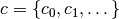 .
The weight factors
.
The weight factors  are given by
  where
where  is the experimental error on the data-point
 . The errors are assumed to be
Gaussian and uncorrelated.
For unweighted data the chi-squared sum is computed without any weight factors.
. The errors are assumed to be
Gaussian and uncorrelated.
For unweighted data the chi-squared sum is computed without any weight factors.
The fitting routines return the best-fit parameters  and their
 covariance matrix. The covariance matrix measures the
statistical errors on the best-fit parameters resulting from the
errors on the data, , and is defined
as
covariance matrix. The covariance matrix measures the
statistical errors on the best-fit parameters resulting from the
errors on the data, , and is defined
as
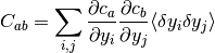
where  denotes an average over the Gaussian error distributions of the underlying datapoints.
The covariance matrix is calculated by error propagation from the data
errors . The change in a fitted parameter  caused by a small change in the data
  is given
by
is given
by
allowing the covariance matrix to be written in terms of the errors on the data,
For uncorrelated data the fluctuations of the underlying datapoints satisfy
giving a corresponding parameter covariance matrix of
When computing the covariance matrix for unweighted data, i.e. data with unknown errors,
the weight factors in this sum are replaced by the single estimate
 , where
  is the computed variance of the
residuals about the best-fit model,
is the computed variance of the
residuals about the best-fit model,  .
This is referred to as the variance-covariance matrix.
.
This is referred to as the variance-covariance matrix.
The standard deviations of the best-fit parameters are given by the
square root of the corresponding diagonal elements of
the covariance matrix,  .
The correlation coefficient of the fit parameters
.
The correlation coefficient of the fit parameters  and
and  is given by
  .
.
Linear regression
The functions in this section are used to fit simple one or two
parameter linear regression models. The functions are declared in
the header file gsl_fit.h.
Linear regression with a constant term
The functions described in this section can be used to perform
least-squares fits to a straight line model,  .
.
-
int gsl_fit_linear(const double *x, const size_t xstride, const double *y, const size_t ystride, size_t n, double *c0, double *c1, double *cov00, double *cov01, double *cov11, double *sumsq)
This function computes the best-fit linear regression coefficients (
c0,c1) of the model for the dataset
(
for the dataset
(x,y), two vectors of lengthnwith stridesxstrideandystride. The errors onyare assumed unknown so the variance-covariance matrix for the parameters (c0,c1) is estimated from the scatter of the points around the best-fit line and returned via the parameters (cov00,cov01,cov11). The sum of squares of the residuals from the best-fit line is returned insumsq. Note: the correlation coefficient of the data can be computed usinggsl_stats_correlation(), it does not depend on the fit.
-
int gsl_fit_wlinear(const double *x, const size_t xstride, const double *w, const size_t wstride, const double *y, const size_t ystride, size_t n, double *c0, double *c1, double *cov00, double *cov01, double *cov11, double *chisq)
This function computes the best-fit linear regression coefficients (
c0,c1) of the model for the weighted
dataset (x,y), two vectors of lengthnwith stridesxstrideandystride. The vectorw, of lengthnand stridewstride, specifies the weight of each datapoint. The weight is the reciprocal of the variance for each datapoint iny.The covariance matrix for the parameters (
c0,c1) is computed using the weights and returned via the parameters (cov00,cov01,cov11). The weighted sum of squares of the residuals from the best-fit line,, is returned in
chisq.
-
int gsl_fit_linear_est(double x, double c0, double c1, double cov00, double cov01, double cov11, double *y, double *y_err)
This function uses the best-fit linear regression coefficients
c0,c1and their covariancecov00,cov01,cov11to compute the fitted functionyand its standard deviationy_errfor the model
at the point x.
Linear regression without a constant term
The functions described in this section can be used to perform
least-squares fits to a straight line model without a constant term,
 .
.
-
int gsl_fit_mul(const double *x, const size_t xstride, const double *y, const size_t ystride, size_t n, double *c1, double *cov11, double *sumsq)
This function computes the best-fit linear regression coefficient
c1of the model for the datasets (x,y), two vectors of lengthnwith stridesxstrideandystride. The errors onyare assumed unknown so the variance of the parameterc1is estimated from the scatter of the points around the best-fit line and returned via the parametercov11. The sum of squares of the residuals from the best-fit line is returned insumsq.
-
int gsl_fit_wmul(const double *x, const size_t xstride, const double *w, const size_t wstride, const double *y, const size_t ystride, size_t n, double *c1, double *cov11, double *sumsq)
This function computes the best-fit linear regression coefficient
c1of the model for the weighted datasets
(x,y), two vectors of lengthnwith stridesxstrideandystride. The vectorw, of lengthnand stridewstride, specifies the weight of each datapoint. The weight is the reciprocal of the variance for each datapoint iny.The variance of the parameter
c1is computed using the weights and returned via the parametercov11. The weighted sum of squares of the residuals from the best-fit line,, is
returned in chisq.
Multi-parameter regression
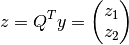
This section describes routines which perform least squares fits to a linear model by minimizing the cost function
where  is a vector of observations,
  is an
-by- matrix of predictor variables,
is a vector of the unknown best-fit parameters to be estimated,
and
is an
-by- matrix of predictor variables,
is a vector of the unknown best-fit parameters to be estimated,
and  .
The matrix
.
The matrix  defines the weights or uncertainties of the observation vector.
This formulation can be used for fits to any number of functions and/or
variables by preparing the -by- matrix
appropriately. For example, to fit to a -th order polynomial in
x, use the following matrix,

where the index  runs over the observations and the index
 runs from 0 to
  .
.
To fit to a set of sinusoidal functions with fixed frequencies
 ,
,  ,
,  ,
,  , use,
To fit to independent variables  ,
,  , ,
, ,
 , use,

where  is the -th value of the predictor variable
 .
.
The solution of the general linear least-squares system requires an
additional working space for intermediate results, such as the singular
value decomposition of the matrix .
These functions are declared in the header file gsl_multifit.h.
-
type gsl_multifit_linear_workspace
This workspace contains internal variables for fitting multi-parameter models.
-
gsl_multifit_linear_workspace *gsl_multifit_linear_alloc(const size_t n, const size_t p)
This function allocates a workspace for fitting a model to a maximum of
nobservations using a maximum ofpparameters. The user may later supply a smaller least squares system if desired. The size of the workspace is .
.
-
void gsl_multifit_linear_free(gsl_multifit_linear_workspace *work)
This function frees the memory associated with the workspace
w.
-
int gsl_multifit_linear_svd(const gsl_matrix *X, gsl_multifit_linear_workspace *work)
This function performs a singular value decomposition of the matrix
Xand stores the SVD factors internally inwork.
-
int gsl_multifit_linear_bsvd(const gsl_matrix *X, gsl_multifit_linear_workspace *work)
This function performs a singular value decomposition of the matrix
Xand stores the SVD factors internally inwork. The matrixXis first balanced by applying column scaling factors to improve the accuracy of the singular values.
-
int gsl_multifit_linear(const gsl_matrix *X, const gsl_vector *y, gsl_vector *c, gsl_matrix *cov, double *chisq, gsl_multifit_linear_workspace *work)
This function computes the best-fit parameters
cof the model for the observations
 yand the matrix of predictor variablesX, using the preallocated workspace provided inwork. The-by- variance-covariance matrix of the model parameters
covis set to , where
  is
the standard deviation of the fit residuals.
The sum of squares of the residuals from the best-fit,
, is returned in
is
the standard deviation of the fit residuals.
The sum of squares of the residuals from the best-fit,
, is returned in chisq. If the coefficient of determination is desired, it can be computed from the expression , where the total sum of squares (TSS) of
the observations
, where the total sum of squares (TSS) of
the observations ymay be computed fromgsl_stats_tss().The best-fit is found by singular value decomposition of the matrix
Xusing the modified Golub-Reinsch SVD algorithm, with column scaling to improve the accuracy of the singular values. Any components which have zero singular value (to machine precision) are discarded from the fit.
-
int gsl_multifit_linear_tsvd(const gsl_matrix *X, const gsl_vector *y, const double tol, gsl_vector *c, gsl_matrix *cov, double *chisq, size_t *rank, gsl_multifit_linear_workspace *work)
This function computes the best-fit parameters
cof the model for the observations yand the matrix of predictor variablesX, using a truncated SVD expansion. Singular values which satisfy are discarded from the fit, where
  is the largest singular value.
The -by- variance-covariance matrix of the model parameters
is the largest singular value.
The -by- variance-covariance matrix of the model parameters
covis set to, where is
the standard deviation of the fit residuals.
The sum of squares of the residuals from the best-fit,
, is returned in chisq. The effective rank (number of singular values used in solution) is returned inrank. If the coefficient of determination is desired, it can be computed from the expression, where the total sum of squares (TSS) of
the observations ymay be computed fromgsl_stats_tss().
-
int gsl_multifit_wlinear(const gsl_matrix *X, const gsl_vector *w, const gsl_vector *y, gsl_vector *c, gsl_matrix *cov, double *chisq, gsl_multifit_linear_workspace *work)
This function computes the best-fit parameters
cof the weighted model for the observations ywith weightswand the matrix of predictor variablesX, using the preallocated workspace provided inwork. The-by- covariance matrix of the model
parameters covis computed as . The weighted
sum of squares of the residuals from the best-fit, , is
returned in
. The weighted
sum of squares of the residuals from the best-fit, , is
returned in chisq. If the coefficient of determination is desired, it can be computed from the expression ,
where the weighted total sum of squares (WTSS) of the
observations
,
where the weighted total sum of squares (WTSS) of the
observations ymay be computed fromgsl_stats_wtss().
-
int gsl_multifit_wlinear_tsvd(const gsl_matrix *X, const gsl_vector *w, const gsl_vector *y, const double tol, gsl_vector *c, gsl_matrix *cov, double *chisq, size_t *rank, gsl_multifit_linear_workspace *work)
This function computes the best-fit parameters
cof the weighted model for the observations ywith weightswand the matrix of predictor variablesX, using a truncated SVD expansion. Singular values which satisfy
are discarded from the fit, where is the largest singular value.
The -by- covariance matrix of the model
parameters covis computed as. The weighted
sum of squares of the residuals from the best-fit, , is
returned in chisq. The effective rank of the system (number of singular values used in the solution) is returned inrank. If the coefficient of determination is desired, it can be computed from the expression,
where the weighted total sum of squares (WTSS) of the
observations ymay be computed fromgsl_stats_wtss().
-
int gsl_multifit_linear_est(const gsl_vector *x, const gsl_vector *c, const gsl_matrix *cov, double *y, double *y_err)
This function uses the best-fit multilinear regression coefficients
cand their covariance matrixcovto compute the fitted function valueyand its standard deviationy_errfor the model at the point
 x.
-
int gsl_multifit_linear_residuals(const gsl_matrix *X, const gsl_vector *y, const gsl_vector *c, gsl_vector *r)
This function computes the vector of residuals
 for
the observations
for
the observations y, coefficientscand matrix of predictor variablesX.
-
size_t gsl_multifit_linear_rank(const double tol, const gsl_multifit_linear_workspace *work)
This function returns the rank of the matrix
which must first have its
singular value decomposition computed. The rank is computed by counting the number
of singular values  which satisfy
  ,
where
,
where  is the largest singular value.
Regularized regression
Ordinary weighted least squares models seek a solution vector
which minimizes the residual
where is the -by- observation vector,
is the -by- design matrix, is
the -by- solution vector,
observation vector,
is the -by- design matrix, is
the -by- solution vector,
 is the data weighting matrix,
and .
In cases where the least squares matrix is ill-conditioned,
small perturbations (ie: noise) in the observation vector could lead to
widely different solution vectors .
One way of dealing with ill-conditioned matrices is to use a “truncated SVD”
in which small singular values, below some given tolerance, are discarded
from the solution. The truncated SVD method is available using the functions
is the data weighting matrix,
and .
In cases where the least squares matrix is ill-conditioned,
small perturbations (ie: noise) in the observation vector could lead to
widely different solution vectors .
One way of dealing with ill-conditioned matrices is to use a “truncated SVD”
in which small singular values, below some given tolerance, are discarded
from the solution. The truncated SVD method is available using the functions
gsl_multifit_linear_tsvd() and gsl_multifit_wlinear_tsvd(). Another way
to help solve ill-posed problems is to include a regularization term in the least squares
minimization

for a suitably chosen regularization parameter  and
matrix
and
matrix  . This type of regularization is known as Tikhonov, or ridge,
regression. In some applications, is chosen as the identity matrix, giving
preference to solution vectors with smaller norms.
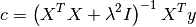
Including this regularization term leads to the explicit “normal equations” solution
. This type of regularization is known as Tikhonov, or ridge,
regression. In some applications, is chosen as the identity matrix, giving
preference to solution vectors with smaller norms.
Including this regularization term leads to the explicit “normal equations” solution
which reduces to the ordinary least squares solution when  .
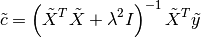
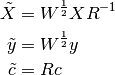
In practice, it is often advantageous to transform a regularized least
squares system into the form
.
In practice, it is often advantageous to transform a regularized least
squares system into the form
This is known as the Tikhonov “standard form” and has the normal equations solution
For an  -by- matrix which is full rank and has
  (ie: is
square or has more rows than columns), we can calculate the “thin” QR decomposition of , and
note that
(ie: is
square or has more rows than columns), we can calculate the “thin” QR decomposition of , and
note that  since the
  factor will not change the norm. Since
 is -by-, we can then use the transformation
to achieve the standard form. For a rectangular matrix with  ,
a more sophisticated approach is needed (see Hansen 1998, chapter 2.3).
In practice, the normal equations solution above is not desirable due to
numerical instabilities, and so the system is solved using the
singular value decomposition of the matrix
,
a more sophisticated approach is needed (see Hansen 1998, chapter 2.3).
In practice, the normal equations solution above is not desirable due to
numerical instabilities, and so the system is solved using the
singular value decomposition of the matrix  .
The matrix is often chosen as the identity matrix, or as a first
or second finite difference operator, to ensure a smoothly varying
coefficient vector , or as a diagonal matrix to selectively damp
each model parameter differently. If
.
The matrix is often chosen as the identity matrix, or as a first
or second finite difference operator, to ensure a smoothly varying
coefficient vector , or as a diagonal matrix to selectively damp
each model parameter differently. If  , the user must first
convert the least squares problem to standard form using
, the user must first
convert the least squares problem to standard form using
gsl_multifit_linear_stdform1() or gsl_multifit_linear_stdform2(),
solve the system, and then backtransform the solution vector to recover
the solution of the original problem (see
gsl_multifit_linear_genform1() and gsl_multifit_linear_genform2()).
In many regularization problems, care must be taken when choosing
the regularization parameter . Since both the
residual norm  and solution norm
  are being minimized, the parameter represents
a tradeoff between minimizing either the residuals or the
solution vector. A common tool for visualizing the comprimise between
the minimization of these two quantities is known as the L-curve.
The L-curve is a log-log plot of the residual norm
on the horizontal axis and the solution norm on the
vertical axis. This curve nearly always as an shaped
appearance, with a distinct corner separating the horizontal
and vertical sections of the curve. The regularization parameter
corresponding to this corner is often chosen as the optimal
value. GSL provides routines to calculate the L-curve for all
relevant regularization parameters as well as locating the corner.
are being minimized, the parameter represents
a tradeoff between minimizing either the residuals or the
solution vector. A common tool for visualizing the comprimise between
the minimization of these two quantities is known as the L-curve.
The L-curve is a log-log plot of the residual norm
on the horizontal axis and the solution norm on the
vertical axis. This curve nearly always as an shaped
appearance, with a distinct corner separating the horizontal
and vertical sections of the curve. The regularization parameter
corresponding to this corner is often chosen as the optimal
value. GSL provides routines to calculate the L-curve for all
relevant regularization parameters as well as locating the corner.
Another method of choosing the regularization parameter is known
as Generalized Cross Validation (GCV). This method is based on
the idea that if an arbitrary element is left out of the
right hand side, the resulting regularized solution should predict this element
accurately. This leads to choosing the parameter
which minimizes the GCV function
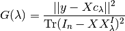
where  is the matrix which relates the solution
  to the right hand side , ie:
  . GSL
provides routines to compute the GCV curve and its minimum.
. GSL
provides routines to compute the GCV curve and its minimum.
For most applications, the steps required to solve a regularized least squares problem are as follows:
Construct the least squares system (
, ,  , )
, )Transform the system to standard form (
,  ). This
step can be skipped if
). This
step can be skipped if  and
and  .
.Calculate the SVD of
.Determine an appropriate regularization parameter
(using for example
L-curve or GCV analysis).Solve the standard form system using the chosen
and the SVD of .Backtransform the standard form solution
 to recover the
original solution vector .
to recover the
original solution vector .
-
int gsl_multifit_linear_stdform1(const gsl_vector *L, const gsl_matrix *X, const gsl_vector *y, gsl_matrix *Xs, gsl_vector *ys, gsl_multifit_linear_workspace *work)
-
int gsl_multifit_linear_wstdform1(const gsl_vector *L, const gsl_matrix *X, const gsl_vector *w, const gsl_vector *y, gsl_matrix *Xs, gsl_vector *ys, gsl_multifit_linear_workspace *work)
These functions define a regularization matrix
 .
The diagonal matrix element
.
The diagonal matrix element  is provided by the
-th element of the input vector
is provided by the
-th element of the input vector L. The-by- least squares matrix Xand vectoryof length are then
converted to standard form as described above and the parameters
(, ) are stored in Xsandyson output.Xsandyshave the same dimensions asXandy. Optional data weights may be supplied in the vectorwof length. In order to apply this transformation,
 must exist and so none of the
may be zero. After the standard form system has been solved,
use
must exist and so none of the
may be zero. After the standard form system has been solved,
use gsl_multifit_linear_genform1()to recover the original solution vector. It is allowed to haveX=Xsandy=ysfor an in-place transform. In order to perform a weighted regularized fit with , the user may
call
, the user may
call gsl_multifit_linear_applyW()to convert to standard form.
-
int gsl_multifit_linear_L_decomp(gsl_matrix *L, gsl_vector *tau)
This function factors the
-by- regularization matrix
Linto a form needed for the later transformation to standard form.Lmay have any number of rows. If  the QR decomposition of
Lis computed and stored inLon output. If, the QR decomposition
of  is computed and stored in
 Lon output. On output, the Householder scalars are stored in the vectortauof size .
These outputs will be used by
.
These outputs will be used by gsl_multifit_linear_wstdform2()to complete the transformation to standard form.
-
int gsl_multifit_linear_stdform2(const gsl_matrix *LQR, const gsl_vector *Ltau, const gsl_matrix *X, const gsl_vector *y, gsl_matrix *Xs, gsl_vector *ys, gsl_matrix *M, gsl_multifit_linear_workspace *work)
-
int gsl_multifit_linear_wstdform2(const gsl_matrix *LQR, const gsl_vector *Ltau, const gsl_matrix *X, const gsl_vector *w, const gsl_vector *y, gsl_matrix *Xs, gsl_vector *ys, gsl_matrix *M, gsl_multifit_linear_workspace *work)
These functions convert the least squares system (
X,y,W,) to standard
form (, ) which are stored in Xsandysrespectively. The-by- regularization matrix Lis specified by the inputsLQRandLtau, which are outputs fromgsl_multifit_linear_L_decomp(). The dimensions of the standard form parameters (, )
depend on whether is larger or less than . For ,
Xsis-by-, ysis-by-1, and Mis not used. For, Xsis -by-,
-by-,
ysis-by-1, and Mis additional-by- workspace,
which is required to recover the original solution vector after the system has been
solved (see gsl_multifit_linear_genform2()). Optional data weights may be supplied in the vectorwof length, where  .
.
-
int gsl_multifit_linear_solve(const double lambda, const gsl_matrix *Xs, const gsl_vector *ys, gsl_vector *cs, double *rnorm, double *snorm, gsl_multifit_linear_workspace *work)
This function computes the regularized best-fit parameters
which minimize the cost function
 which is in standard form. The least squares system must therefore be converted
to standard form prior to calling this function.
The observation vector is provided in
which is in standard form. The least squares system must therefore be converted
to standard form prior to calling this function.
The observation vector is provided in ysand the matrix of predictor variables in Xs. The solution vector is
returned in cs, which has length min( ). The SVD of
 Xsmust be computed prior to calling this function, usinggsl_multifit_linear_svd(). The regularization parameter is provided in lambda. The residual norm is returned in
 rnorm. The solution norm is returned in
snorm.
-
int gsl_multifit_linear_genform1(const gsl_vector *L, const gsl_vector *cs, gsl_vector *c, gsl_multifit_linear_workspace *work)
After a regularized system has been solved with
 ,
this function backtransforms the standard form solution vector
,
this function backtransforms the standard form solution vector csto recover the solution vector of the original problemc. The diagonal matrix elements are provided in
the vector L. It is allowed to havec=csfor an in-place transform.
-
int gsl_multifit_linear_genform2(const gsl_matrix *LQR, const gsl_vector *Ltau, const gsl_matrix *X, const gsl_vector *y, const gsl_vector *cs, const gsl_matrix *M, gsl_vector *c, gsl_multifit_linear_workspace *work)
-
int gsl_multifit_linear_wgenform2(const gsl_matrix *LQR, const gsl_vector *Ltau, const gsl_matrix *X, const gsl_vector *w, const gsl_vector *y, const gsl_vector *cs, const gsl_matrix *M, gsl_vector *c, gsl_multifit_linear_workspace *work)
After a regularized system has been solved with a general rectangular matrix
,
specified by (LQR,Ltau), this function backtransforms the standard form solutioncsto recover the solution vector of the original problem, which is stored inc, of length. The original least squares matrix and observation vector are provided in
Xandyrespectively.Mis the matrix computed bygsl_multifit_linear_stdform2(). For weighted fits, the weight vectorwmust also be supplied.
-
int gsl_multifit_linear_applyW(const gsl_matrix *X, const gsl_vector *w, const gsl_vector *y, gsl_matrix *WX, gsl_vector *Wy)
For weighted least squares systems with
, this function may be used to
convert the system to standard form by applying the weight matrix
to the least squares matrix Xand observation vectory. On output,WXis equal to and
and Wyis equal to . It is allowed
for
. It is allowed
for WX=XandWy=yfor an in-place transform.
-
int gsl_multifit_linear_lreg(const double smin, const double smax, gsl_vector *reg_param)
This function computes a set of possible regularization parameters for L-curve analysis and stores them in the output vector
reg_paramof length , where is
the number of desired points on the L-curve. The regularization parameters are equally logarithmically
distributed between the provided values
, where is
the number of desired points on the L-curve. The regularization parameters are equally logarithmically
distributed between the provided values sminandsmax, which typically correspond to the minimum and maximum singular value of the least squares matrix in standard form. The regularization parameters are calculated as,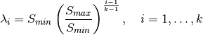
-
int gsl_multifit_linear_lcurve(const gsl_vector *y, gsl_vector *reg_param, gsl_vector *rho, gsl_vector *eta, gsl_multifit_linear_workspace *work)
This function computes the L-curve for a least squares system using the right hand side vector
yand the SVD decomposition of the least squares matrixX, which must be provided togsl_multifit_linear_svd()prior to calling this function. The output vectorsreg_param,rho, andetamust all be the same size, and will contain the regularization parameters , residual norms
 , and solution norms
  which compose the L-curve, where
  is the regularized
solution vector corresponding to .
The user may determine the number of points on the L-curve by
adjusting the size of these input arrays. The regularization
parameters are estimated from the singular values
of
is the regularized
solution vector corresponding to .
The user may determine the number of points on the L-curve by
adjusting the size of these input arrays. The regularization
parameters are estimated from the singular values
of X, and chosen to represent the most relevant portion of the L-curve.
-
int gsl_multifit_linear_lcurvature(const gsl_vector *y, const gsl_vector *reg_param, const gsl_vector *rho, const gsl_vector *eta, gsl_vector *kappa, gsl_multifit_linear_workspace *work)
This function computes the curvature of the L-curve
 , where
 and
and
 .
This function uses the right hand side vector
.
This function uses the right hand side vector y, the vector of regularization parameters,reg_param, vector of residual norms,rho, and vector of solution norms,eta. The arraysreg_param,rho, andetacan be computed bygsl_multifit_linear_lcurve(). The curvature is defined as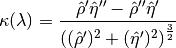
The curvature values are stored in
kappaon output. The functiongsl_multifit_linear_svd()must be called on the least squares matrix prior to calling this function.
-
int gsl_multifit_linear_lcurvature_menger(const gsl_vector *rho, const gsl_vector *eta, gsl_vector *kappa)
This function computes the Menger curvature of the L-curve
, where
and
.
The function computes the Menger curvature for each consecutive triplet of points,
 , where
  is the radius of the unique
circle fitted to the points
is the radius of the unique
circle fitted to the points
 .
.The vector of residual norms
 is provided in
 rho, the vector of solution norms is provided in
 eta. These arrays can be calculated by callinggsl_multifit_linear_lcurve(). The Menger curvature output is stored inkappa. The Menger curvature is an approximation to the curvature calculated bygsl_multifit_linear_lcurvature()but may be faster to calculate.
-
int gsl_multifit_linear_lcorner(const gsl_vector *rho, const gsl_vector *eta, size_t *idx)
This function attempts to locate the corner of the L-curve
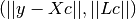 defined by the
 rhoandetainput arrays respectively. The corner is defined as the point of maximum curvature of the L-curve in log-log scale. Therhoandetaarrays can be outputs ofgsl_multifit_linear_lcurve(). The algorithm used simply fits a circle to 3 consecutive points on the L-curve and uses the circle’s radius to determine the curvature at the middle point. Therefore, the input array sizes must be . With more points provided for the L-curve, a better
estimate of the curvature can be obtained. The array index
corresponding to maximum curvature (ie: the corner) is returned
in
. With more points provided for the L-curve, a better
estimate of the curvature can be obtained. The array index
corresponding to maximum curvature (ie: the corner) is returned
in idx. If the input arrays contain colinear points, this function could fail and returnGSL_EINVAL.
-
int gsl_multifit_linear_lcorner2(const gsl_vector *reg_param, const gsl_vector *eta, size_t *idx)
This function attempts to locate the corner of an alternate L-curve
 studied by Rezghi and Hosseini, 2009.
This alternate L-curve can provide better estimates of the
regularization parameter for smooth solution vectors. The regularization
parameters and solution norms are provided
in the
studied by Rezghi and Hosseini, 2009.
This alternate L-curve can provide better estimates of the
regularization parameter for smooth solution vectors. The regularization
parameters and solution norms are provided
in the reg_paramandetainput arrays respectively. The corner is defined as the point of maximum curvature of this alternate L-curve in linear scale. Thereg_paramandetaarrays can be outputs ofgsl_multifit_linear_lcurve(). The algorithm used simply fits a circle to 3 consecutive points on the L-curve and uses the circle’s radius to determine the curvature at the middle point. Therefore, the input array sizes must be. With more points provided for the L-curve, a better
estimate of the curvature can be obtained. The array index
corresponding to maximum curvature (ie: the corner) is returned
in idx. If the input arrays contain colinear points, this function could fail and returnGSL_EINVAL.
-
int gsl_multifit_linear_gcv_init(const gsl_vector *y, gsl_vector *reg_param, gsl_vector *UTy, double *delta0, gsl_multifit_linear_workspace *work)
This function performs some initialization in preparation for computing the GCV curve and its minimum. The right hand side vector is provided in
y. On output,reg_paramis set to a vector of regularization parameters in decreasing order and may be of any size. The vectorUTyof size is set to  . The parameter
delta0is needed for subsequent steps of the GCV calculation.
-
int gsl_multifit_linear_gcv_curve(const gsl_vector *reg_param, const gsl_vector *UTy, const double delta0, gsl_vector *G, gsl_multifit_linear_workspace *work)
This funtion calculates the GCV curve
 and stores it in
Gon output, which must be the same size asreg_param. The inputsreg_param,UTyanddelta0are computed ingsl_multifit_linear_gcv_init().
-
int gsl_multifit_linear_gcv_min(const gsl_vector *reg_param, const gsl_vector *UTy, const gsl_vector *G, const double delta0, double *lambda, gsl_multifit_linear_workspace *work)
This function computes the value of the regularization parameter which minimizes the GCV curve
and stores it in
lambda. The inputGis calculated bygsl_multifit_linear_gcv_curve()and the inputsreg_param,UTyanddelta0are computed bygsl_multifit_linear_gcv_init().
-
double gsl_multifit_linear_gcv_calc(const double lambda, const gsl_vector *UTy, const double delta0, gsl_multifit_linear_workspace *work)
This function returns the value of the GCV curve
corresponding
to the input lambda.
-
int gsl_multifit_linear_gcv(const gsl_vector *y, gsl_vector *reg_param, gsl_vector *G, double *lambda, double *G_lambda, gsl_multifit_linear_workspace *work)
This function combines the steps
gcv_init,gcv_curve, andgcv_mindefined above into a single function. The inputyis the right hand side vector. On output,reg_paramandG, which must be the same size, are set to vectors of and values respectively. The
output lambdais set to the optimal value of
which minimizes the GCV curve. The minimum value of the GCV curve is
returned in G_lambda.
-
int gsl_multifit_linear_Lk(const size_t p, const size_t k, gsl_matrix *L)
This function computes the discrete approximation to the derivative operator
 of
order
of
order kon a regular grid ofppoints and stores it inL. The dimensions ofLare -by-.
-by-.
-
int gsl_multifit_linear_Lsobolev(const size_t p, const size_t kmax, const gsl_vector *alpha, gsl_matrix *L, gsl_multifit_linear_workspace *work)
This function computes the regularization matrix
Lcorresponding to the weighted Sobolov norm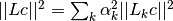 where approximates
the derivative operator of order . This regularization norm can be useful
in applications where it is necessary to smooth several derivatives of the solution.
where approximates
the derivative operator of order . This regularization norm can be useful
in applications where it is necessary to smooth several derivatives of the solution.
pis the number of model parameters,kmaxis the highest derivative to include in the summation above, andalphais the vector of weights of sizekmax+ 1, wherealpha[k]= is the weight
assigned to the derivative of order . The output matrix
is the weight
assigned to the derivative of order . The output matrix Lis sizep-by-pand upper triangular.
-
double gsl_multifit_linear_rcond(const gsl_multifit_linear_workspace *work)
This function returns the reciprocal condition number of the least squares matrix
,
defined as the ratio of the smallest and largest singular values,
rcond =  .
The routine
.
The routine gsl_multifit_linear_svd()must first be called to compute the SVD of.
Robust linear regression
Ordinary least squares (OLS) models are often heavily influenced by the presence of outliers. Outliers are data points which do not follow the general trend of the other observations, although there is strictly no precise definition of an outlier. Robust linear regression refers to regression algorithms which are robust to outliers. The most common type of robust regression is M-estimation. The general M-estimator minimizes the objective function
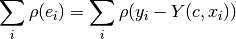
where  is the residual of the ith data point, and
 is a function which should have the following properties:


 for
for 
The special case of ordinary least squares is given by  .
Letting
.
Letting  be the derivative of
  , differentiating
the objective function with respect to the coefficients
and setting the partial derivatives to zero produces the system of equations
, differentiating
the objective function with respect to the coefficients
and setting the partial derivatives to zero produces the system of equations
where  is a vector containing row of the design matrix .
Next, we define a weight function
is a vector containing row of the design matrix .
Next, we define a weight function  , and let
 :
:
This system of equations is equivalent to solving a weighted ordinary least squares
problem, minimizing  . The weights however, depend
on the residuals
. The weights however, depend
on the residuals  , which depend on the coefficients , which depend
on the weights. Therefore, an iterative solution is used, called Iteratively Reweighted
Least Squares (IRLS).
, which depend on the coefficients , which depend
on the weights. Therefore, an iterative solution is used, called Iteratively Reweighted
Least Squares (IRLS).
Compute initial estimates of the coefficients
 using ordinary least squares
For iteration
, form the residuals  ,
where
,
where  is a tuning constant depending on the choice of
  , and
, and  are the
statistical leverages (diagonal elements of the matrix
are the
statistical leverages (diagonal elements of the matrix  ). Including
and in the residual calculation has been shown to improve the convergence of the method.
The residual standard deviation is approximated as
). Including
and in the residual calculation has been shown to improve the convergence of the method.
The residual standard deviation is approximated as  , where MAD is the
Median-Absolute-Deviation of the
, where MAD is the
Median-Absolute-Deviation of the  largest residuals from the previous iteration.
Compute new weights
 .
.Compute new coefficients
 by solving the weighted least squares problem with
weights
by solving the weighted least squares problem with
weights  .
.Steps 2 through 4 are iterated until the coefficients converge or until some maximum iteration limit is reached. Coefficients are tested for convergence using the critera:
for all
where
is a small tolerance factor.

The key to this method lies in selecting the function  to assign
smaller weights to large residuals, and larger weights to smaller residuals. As
the iteration proceeds, outliers are assigned smaller and smaller weights, eventually
having very little or no effect on the fitted model.
to assign
smaller weights to large residuals, and larger weights to smaller residuals. As
the iteration proceeds, outliers are assigned smaller and smaller weights, eventually
having very little or no effect on the fitted model.
-
type gsl_multifit_robust_workspace
This workspace is used for robust least squares fitting.
-
gsl_multifit_robust_workspace *gsl_multifit_robust_alloc(const gsl_multifit_robust_type *T, const size_t n, const size_t p)
This function allocates a workspace for fitting a model to
nobservations usingpparameters. The size of the workspace is. The type Tspecifies the function and can be selected from the following choices.-
type gsl_multifit_robust_type
-
gsl_multifit_robust_type *gsl_multifit_robust_default
This specifies the
gsl_multifit_robust_bisquaretype (see below) and is a good general purpose choice for robust regression.
-
gsl_multifit_robust_type *gsl_multifit_robust_bisquare
This is Tukey’s biweight (bisquare) function and is a good general purpose choice for robust regression. The weight function is given by
and the default tuning constant is
 .
.
-
gsl_multifit_robust_type *gsl_multifit_robust_cauchy
This is Cauchy’s function, also known as the Lorentzian function. This function does not guarantee a unique solution, meaning different choices of the coefficient vector
ccould minimize the objective function. Therefore this option should be used with care. The weight function is given by
and the default tuning constant is
 .
.
-
gsl_multifit_robust_type *gsl_multifit_robust_fair
This is the fair
function, which guarantees a unique solution and
has continuous derivatives to three orders. The weight function is given by
and the default tuning constant is
 .
.
-
gsl_multifit_robust_type *gsl_multifit_robust_huber
This specifies Huber’s
function, which is a parabola in the vicinity of zero and
increases linearly for a given threshold  . This function is also considered
an excellent general purpose robust estimator, however, occasional difficulties can
be encountered due to the discontinuous first derivative of the function.
The weight function is given by
. This function is also considered
an excellent general purpose robust estimator, however, occasional difficulties can
be encountered due to the discontinuous first derivative of the function.
The weight function is given by
and the default tuning constant is
 .
.
-
gsl_multifit_robust_type *gsl_multifit_robust_ols
This specifies the ordinary least squares solution, which can be useful for quickly checking the difference between the various robust and OLS solutions. The weight function is given by

and the default tuning constant is
 .
.
-
gsl_multifit_robust_type *gsl_multifit_robust_welsch
This specifies the Welsch function which can perform well in cases where the residuals have an exponential distribution. The weight function is given by
and the default tuning constant is
 .
.
-
gsl_multifit_robust_type *gsl_multifit_robust_default
-
type gsl_multifit_robust_type
-
void gsl_multifit_robust_free(gsl_multifit_robust_workspace *w)
This function frees the memory associated with the workspace
w.
-
const char *gsl_multifit_robust_name(const gsl_multifit_robust_workspace *w)
This function returns the name of the robust type
Tspecified togsl_multifit_robust_alloc().
-
int gsl_multifit_robust_tune(const double tune, gsl_multifit_robust_workspace *w)
This function sets the tuning constant
used to adjust the residuals at each
iteration to tune. Decreasing the tuning constant increases the downweight assigned to large residuals, while increasing the tuning constant decreases the downweight assigned to large residuals.
-
int gsl_multifit_robust_maxiter(const size_t maxiter, gsl_multifit_robust_workspace *w)
This function sets the maximum number of iterations in the iteratively reweighted least squares algorithm to
maxiter. By default, this value is set to 100 bygsl_multifit_robust_alloc().
-
int gsl_multifit_robust_weights(const gsl_vector *r, gsl_vector *wts, gsl_multifit_robust_workspace *w)
This function assigns weights to the vector
wtsusing the residual vectorrand previously specified weighting function. The output weights are given by , where the weighting functions
  are
detailed in
are
detailed in gsl_multifit_robust_alloc(). is an estimate of the
residual standard deviation based on the Median-Absolute-Deviation and
is the tuning constant. This function is useful if the user wishes to implement
their own robust regression rather than using
the supplied gsl_multifit_robust()routine below.
-
int gsl_multifit_robust(const gsl_matrix *X, const gsl_vector *y, gsl_vector *c, gsl_matrix *cov, gsl_multifit_robust_workspace *w)
This function computes the best-fit parameters
cof the model for the observations yand the matrix of predictor variablesX, attemping to reduce the influence of outliers using the algorithm outlined above. The-by- variance-covariance matrix of the model parameters
covis estimated as, where is
an approximation of the residual standard deviation using the theory of robust
regression. Special care must be taken when estimating and
other statistics such as  , and so these
are computed internally and are available by calling the function
, and so these
are computed internally and are available by calling the function
gsl_multifit_robust_statistics().If the coefficients do not converge within the maximum iteration limit, the function returns
GSL_EMAXITER. In this case, the current estimates of the coefficients and covariance matrix are returned incandcovand the internal fit statistics are computed with these estimates.
-
int gsl_multifit_robust_est(const gsl_vector *x, const gsl_vector *c, const gsl_matrix *cov, double *y, double *y_err)
This function uses the best-fit robust regression coefficients
cand their covariance matrixcovto compute the fitted function valueyand its standard deviationy_errfor the model at the point
 x.
-
int gsl_multifit_robust_residuals(const gsl_matrix *X, const gsl_vector *y, const gsl_vector *c, gsl_vector *r, gsl_multifit_robust_workspace *w)
This function computes the vector of studentized residuals
 for
the observations
for
the observations y, coefficientscand matrix of predictor variablesX. The routinegsl_multifit_robust()must first be called to compute the statisical leverages of
the matrix Xand residual standard deviation estimate.
-
gsl_multifit_robust_stats gsl_multifit_robust_statistics(const gsl_multifit_robust_workspace *w)
This function returns a structure containing relevant statistics from a robust regression. The function
gsl_multifit_robust()must be called first to perform the regression and calculate these statistics. The returnedgsl_multifit_robust_statsstructure contains the following fields.-
type gsl_multifit_robust_stats
double sigma_olsThis contains the standard deviation of the residuals as computed from ordinary least squares (OLS).
double sigma_madThis contains an estimate of the standard deviation of the final residuals using the Median-Absolute-Deviation statistic
double sigma_robThis contains an estimate of the standard deviation of the final residuals from the theory of robust regression (see Street et al, 1988).
double sigmaThis contains an estimate of the standard deviation of the final residuals by attemping to reconcile
sigma_robandsigma_olsin a reasonable way.double RsqThis contains the
coefficient of determination statistic using
the estimate sigma.double adj_RsqThis contains the adjusted
coefficient of determination statistic
using the estimate sigma.double rmseThis contains the root mean squared error of the final residuals
double sseThis contains the residual sum of squares taking into account the robust covariance matrix.
size_t dofThis contains the number of degrees of freedom

size_t numitUpon successful convergence, this contains the number of iterations performed
gsl_vector * weightsThis contains the final weight vector of length
ngsl_vector * rThis contains the final residual vector of length
n,
-
type gsl_multifit_robust_stats
Large dense linear systems
This module is concerned with solving large dense least squares systems
 where the -by- matrix
has
where the -by- matrix
has  (ie: many more rows than columns).
This type of matrix is called a “tall skinny” matrix, and for
some applications, it may not be possible to fit the
entire matrix in memory at once to use the standard SVD approach.
Therefore, the algorithms in this module are designed to allow
the user to construct smaller blocks of the matrix and
accumulate those blocks into the larger system one at a time. The
algorithms in this module never need to store the entire matrix
in memory. The large linear least squares routines
support data weights and Tikhonov regularization, and are
designed to minimize the residual
(ie: many more rows than columns).
This type of matrix is called a “tall skinny” matrix, and for
some applications, it may not be possible to fit the
entire matrix in memory at once to use the standard SVD approach.
Therefore, the algorithms in this module are designed to allow
the user to construct smaller blocks of the matrix and
accumulate those blocks into the larger system one at a time. The
algorithms in this module never need to store the entire matrix
in memory. The large linear least squares routines
support data weights and Tikhonov regularization, and are
designed to minimize the residual
where is the -by- observation vector,
is the -by- design matrix, is
the -by- solution vector,
is the data weighting matrix,
is an -by- regularization matrix,
is a regularization parameter,
and . In the discussion which follows,
we will assume that the system has been converted into Tikhonov
standard form,
and we will drop the tilde characters from the various parameters. For a discussion of the transformation to standard form, see Regularized regression.
The basic idea is to partition the matrix and observation
vector as
into blocks, where each block ( ) may have
any number of rows, but each has columns.
The sections below describe the methods available for solving
this partitioned system. The functions are declared in
the header file
) may have
any number of rows, but each has columns.
The sections below describe the methods available for solving
this partitioned system. The functions are declared in
the header file gsl_multilarge.h.
Normal Equations Approach
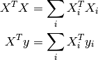
The normal equations approach to the large linear least squares problem described above is popular due to its speed and simplicity. Since the normal equations solution to the problem is given by
only the -by- matrix  and
-by-1 vector
and
-by-1 vector  need to be stored. Using
the partition scheme described above, these are given by
need to be stored. Using
the partition scheme described above, these are given by
Since the matrix is symmetric, only half of it
needs to be calculated. Once all of the blocks  have been accumulated into the final and ,
the system can be solved with a Cholesky factorization of the
matrix. The matrix is first transformed via
a diagonal scaling transformation to attempt to reduce its condition
number as much as possible to recover a more accurate solution vector.
The normal equations approach is the fastest method for solving the
large least squares problem, and is accurate for well-conditioned
matrices . However, for ill-conditioned matrices, as is often
the case for large systems, this method can suffer from numerical
instabilities (see Trefethen and Bau, 1997). The number of operations
for this method is
have been accumulated into the final and ,
the system can be solved with a Cholesky factorization of the
matrix. The matrix is first transformed via
a diagonal scaling transformation to attempt to reduce its condition
number as much as possible to recover a more accurate solution vector.
The normal equations approach is the fastest method for solving the
large least squares problem, and is accurate for well-conditioned
matrices . However, for ill-conditioned matrices, as is often
the case for large systems, this method can suffer from numerical
instabilities (see Trefethen and Bau, 1997). The number of operations
for this method is 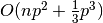 .
.
Tall Skinny QR (TSQR) Approach
An algorithm which has better numerical stability for ill-conditioned problems is known as the Tall Skinny QR (TSQR) method. This method is based on computing the QR decomposition of the least squares matrix,

where is an -by- orthogonal matrix,
and is a -by- upper triangular matrix.
If we define,
where  is -by-1 and
  is
is  -by-1,
then the residual becomes
-by-1,
then the residual becomes
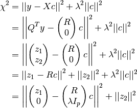
Since does not depend on , is minimized
by solving the least squares system,
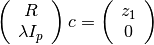
The matrix on the left hand side is now a much
smaller  -by- matrix which can
be solved with a standard SVD approach. The
matrix is large, however it does not need to be
explicitly constructed. The TSQR algorithm
computes only the -by- matrix
, the -by-1 vector ,
and the norm
-by- matrix which can
be solved with a standard SVD approach. The
matrix is large, however it does not need to be
explicitly constructed. The TSQR algorithm
computes only the -by- matrix
, the -by-1 vector ,
and the norm  ,
and updates these quantities as new blocks
are added to the system. Each time a new block of rows
() is added, the algorithm performs a QR decomposition
of the matrix
,
and updates these quantities as new blocks
are added to the system. Each time a new block of rows
() is added, the algorithm performs a QR decomposition
of the matrix

where  is the upper triangular
factor for the matrix
is the upper triangular
factor for the matrix

This QR decomposition is done efficiently taking into account
the sparse structure of . See Demmel et al, 2008 for
more details on how this is accomplished. The number
of operations for this method is 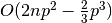 .
.
Large Dense Linear Systems Solution Steps
The typical steps required to solve large regularized linear least squares problems are as follows:
Choose the regularization matrix
.Construct a block of rows of the least squares matrix, right hand side vector, and weight vector (
, , ).Transform the block to standard form (
 ,
,  ). This
step can be skipped if and
). This
step can be skipped if and  .
.Accumulate the standard form block (
, ) into
the system.Repeat steps 2-4 until the entire matrix and right hand side vector have been accumulated.
Determine an appropriate regularization parameter
(using for example
L-curve analysis).Solve the standard form system using the chosen
.Backtransform the standard form solution
to recover the
original solution vector .
Large Dense Linear Least Squares Routines
-
type gsl_multilarge_linear_workspace
This workspace contains parameters for solving large linear least squares problems.
-
gsl_multilarge_linear_workspace *gsl_multilarge_linear_alloc(const gsl_multilarge_linear_type *T, const size_t p)
This function allocates a workspace for solving large linear least squares systems. The least squares matrix
has pcolumns, but may have any number of rows.-
type gsl_multilarge_linear_type
The parameter
Tspecifies the method to be used for solving the large least squares system and may be selected from the following choices-
gsl_multilarge_linear_type *gsl_multilarge_linear_normal
This specifies the normal equations approach for solving the least squares system. This method is suitable in cases where performance is critical and it is known that the least squares matrix
is well conditioned. The size
of this workspace is  .
.
-
gsl_multilarge_linear_type *gsl_multilarge_linear_tsqr
This specifies the sequential Tall Skinny QR (TSQR) approach for solving the least squares system. This method is a good general purpose choice for large systems, but requires about twice as many operations as the normal equations method for
. The size of this workspace is .
-
gsl_multilarge_linear_type *gsl_multilarge_linear_normal
-
type gsl_multilarge_linear_type
-
void gsl_multilarge_linear_free(gsl_multilarge_linear_workspace *w)
This function frees the memory associated with the workspace
w.
-
const char *gsl_multilarge_linear_name(gsl_multilarge_linear_workspace *w)
This function returns a string pointer to the name of the multilarge solver.
-
int gsl_multilarge_linear_reset(gsl_multilarge_linear_workspace *w)
This function resets the workspace
wso it can begin to accumulate a new least squares system.
-
int gsl_multilarge_linear_stdform1(const gsl_vector *L, const gsl_matrix *X, const gsl_vector *y, gsl_matrix *Xs, gsl_vector *ys, gsl_multilarge_linear_workspace *work)
-
int gsl_multilarge_linear_wstdform1(const gsl_vector *L, const gsl_matrix *X, const gsl_vector *w, const gsl_vector *y, gsl_matrix *Xs, gsl_vector *ys, gsl_multilarge_linear_workspace *work)
These functions define a regularization matrix
.
The diagonal matrix element is provided by the
-th element of the input vector L. The block (X,y) is converted to standard form and the parameters (, ) are stored in Xsandyson output.Xsandyshave the same dimensions asXandy. Optional data weights may be supplied in the vectorw. In order to apply this transformation, must exist and so none of the
may be zero. After the standard form system has been solved,
use gsl_multilarge_linear_genform1()to recover the original solution vector. It is allowed to haveX=Xsandy=ysfor an in-place transform.
-
int gsl_multilarge_linear_L_decomp(gsl_matrix *L, gsl_vector *tau)
This function calculates the QR decomposition of the
-by-
regularization matrix L.Lmust have. On output,
the Householder scalars are stored in the vector tauof size.
These outputs will be used by gsl_multilarge_linear_wstdform2()to complete the transformation to standard form.
-
int gsl_multilarge_linear_stdform2(const gsl_matrix *LQR, const gsl_vector *Ltau, const gsl_matrix *X, const gsl_vector *y, gsl_matrix *Xs, gsl_vector *ys, gsl_multilarge_linear_workspace *work)
-
int gsl_multilarge_linear_wstdform2(const gsl_matrix *LQR, const gsl_vector *Ltau, const gsl_matrix *X, const gsl_vector *w, const gsl_vector *y, gsl_matrix *Xs, gsl_vector *ys, gsl_multilarge_linear_workspace *work)
These functions convert a block of rows (
X,y,w) to standard form (, ) which are stored in Xsandysrespectively.X,y, andwmust all have the same number of rows. The-by- regularization matrix Lis specified by the inputsLQRandLtau, which are outputs fromgsl_multilarge_linear_L_decomp().Xsandyshave the same dimensions asXandy. After the standard form system has been solved, usegsl_multilarge_linear_genform2()to recover the original solution vector. Optional data weights may be supplied in the vectorw, where.
-
int gsl_multilarge_linear_accumulate(gsl_matrix *X, gsl_vector *y, gsl_multilarge_linear_workspace *w)
This function accumulates the standard form block (
 ) into the
current least squares system.
) into the
current least squares system. Xandyhave the same number of rows, which can be arbitrary.Xmust have columns.
For the TSQR method, Xandyare destroyed on output. For the normal equations method, they are both unchanged.
-
int gsl_multilarge_linear_solve(const double lambda, gsl_vector *c, double *rnorm, double *snorm, gsl_multilarge_linear_workspace *w)
After all blocks (
) have been accumulated into
the large least squares system, this function will compute
the solution vector which is stored in con output. The regularization parameter is provided in
lambda. On output,rnormcontains the residual norm and
and snormcontains the solution norm.
-
int gsl_multilarge_linear_genform1(const gsl_vector *L, const gsl_vector *cs, gsl_vector *c, gsl_multilarge_linear_workspace *work)
After a regularized system has been solved with
,
this function backtransforms the standard form solution vector csto recover the solution vector of the original problemc. The diagonal matrix elements are provided in
the vector L. It is allowed to havec=csfor an in-place transform.
-
int gsl_multilarge_linear_genform2(const gsl_matrix *LQR, const gsl_vector *Ltau, const gsl_vector *cs, gsl_vector *c, gsl_multilarge_linear_workspace *work)
After a regularized system has been solved with a regularization matrix
,
specified by (LQR,Ltau), this function backtransforms the standard form solutioncsto recover the solution vector of the original problem, which is stored inc, of length.
-
int gsl_multilarge_linear_lcurve(gsl_vector *reg_param, gsl_vector *rho, gsl_vector *eta, gsl_multilarge_linear_workspace *work)
This function computes the L-curve for a large least squares system after it has been fully accumulated into the workspace
work. The output vectorsreg_param,rho, andetamust all be the same size, and will contain the regularization parameters, residual norms , and solution
norms which compose the L-curve, where
is the regularized solution vector corresponding to .
The user may determine the number of points on the L-curve by
adjusting the size of these input arrays. For the TSQR method,
the regularization parameters are estimated from the
singular values of the triangular factor. For the normal
equations method, they are estimated from the eigenvalues of the
matrix.
-
const gsl_matrix *gsl_multilarge_linear_matrix_ptr(const gsl_multilarge_linear_workspace *work)
For the normal equations method, this function returns a pointer to the
matrix
of size -by-. For the TSQR method, this function returns a pointer to the
upper triangular matrix of size -by-.
-
const gsl_vector *gsl_multilarge_linear_rhs_ptr(const gsl_multilarge_linear_workspace *work)
For the normal equations method, this function returns a pointer to the
-by-1 right hand
side vector . For the TSQR method, this function returns a pointer to a vector of length
 . The first elements of this vector contain , while the last element
contains .
. The first elements of this vector contain , while the last element
contains .
-
int gsl_multilarge_linear_rcond(double *rcond, gsl_multilarge_linear_workspace *work)
This function computes the reciprocal condition number, stored in
rcond, of the least squares matrix after it has been accumulated into the workspacework. For the TSQR algorithm, this is accomplished by calculating the SVD of the factor, which
has the same singular values as the matrix . For the normal
equations method, this is done by computing the eigenvalues of
, which could be inaccurate for ill-conditioned matrices
.
Troubleshooting
When using models based on polynomials, care should be taken when constructing the design matrix
. If the  values are large, then the matrix could be ill-conditioned
since its columns are powers of , leading to unstable least-squares solutions.
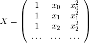
In this case it can often help to center and scale the values using the mean and standard deviation:
values are large, then the matrix could be ill-conditioned
since its columns are powers of , leading to unstable least-squares solutions.
In this case it can often help to center and scale the values using the mean and standard deviation:
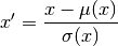
and then construct the matrix using the transformed values  .
.
Examples
The example programs in this section demonstrate the various linear regression methods.
Simple Linear Regression Example
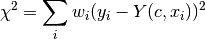
The following program computes a least squares straight-line fit to a simple dataset, and outputs the best-fit line and its associated one standard-deviation error bars.
#include <stdio.h>
#include <gsl/gsl_fit.h>

int
main (void)
{
  int i, n = 4;
  double x[4] = { 1970, 1980, 1990, 2000 };
  double y[4] = {   12,   11,   14,   13 };
  double w[4] = {  0.1,  0.2,  0.3,  0.4 };

  double c0, c1, cov00, cov01, cov11, chisq;

  gsl_fit_wlinear (x, 1, w, 1, y, 1, n,
                   &c0, &c1, &cov00, &cov01, &cov11,
                   &chisq);

  printf ("# best fit: Y = %g + %g X\n", c0, c1);
  printf ("# covariance matrix:\n");
  printf ("# [ %g, %g\n#   %g, %g]\n",
          cov00, cov01, cov01, cov11);
  printf ("# chisq = %g\n", chisq);

  for (i = 0; i < n; i++)
    printf ("data: %g %g %g\n",
                   x[i], y[i], 1/sqrt(w[i]));

  printf ("\n");

  for (i = -30; i < 130; i++)
    {
      double xf = x[0] + (i/100.0) * (x[n-1] - x[0]);
      double yf, yf_err;

      gsl_fit_linear_est (xf,
                          c0, c1,
                          cov00, cov01, cov11,
                          &yf, &yf_err);

      printf ("fit: %g %g\n", xf, yf);
      printf ("hi : %g %g\n", xf, yf + yf_err);
      printf ("lo : %g %g\n", xf, yf - yf_err);
    }
  return 0;
}
The following commands extract the data from the output of the program and display it using the GNU plotutils “graph” utility:
$ ./demo > tmp
$ more tmp
# best fit: Y = -106.6 + 0.06 X
# covariance matrix:
# [ 39602, -19.9
#   -19.9, 0.01]
# chisq = 0.8

$ for n in data fit hi lo ;
   do
     grep "^$n" tmp | cut -d: -f2 > $n ;
   done
$ graph -T X -X x -Y y -y 0 20 -m 0 -S 2 -Ie data
     -S 0 -I a -m 1 fit -m 2 hi -m 2 lo
The result is shown in Fig. 30.
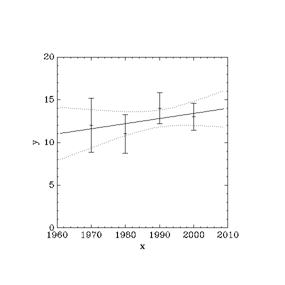
Fig. 30 Straight line fit with 1- error bars
Multi-parameter Linear Regression Example
The following program performs a quadratic fit 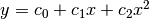 to a weighted dataset using the generalised linear fitting function
gsl_multifit_wlinear(). The model matrix for a quadratic
fit is given by,
where the column of ones corresponds to the constant term  .
The two remaining columns corresponds to the terms
.
The two remaining columns corresponds to the terms  and
and
 .
.
The program reads n lines of data in the format (x, y,
err) where err is the error (standard deviation) in the
value y.
#include <stdio.h>
#include <gsl/gsl_multifit.h>

int
main (int argc, char **argv)
{
  int i, n;
  double xi, yi, ei, chisq;
  gsl_matrix *X, *cov;
  gsl_vector *y, *w, *c;

  if (argc != 2)
    {
      fprintf (stderr,"usage: fit n < data\n");
      exit (-1);
    }

  n = atoi (argv[1]);

  X = gsl_matrix_alloc (n, 3);
  y = gsl_vector_alloc (n);
  w = gsl_vector_alloc (n);

  c = gsl_vector_alloc (3);
  cov = gsl_matrix_alloc (3, 3);

  for (i = 0; i < n; i++)
    {
      int count = fscanf (stdin, "%lg %lg %lg",
                          &xi, &yi, &ei);

      if (count != 3)
        {
          fprintf (stderr, "error reading file\n");
          exit (-1);
        }

      printf ("%g %g +/- %g\n", xi, yi, ei);

      gsl_matrix_set (X, i, 0, 1.0);
      gsl_matrix_set (X, i, 1, xi);
      gsl_matrix_set (X, i, 2, xi*xi);

      gsl_vector_set (y, i, yi);
      gsl_vector_set (w, i, 1.0/(ei*ei));
    }

  {
    gsl_multifit_linear_workspace * work
      = gsl_multifit_linear_alloc (n, 3);
    gsl_multifit_wlinear (X, w, y, c, cov,
                          &chisq, work);
    gsl_multifit_linear_free (work);
  }

#define C(i) (gsl_vector_get(c,(i)))
#define COV(i,j) (gsl_matrix_get(cov,(i),(j)))

  {
    printf ("# best fit: Y = %g + %g X + %g X^2\n",
            C(0), C(1), C(2));

    printf ("# covariance matrix:\n");
    printf ("[ %+.5e, %+.5e, %+.5e  \n",
               COV(0,0), COV(0,1), COV(0,2));
    printf ("  %+.5e, %+.5e, %+.5e  \n",
               COV(1,0), COV(1,1), COV(1,2));
    printf ("  %+.5e, %+.5e, %+.5e ]\n",
               COV(2,0), COV(2,1), COV(2,2));
    printf ("# chisq = %g\n", chisq);
  }

  gsl_matrix_free (X);
  gsl_vector_free (y);
  gsl_vector_free (w);
  gsl_vector_free (c);
  gsl_matrix_free (cov);

  return 0;
}
A suitable set of data for fitting can be generated using the following
program. It outputs a set of points with gaussian errors from the curve
 in the region
  .
.
#include <stdio.h>
#include <math.h>
#include <gsl/gsl_randist.h>

int
main (void)
{
  double x;
  const gsl_rng_type * T;
  gsl_rng * r;

  gsl_rng_env_setup ();

  T = gsl_rng_default;
  r = gsl_rng_alloc (T);

  for (x = 0.1; x < 2; x+= 0.1)
    {
      double y0 = exp (x);
      double sigma = 0.1 * y0;
      double dy = gsl_ran_gaussian (r, sigma);

      printf ("%g %g %g\n", x, y0 + dy, sigma);
    }

  gsl_rng_free(r);

  return 0;
}
The data can be prepared by running the resulting executable program:
$ GSL_RNG_TYPE=mt19937_1999 ./generate > exp.dat
$ more exp.dat
0.1 0.97935 0.110517
0.2 1.3359 0.12214
0.3 1.52573 0.134986
0.4 1.60318 0.149182
0.5 1.81731 0.164872
0.6 1.92475 0.182212
....
To fit the data use the previous program, with the number of data points given as the first argument. In this case there are 19 data points:
$ ./fit 19 < exp.dat
0.1 0.97935 +/- 0.110517
0.2 1.3359 +/- 0.12214
...
# best fit: Y = 1.02318 + 0.956201 X + 0.876796 X^2
# covariance matrix:
[ +1.25612e-02, -3.64387e-02, +1.94389e-02
  -3.64387e-02, +1.42339e-01, -8.48761e-02
  +1.94389e-02, -8.48761e-02, +5.60243e-02 ]
# chisq = 23.0987
The parameters of the quadratic fit match the coefficients of the
expansion of  , taking into account the errors on the
parameters and the
, taking into account the errors on the
parameters and the  difference between the exponential and
quadratic functions for the larger values of . The errors on
the parameters are given by the square-root of the corresponding
diagonal elements of the covariance matrix. The chi-squared per degree
of freedom is 1.4, indicating a reasonable fit to the data.
difference between the exponential and
quadratic functions for the larger values of . The errors on
the parameters are given by the square-root of the corresponding
diagonal elements of the covariance matrix. The chi-squared per degree
of freedom is 1.4, indicating a reasonable fit to the data.
Fig. 31 shows the resulting fit.
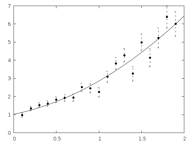
Fig. 31 Weighted fit example with error bars
Regularized Linear Regression Example 1
The next program demonstrates the difference between ordinary and
regularized least squares when the design matrix is near-singular.
In this program, we generate two random normally distributed variables
 and
and  , with
  so that
and are nearly colinear. We then set a third dependent
variable
so that
and are nearly colinear. We then set a third dependent
variable  and solve for the coefficients
 of the model
  .
Since
.
Since  , the design matrix is nearly
singular, leading to unstable ordinary least squares solutions.
, the design matrix is nearly
singular, leading to unstable ordinary least squares solutions.
Here is the program output:
matrix condition number = 1.025113e+04

=== Unregularized fit ===
best fit: y = -43.6588 u + 45.6636 v
residual norm = 31.6248
solution norm = 63.1764
chisq/dof = 1.00213

=== Regularized fit (L-curve) ===
optimal lambda: 4.51103
best fit: y = 1.00113 u + 1.0032 v
residual norm = 31.6547
solution norm = 1.41728
chisq/dof = 1.04499

=== Regularized fit (GCV) ===
optimal lambda: 0.0232029
best fit: y = -19.8367 u + 21.8417 v
residual norm = 31.6332
solution norm = 29.5051
chisq/dof = 1.00314
We see that the ordinary least squares solution is completely wrong,
while the L-curve regularized method with the optimal
 finds the correct solution
 . The GCV regularized method finds
a regularization parameter
. The GCV regularized method finds
a regularization parameter  which is too
small to give an accurate solution, although it performs better than OLS.
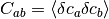
The L-curve and its computed corner, as well as the GCV curve and its
minimum are plotted in Fig. 32.
which is too
small to give an accurate solution, although it performs better than OLS.
The L-curve and its computed corner, as well as the GCV curve and its
minimum are plotted in Fig. 32.
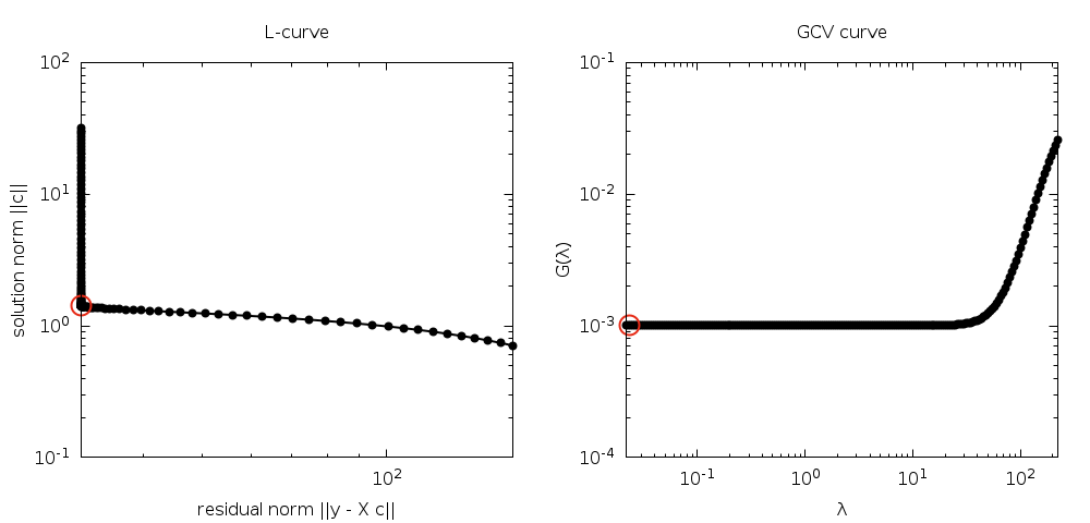
Fig. 32 L-curve and GCV curve for example program.
The program is given below.
#include <gsl/gsl_math.h>
#include <gsl/gsl_vector.h>
#include <gsl/gsl_matrix.h>
#include <gsl/gsl_rng.h>
#include <gsl/gsl_randist.h>
#include <gsl/gsl_multifit.h>
int
main()
{
const size_t n = 1000; /* number of observations */
const size_t p = 2; /* number of model parameters */
size_t i;
gsl_rng *r = gsl_rng_alloc(gsl_rng_default);
gsl_matrix *X = gsl_matrix_alloc(n, p);
gsl_vector *y = gsl_vector_alloc(n);
for (i = 0; i < n; ++i)
{
/* generate first random variable u */
double ui = 5.0 * gsl_ran_gaussian(r, 1.0);
/* set v = u + noise */
double vi = ui + gsl_ran_gaussian(r, 0.001);
/* set y = u + v + noise */
double yi = ui + vi + gsl_ran_gaussian(r, 1.0);
/* since u =~ v, the matrix X is ill-conditioned */
gsl_matrix_set(X, i, 0, ui);
gsl_matrix_set(X, i, 1, vi);
/* rhs vector */
gsl_vector_set(y, i, yi);
}
{
const size_t npoints = 200; /* number of points on L-curve and GCV curve */
gsl_multifit_linear_workspace *w =
gsl_multifit_linear_alloc(n, p);
gsl_vector *c = gsl_vector_alloc(p); /* OLS solution */
gsl_vector *c_lcurve = gsl_vector_alloc(p); /* regularized solution (L-curve) */
gsl_vector *c_gcv = gsl_vector_alloc(p); /* regularized solution (GCV) */
gsl_vector *reg_param = gsl_vector_alloc(npoints);
gsl_vector *rho = gsl_vector_alloc(npoints); /* residual norms */
gsl_vector *eta = gsl_vector_alloc(npoints); /* solution norms */
gsl_vector *G = gsl_vector_alloc(npoints); /* GCV function values */
double lambda_l; /* optimal regularization parameter (L-curve) */
double lambda_gcv; /* optimal regularization parameter (GCV) */
double G_gcv; /* G(lambda_gcv) */
size_t reg_idx; /* index of optimal lambda */
double rcond; /* reciprocal condition number of X */
double chisq, rnorm, snorm;
/* compute SVD of X */
gsl_multifit_linear_svd(X, w);
rcond = gsl_multifit_linear_rcond(w);
fprintf(stderr, "matrix condition number = %e\n\n", 1.0 / rcond);
/* unregularized (standard) least squares fit, lambda = 0 */
gsl_multifit_linear_solve(0.0, X, y, c, &rnorm, &snorm, w);
chisq = pow(rnorm, 2.0);
fprintf(stderr, "=== Unregularized fit ===\n");
fprintf(stderr, "best fit: y = %g u + %g v\n",
gsl_vector_get(c, 0), gsl_vector_get(c, 1));
fprintf(stderr, "residual norm = %g\n", rnorm);
fprintf(stderr, "solution norm = %g\n", snorm);
fprintf(stderr, "chisq/dof = %g\n", chisq / (n - p));
/* calculate L-curve and find its corner */
gsl_multifit_linear_lcurve(y, reg_param, rho, eta, w);
gsl_multifit_linear_lcorner(rho, eta, ®_idx);
/* store optimal regularization parameter */
lambda_l = gsl_vector_get(reg_param, reg_idx);
/* regularize with lambda_l */
gsl_multifit_linear_solve(lambda_l, X, y, c_lcurve, &rnorm, &snorm, w);
chisq = pow(rnorm, 2.0) + pow(lambda_l * snorm, 2.0);
fprintf(stderr, "\n=== Regularized fit (L-curve) ===\n");
fprintf(stderr, "optimal lambda: %g\n", lambda_l);
fprintf(stderr, "best fit: y = %g u + %g v\n",
gsl_vector_get(c_lcurve, 0), gsl_vector_get(c_lcurve, 1));
fprintf(stderr, "residual norm = %g\n", rnorm);
fprintf(stderr, "solution norm = %g\n", snorm);
fprintf(stderr, "chisq/dof = %g\n", chisq / (n - p));
/* calculate GCV curve and find its minimum */
gsl_multifit_linear_gcv(y, reg_param, G, &lambda_gcv, &G_gcv, w);
/* regularize with lambda_gcv */
gsl_multifit_linear_solve(lambda_gcv, X, y, c_gcv, &rnorm, &snorm, w);
chisq = pow(rnorm, 2.0) + pow(lambda_gcv * snorm, 2.0);
fprintf(stderr, "\n=== Regularized fit (GCV) ===\n");
fprintf(stderr, "optimal lambda: %g\n", lambda_gcv);
fprintf(stderr, "best fit: y = %g u + %g v\n",
gsl_vector_get(c_gcv, 0), gsl_vector_get(c_gcv, 1));
fprintf(stderr, "residual norm = %g\n", rnorm);
fprintf(stderr, "solution norm = %g\n", snorm);
fprintf(stderr, "chisq/dof = %g\n", chisq / (n - p));
/* output L-curve and GCV curve */
for (i = 0; i < npoints; ++i)
{
printf("%e %e %e %e\n",
gsl_vector_get(reg_param, i),
gsl_vector_get(rho, i),
gsl_vector_get(eta, i),
gsl_vector_get(G, i));
}
/* output L-curve corner point */
printf("\n\n%f %f\n",
gsl_vector_get(rho, reg_idx),
gsl_vector_get(eta, reg_idx));
/* output GCV curve corner minimum */
printf("\n\n%e %e\n",
lambda_gcv,
G_gcv);
gsl_multifit_linear_free(w);
gsl_vector_free(c);
gsl_vector_free(c_lcurve);
gsl_vector_free(reg_param);
gsl_vector_free(rho);
gsl_vector_free(eta);
gsl_vector_free(G);
}
gsl_rng_free(r);
gsl_matrix_free(X);
gsl_vector_free(y);
return 0;
}
Regularized Linear Regression Example 2
The following example program minimizes the cost function
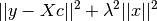
where is the  -by-
-by- Hilbert matrix whose
entries are given by
Hilbert matrix whose
entries are given by
and the right hand side vector is given by
![y = [1,-1,1,-1,1,-1,1,-1,1,-1]^T](_images/math/aec485cb5570fc30b08e31e4d2390af58f0d8b97.png) . Solutions
are computed for
. Solutions
are computed for  (unregularized) as
well as for optimal parameters chosen by
analyzing the L-curve and GCV curve.
(unregularized) as
well as for optimal parameters chosen by
analyzing the L-curve and GCV curve.
Here is the program output:
matrix condition number = 3.565872e+09

=== Unregularized fit ===
residual norm = 2.15376
solution norm = 2.92217e+09
chisq/dof = 2.31934

=== Regularized fit (L-curve) ===
optimal lambda: 7.11407e-07
residual norm = 2.60386
solution norm = 424507
chisq/dof = 3.43565

=== Regularized fit (GCV) ===
optimal lambda: 1.72278
residual norm = 3.1375
solution norm = 0.139357
chisq/dof = 4.95076
Here we see the unregularized solution results in a large solution
norm due to the ill-conditioned matrix. The L-curve solution finds
a small value of  which still results in
a badly conditioned system and a large solution norm. The GCV method
finds a parameter
which still results in
a badly conditioned system and a large solution norm. The GCV method
finds a parameter  which results in a well-conditioned
system and small solution norm.
which results in a well-conditioned
system and small solution norm.
The L-curve and its computed corner, as well as the GCV curve and its minimum are plotted in Fig. 33.
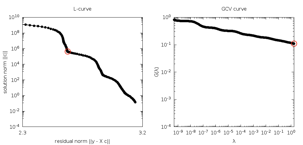
Fig. 33 L-curve and GCV curve for example program.
The program is given below.
#include <gsl/gsl_math.h>
#include <gsl/gsl_vector.h>
#include <gsl/gsl_matrix.h>
#include <gsl/gsl_multifit.h>
#include <gsl/gsl_blas.h>
static int
hilbert_matrix(gsl_matrix * m)
{
const size_t N = m->size1;
const size_t M = m->size2;
size_t i, j;
for (i = 0; i < N; i++)
{
for (j = 0; j < M; j++)
{
gsl_matrix_set(m, i, j, 1.0/(i+j+1.0));
}
}
return GSL_SUCCESS;
}
int
main()
{
const size_t n = 10; /* number of observations */
const size_t p = 8; /* number of model parameters */
size_t i;
gsl_matrix *X = gsl_matrix_alloc(n, p);
gsl_vector *y = gsl_vector_alloc(n);
/* construct Hilbert matrix and rhs vector */
hilbert_matrix(X);
{
double val = 1.0;
for (i = 0; i < n; ++i)
{
gsl_vector_set(y, i, val);
val *= -1.0;
}
}
{
const size_t npoints = 200; /* number of points on L-curve and GCV curve */
gsl_multifit_linear_workspace *w =
gsl_multifit_linear_alloc(n, p);
gsl_vector *c = gsl_vector_alloc(p); /* OLS solution */
gsl_vector *c_lcurve = gsl_vector_alloc(p); /* regularized solution (L-curve) */
gsl_vector *c_gcv = gsl_vector_alloc(p); /* regularized solution (GCV) */
gsl_vector *reg_param = gsl_vector_alloc(npoints);
gsl_vector *rho = gsl_vector_alloc(npoints); /* residual norms */
gsl_vector *eta = gsl_vector_alloc(npoints); /* solution norms */
gsl_vector *G = gsl_vector_alloc(npoints); /* GCV function values */
double lambda_l; /* optimal regularization parameter (L-curve) */
double lambda_gcv; /* optimal regularization parameter (GCV) */
double G_gcv; /* G(lambda_gcv) */
size_t reg_idx; /* index of optimal lambda */
double rcond; /* reciprocal condition number of X */
double chisq, rnorm, snorm;
/* compute SVD of X */
gsl_multifit_linear_svd(X, w);
rcond = gsl_multifit_linear_rcond(w);
fprintf(stderr, "matrix condition number = %e\n", 1.0 / rcond);
/* unregularized (standard) least squares fit, lambda = 0 */
gsl_multifit_linear_solve(0.0, X, y, c, &rnorm, &snorm, w);
chisq = pow(rnorm, 2.0);
fprintf(stderr, "\n=== Unregularized fit ===\n");
fprintf(stderr, "residual norm = %g\n", rnorm);
fprintf(stderr, "solution norm = %g\n", snorm);
fprintf(stderr, "chisq/dof = %g\n", chisq / (n - p));
/* calculate L-curve and find its corner */
gsl_multifit_linear_lcurve(y, reg_param, rho, eta, w);
gsl_multifit_linear_lcorner(rho, eta, ®_idx);
/* store optimal regularization parameter */
lambda_l = gsl_vector_get(reg_param, reg_idx);
/* regularize with lambda_l */
gsl_multifit_linear_solve(lambda_l, X, y, c_lcurve, &rnorm, &snorm, w);
chisq = pow(rnorm, 2.0) + pow(lambda_l * snorm, 2.0);
fprintf(stderr, "\n=== Regularized fit (L-curve) ===\n");
fprintf(stderr, "optimal lambda: %g\n", lambda_l);
fprintf(stderr, "residual norm = %g\n", rnorm);
fprintf(stderr, "solution norm = %g\n", snorm);
fprintf(stderr, "chisq/dof = %g\n", chisq / (n - p));
/* calculate GCV curve and find its minimum */
gsl_multifit_linear_gcv(y, reg_param, G, &lambda_gcv, &G_gcv, w);
/* regularize with lambda_gcv */
gsl_multifit_linear_solve(lambda_gcv, X, y, c_gcv, &rnorm, &snorm, w);
chisq = pow(rnorm, 2.0) + pow(lambda_gcv * snorm, 2.0);
fprintf(stderr, "\n=== Regularized fit (GCV) ===\n");
fprintf(stderr, "optimal lambda: %g\n", lambda_gcv);
fprintf(stderr, "residual norm = %g\n", rnorm);
fprintf(stderr, "solution norm = %g\n", snorm);
fprintf(stderr, "chisq/dof = %g\n", chisq / (n - p));
/* output L-curve and GCV curve */
for (i = 0; i < npoints; ++i)
{
printf("%e %e %e %e\n",
gsl_vector_get(reg_param, i),
gsl_vector_get(rho, i),
gsl_vector_get(eta, i),
gsl_vector_get(G, i));
}
/* output L-curve corner point */
printf("\n\n%f %f\n",
gsl_vector_get(rho, reg_idx),
gsl_vector_get(eta, reg_idx));
/* output GCV curve corner minimum */
printf("\n\n%e %e\n",
lambda_gcv,
G_gcv);
gsl_multifit_linear_free(w);
gsl_vector_free(c);
gsl_vector_free(c_lcurve);
gsl_vector_free(reg_param);
gsl_vector_free(rho);
gsl_vector_free(eta);
gsl_vector_free(G);
}
gsl_matrix_free(X);
gsl_vector_free(y);
return 0;
}
Robust Linear Regression Example
The next program demonstrates the advantage of robust least squares on
a dataset with outliers. The program generates linear  data pairs on the line
  , adds some random
noise, and inserts 3 outliers into the dataset. Both the robust
and ordinary least squares (OLS) coefficients are computed for
comparison.
, adds some random
noise, and inserts 3 outliers into the dataset. Both the robust
and ordinary least squares (OLS) coefficients are computed for
comparison.
#include <stdio.h>
#include <gsl/gsl_multifit.h>
#include <gsl/gsl_randist.h>

int
dofit(const gsl_multifit_robust_type *T,
      const gsl_matrix *X, const gsl_vector *y,
      gsl_vector *c, gsl_matrix *cov)
{
  int s;
  gsl_multifit_robust_workspace * work
    = gsl_multifit_robust_alloc (T, X->size1, X->size2);

  s = gsl_multifit_robust (X, y, c, cov, work);
  gsl_multifit_robust_free (work);

  return s;
}

int
main (int argc, char **argv)
{
  size_t i;
  size_t n;
  const size_t p = 2; /* linear fit */
  gsl_matrix *X, *cov;
  gsl_vector *x, *y, *c, *c_ols;
  const double a = 1.45; /* slope */
  const double b = 3.88; /* intercept */
  gsl_rng *r;

  if (argc != 2)
    {
      fprintf (stderr,"usage: robfit n\n");
      exit (-1);
    }

  n = atoi (argv[1]);

  X = gsl_matrix_alloc (n, p);
  x = gsl_vector_alloc (n);
  y = gsl_vector_alloc (n);

  c = gsl_vector_alloc (p);
  c_ols = gsl_vector_alloc (p);
  cov = gsl_matrix_alloc (p, p);

  r = gsl_rng_alloc(gsl_rng_default);

  /* generate linear dataset */
  for (i = 0; i < n - 3; i++)
    {
      double dx = 10.0 / (n - 1.0);
      double ei = gsl_rng_uniform(r);
      double xi = -5.0 + i * dx;
      double yi = a * xi + b;

      gsl_vector_set (x, i, xi);
      gsl_vector_set (y, i, yi + ei);
    }

  /* add a few outliers */
  gsl_vector_set(x, n - 3, 4.7);
  gsl_vector_set(y, n - 3, -8.3);

  gsl_vector_set(x, n - 2, 3.5);
  gsl_vector_set(y, n - 2, -6.7);

  gsl_vector_set(x, n - 1, 4.1);
  gsl_vector_set(y, n - 1, -6.0);

  /* construct design matrix X for linear fit */
  for (i = 0; i < n; ++i)
    {
      double xi = gsl_vector_get(x, i);

      gsl_matrix_set (X, i, 0, 1.0);
      gsl_matrix_set (X, i, 1, xi);
    }

  /* perform robust and OLS fit */
  dofit(gsl_multifit_robust_ols, X, y, c_ols, cov);
  dofit(gsl_multifit_robust_bisquare, X, y, c, cov);

  /* output data and model */
  for (i = 0; i < n; ++i)
    {
      double xi = gsl_vector_get(x, i);
      double yi = gsl_vector_get(y, i);
      gsl_vector_view v = gsl_matrix_row(X, i);
      double y_ols, y_rob, y_err;

      gsl_multifit_robust_est(&v.vector, c, cov, &y_rob, &y_err);
      gsl_multifit_robust_est(&v.vector, c_ols, cov, &y_ols, &y_err);

      printf("%g %g %g %g\n", xi, yi, y_rob, y_ols);
    }

#define C(i) (gsl_vector_get(c,(i)))
#define COV(i,j) (gsl_matrix_get(cov,(i),(j)))

  {
    printf ("# best fit: Y = %g + %g X\n",
            C(0), C(1));

    printf ("# covariance matrix:\n");
    printf ("# [ %+.5e, %+.5e\n",
               COV(0,0), COV(0,1));
    printf ("#   %+.5e, %+.5e\n",
               COV(1,0), COV(1,1));
  }

  gsl_matrix_free (X);
  gsl_vector_free (x);
  gsl_vector_free (y);
  gsl_vector_free (c);
  gsl_vector_free (c_ols);
  gsl_matrix_free (cov);
  gsl_rng_free(r);

  return 0;
}
The output from the program is shown in Fig. 34.
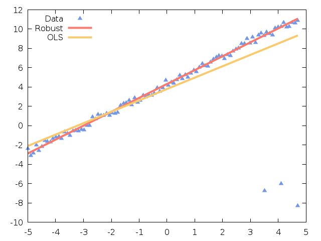
Fig. 34 Linear fit to dataset with outliers.
Large Dense Linear Regression Example
The following program demostrates the large dense linear least squares
solvers. This example is adapted from Trefethen and Bau,
and fits the function 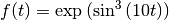 on
the interval
on
the interval ![[0,1]](_images/math/e7e8ac4ddd4ab0fc62c2a6435f8373f48c776858.png) with a degree 15 polynomial. The
program generates
with a degree 15 polynomial. The
program generates  equally spaced points
 on this interval, calculates the function value
and adds random noise to determine the observation value
. The entries of the least squares matrix are
on this interval, calculates the function value
and adds random noise to determine the observation value
. The entries of the least squares matrix are
 , representing a polynomial fit. The
matrix is highly ill-conditioned, with a condition number
of about
, representing a polynomial fit. The
matrix is highly ill-conditioned, with a condition number
of about  . The program accumulates the
matrix into the least squares system in 5 blocks, each with
10000 rows. This way the full matrix is never
stored in memory. We solve the system with both the
normal equations and TSQR methods. The results are shown
in Fig. 35. In the top left plot, the TSQR
solution provides a reasonable agreement to the exact solution,
while the normal equations method fails completely since the
Cholesky factorization fails due to the ill-conditioning of the matrix.
In the bottom left plot, we show the L-curve calculated from TSQR, which exhibits multiple corners.
In the top right panel, we plot a regularized solution using
. The program accumulates the
matrix into the least squares system in 5 blocks, each with
10000 rows. This way the full matrix is never
stored in memory. We solve the system with both the
normal equations and TSQR methods. The results are shown
in Fig. 35. In the top left plot, the TSQR
solution provides a reasonable agreement to the exact solution,
while the normal equations method fails completely since the
Cholesky factorization fails due to the ill-conditioning of the matrix.
In the bottom left plot, we show the L-curve calculated from TSQR, which exhibits multiple corners.
In the top right panel, we plot a regularized solution using
 . The TSQR and normal solutions now agree,
however they are unable to provide a good fit due to the damping.
This indicates that for some ill-conditioned
problems, regularizing the normal equations does not improve the
solution. This is further illustrated in the bottom right panel,
where we plot the L-curve calculated from the normal equations.
The curve agrees with the TSQR curve for larger damping parameters,
but for small , the normal equations approach cannot
provide accurate solution vectors leading to numerical
inaccuracies in the left portion of the curve.
. The TSQR and normal solutions now agree,
however they are unable to provide a good fit due to the damping.
This indicates that for some ill-conditioned
problems, regularizing the normal equations does not improve the
solution. This is further illustrated in the bottom right panel,
where we plot the L-curve calculated from the normal equations.
The curve agrees with the TSQR curve for larger damping parameters,
but for small , the normal equations approach cannot
provide accurate solution vectors leading to numerical
inaccuracies in the left portion of the curve.
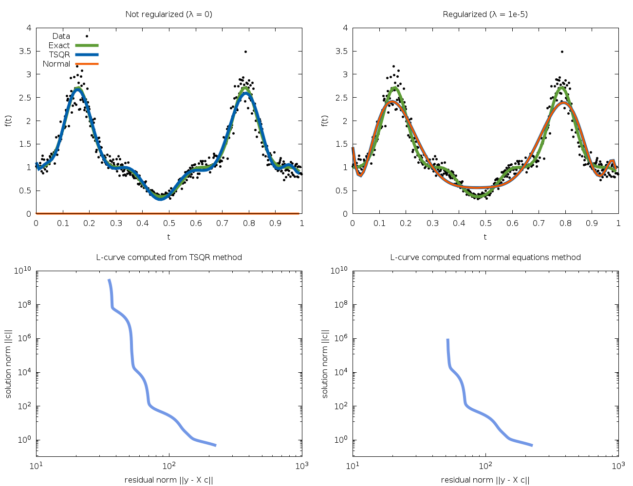
Fig. 35 Top left: unregularized solutions; top right: regularized solutions; bottom left: L-curve for TSQR method; bottom right: L-curve from normal equations method.
#include <gsl/gsl_math.h>
#include <gsl/gsl_vector.h>
#include <gsl/gsl_matrix.h>
#include <gsl/gsl_rng.h>
#include <gsl/gsl_randist.h>
#include <gsl/gsl_multifit.h>
#include <gsl/gsl_multilarge.h>
#include <gsl/gsl_blas.h>
#include <gsl/gsl_errno.h>

/* function to be fitted */
double
func(const double t)
{
  double x = sin(10.0 * t);
  return exp(x*x*x);
}

/* construct a row of the least squares matrix */
int
build_row(const double t, gsl_vector *row)
{
  const size_t p = row->size;
  double Xj = 1.0;
  size_t j;

  for (j = 0; j < p; ++j)
    {
      gsl_vector_set(row, j, Xj);
      Xj *= t;
    }

  return 0;
}

int
solve_system(const int print_data, const gsl_multilarge_linear_type * T,
             const double lambda, const size_t n, const size_t p,
             gsl_vector * c)
{
  const size_t nblock = 5;         /* number of blocks to accumulate */
  const size_t nrows = n / nblock; /* number of rows per block */
  gsl_multilarge_linear_workspace * w =
    gsl_multilarge_linear_alloc(T, p);
  gsl_matrix *X = gsl_matrix_alloc(nrows, p);
  gsl_vector *y = gsl_vector_alloc(nrows);
  gsl_rng *r = gsl_rng_alloc(gsl_rng_default);
  const size_t nlcurve = 200;
  gsl_vector *reg_param = gsl_vector_alloc(nlcurve);
  gsl_vector *rho = gsl_vector_calloc(nlcurve);
  gsl_vector *eta = gsl_vector_calloc(nlcurve);
  size_t rowidx = 0;
  double rnorm, snorm, rcond;
  double t = 0.0;
  double dt = 1.0 / (n - 1.0);

  while (rowidx < n)
    {
      size_t nleft = n - rowidx;         /* number of rows left to accumulate */
      size_t nr = GSL_MIN(nrows, nleft); /* number of rows in this block */
      gsl_matrix_view Xv = gsl_matrix_submatrix(X, 0, 0, nr, p);
      gsl_vector_view yv = gsl_vector_subvector(y, 0, nr);
      size_t i;

      /* build (X,y) block with 'nr' rows */
      for (i = 0; i < nr; ++i)
        {
          gsl_vector_view row = gsl_matrix_row(&Xv.matrix, i);
          double fi = func(t);
          double ei = gsl_ran_gaussian (r, 0.1 * fi); /* noise */
          double yi = fi + ei;

          /* construct this row of LS matrix */
          build_row(t, &row.vector);

          /* set right hand side value with added noise */
          gsl_vector_set(&yv.vector, i, yi);

          if (print_data && (i % 100 == 0))
            printf("%f %f\n", t, yi);

          t += dt;
        }

      /* accumulate (X,y) block into LS system */
      gsl_multilarge_linear_accumulate(&Xv.matrix, &yv.vector, w);

      rowidx += nr;
    }

  if (print_data)
    printf("\n\n");

  /* compute L-curve */
  gsl_multilarge_linear_lcurve(reg_param, rho, eta, w);

  /* solve large LS system and store solution in c */
  gsl_multilarge_linear_solve(lambda, c, &rnorm, &snorm, w);

  /* compute reciprocal condition number */
  gsl_multilarge_linear_rcond(&rcond, w);

  fprintf(stderr, "=== Method %s ===\n", gsl_multilarge_linear_name(w));
  fprintf(stderr, "condition number = %e\n", 1.0 / rcond);
  fprintf(stderr, "residual norm    = %e\n", rnorm);
  fprintf(stderr, "solution norm    = %e\n", snorm);

  /* output L-curve */
  {
    size_t i;
    for (i = 0; i < nlcurve; ++i)
      {
        printf("%.12e %.12e %.12e\n",
               gsl_vector_get(reg_param, i),
               gsl_vector_get(rho, i),
               gsl_vector_get(eta, i));
      }
    printf("\n\n");
  }

  gsl_matrix_free(X);
  gsl_vector_free(y);
  gsl_multilarge_linear_free(w);
  gsl_rng_free(r);
  gsl_vector_free(reg_param);
  gsl_vector_free(rho);
  gsl_vector_free(eta);

  return 0;
}

int
main(int argc, char *argv[])
{
  const size_t n = 50000;   /* number of observations */
  const size_t p = 16;      /* polynomial order + 1 */
  double lambda = 0.0;      /* regularization parameter */
  gsl_vector *c_tsqr = gsl_vector_calloc(p);
  gsl_vector *c_normal = gsl_vector_calloc(p);

  if (argc > 1)
    lambda = atof(argv[1]);

  /* turn off error handler so normal equations method won't abort */
  gsl_set_error_handler_off();

  /* solve system with TSQR method */
  solve_system(1, gsl_multilarge_linear_tsqr, lambda, n, p, c_tsqr);

  /* solve system with Normal equations method */
  solve_system(0, gsl_multilarge_linear_normal, lambda, n, p, c_normal);

  /* output solutions */
  {
    gsl_vector *v = gsl_vector_alloc(p);
    double t;

    for (t = 0.0; t <= 1.0; t += 0.01)
      {
        double f_exact = func(t);
        double f_tsqr, f_normal;

        build_row(t, v);
        gsl_blas_ddot(v, c_tsqr, &f_tsqr);
        gsl_blas_ddot(v, c_normal, &f_normal);

        printf("%f %e %e %e\n", t, f_exact, f_tsqr, f_normal);
      }

    gsl_vector_free(v);
  }

  gsl_vector_free(c_tsqr);
  gsl_vector_free(c_normal);

  return 0;
}
References and Further Reading
A summary of formulas and techniques for least squares fitting can be found in the “Statistics” chapter of the Annual Review of Particle Physics prepared by the Particle Data Group,
Review of Particle Properties, R.M. Barnett et al., Physical Review D54, 1 (1996) http://pdg.lbl.gov
The Review of Particle Physics is available online at the website given above.
The tests used to prepare these routines are based on the NIST Statistical Reference Datasets. The datasets and their documentation are available from NIST at the following website,
http://www.nist.gov/itl/div898/strd/index.html
More information on Tikhonov regularization can be found in
Hansen, P. C. (1998), Rank-Deficient and Discrete Ill-Posed Problems: Numerical Aspects of Linear Inversion. SIAM Monogr. on Mathematical Modeling and Computation, Society for Industrial and Applied Mathematics
M. Rezghi and S. M. Hosseini (2009), A new variant of L-curve for Tikhonov regularization, Journal of Computational and Applied Mathematics, Volume 231, Issue 2, pages 914-924.
The GSL implementation of robust linear regression closely follows the publications
DuMouchel, W. and F. O’Brien (1989), “Integrating a robust option into a multiple regression computing environment,” Computer Science and Statistics: Proceedings of the 21st Symposium on the Interface, American Statistical Association
Street, J.O., R.J. Carroll, and D. Ruppert (1988), “A note on computing robust regression estimates via iteratively reweighted least squares,” The American Statistician, v. 42, pp. 152-154.
More information about the normal equations and TSQR approach for solving large linear least squares systems can be found in the publications
Trefethen, L. N. and Bau, D. (1997), “Numerical Linear Algebra”, SIAM.
Demmel, J., Grigori, L., Hoemmen, M. F., and Langou, J. “Communication-optimal parallel and sequential QR and LU factorizations”, UCB Technical Report No. UCB/EECS-2008-89, 2008.