Nonlinear Least-Squares Fitting
This chapter describes functions for multidimensional nonlinear least-squares fitting. There are generally two classes of algorithms for solving nonlinear least squares problems, which fall under line search methods and trust region methods. GSL currently implements only trust region methods and provides the user with full access to intermediate steps of the iteration. The user also has the ability to tune a number of parameters which affect low-level aspects of the algorithm which can help to accelerate convergence for the specific problem at hand. GSL provides two separate interfaces for nonlinear least squares fitting. The first is designed for small to moderate sized problems, and the second is designed for very large problems, which may or may not have significant sparse structure.
The header file gsl_multifit_nlinear.h contains prototypes for the
multidimensional nonlinear fitting functions and related declarations
relating to the small to moderate sized systems.
The header file gsl_multilarge_nlinear.h contains prototypes for the
multidimensional nonlinear fitting functions and related declarations
relating to large systems.
Overview
The problem of multidimensional nonlinear least-squares fitting requires
the minimization of the squared residuals of  functions,
 , in
, in  parameters,
  ,
,
In trust region methods, the objective (or cost) function  is approximated
by a model function
is approximated
by a model function  in the vicinity of some point
  . The
model function is often simply a second order Taylor series expansion around the
point , ie:
. The
model function is often simply a second order Taylor series expansion around the
point , ie:
where  is the gradient vector at the point ,
 is the Hessian matrix at , or some
approximation to it, and
is the Hessian matrix at , or some
approximation to it, and  is the -by- Jacobian matrix
In order to find the next step  , we minimize the model function
, but search for solutions only within a region where
we trust that is a good approximation to the objective
function
, we minimize the model function
, but search for solutions only within a region where
we trust that is a good approximation to the objective
function  . In other words,
we seek a solution of the trust region subproblem (TRS)
. In other words,
we seek a solution of the trust region subproblem (TRS)

where  is the trust region radius and
  is
a scaling matrix. If
is
a scaling matrix. If  , then the trust region is a ball
of radius
, then the trust region is a ball
of radius  centered at . In some applications,
the parameter vector
centered at . In some applications,
the parameter vector  may have widely different scales. For
example, one parameter might be a temperature on the order of
may have widely different scales. For
example, one parameter might be a temperature on the order of
 K, while another might be a length on the order of
 m. In such cases, a spherical trust region may not
be the best choice, since if
m. In such cases, a spherical trust region may not
be the best choice, since if  changes rapidly along
directions with one scale, and more slowly along directions with
a different scale, the model function
changes rapidly along
directions with one scale, and more slowly along directions with
a different scale, the model function  may be a poor
approximation to along the rapidly changing directions.
In such problems, it may be best to use an elliptical trust region,
by setting to a diagonal matrix whose entries are designed
so that the scaled step
may be a poor
approximation to along the rapidly changing directions.
In such problems, it may be best to use an elliptical trust region,
by setting to a diagonal matrix whose entries are designed
so that the scaled step  has entries of approximately the same
order of magnitude.
has entries of approximately the same
order of magnitude.
The trust region subproblem above normally amounts to solving a
linear least squares system (or multiple systems) for the step
. Once is computed, it is checked whether
or not it reduces the objective function . A useful
statistic for this is to look at the ratio
where the numerator is the actual reduction of the objective function
due to the step  , and the denominator is the predicted
reduction due to the model . If
, and the denominator is the predicted
reduction due to the model . If  is negative,
it means that the step increased the objective function
and so it is rejected. If is positive,
then we have found a step which reduced the objective function and
it is accepted. Furthermore, if is close to 1,
then this indicates that the model function is a good approximation
to the objective function in the trust region, and so on the next
iteration the trust region is enlarged in order to take more ambitious
steps. When a step is rejected, the trust region is made smaller and
the TRS is solved again. An outline for the general trust region method
used by GSL can now be given.
is negative,
it means that the step increased the objective function
and so it is rejected. If is positive,
then we have found a step which reduced the objective function and
it is accepted. Furthermore, if is close to 1,
then this indicates that the model function is a good approximation
to the objective function in the trust region, and so on the next
iteration the trust region is enlarged in order to take more ambitious
steps. When a step is rejected, the trust region is made smaller and
the TRS is solved again. An outline for the general trust region method
used by GSL can now be given.
Trust Region Algorithm
Initialize: given
 , construct
  ,
,  and
and 
For k = 0, 1, 2, …
If converged, then stop
Solve TRS for trial step
Evaluate trial step by computing
- 1). if step is accepted, set
 and increase radius,
- 2). if step is rejected, set
 and decrease radius,
  ; goto 2(b)
- 1). if step is accepted, set
Construct
 and
and 
GSL offers the user a number of different algorithms for solving the trust
region subproblem in 2(b), as well as different choices of scaling matrices
and different methods of updating the trust region radius
. Therefore, while reasonable default methods are provided,
the user has a lot of control to fine-tune the various steps of the
algorithm for their specific problem.
Solving the Trust Region Subproblem (TRS)
Below we describe the methods available for solving the trust region
subproblem. The methods available provide either exact or approximate
solutions to the trust region subproblem. In all algorithms below,
the Hessian matrix  is approximated as
  ,
where
,
where  . In all methods, the solution of the TRS
involves solving a linear least squares system involving the Jacobian
matrix. For small to moderate sized problems (
. In all methods, the solution of the TRS
involves solving a linear least squares system involving the Jacobian
matrix. For small to moderate sized problems (gsl_multifit_nlinear interface),
this is accomplished by factoring the full Jacobian matrix, which is provided
by the user, with the Cholesky, QR, or SVD decompositions. For large systems
(gsl_multilarge_nlinear interface), the user has two choices. One
is to solve the system iteratively, without needing to store the full
Jacobian matrix in memory. With this method, the user must provide a routine
to calculate the matrix-vector products  or
or  for a given vector
  .
This iterative method is particularly useful for systems where the Jacobian has
sparse structure, since forming matrix-vector products can be done cheaply. The
second option for large systems involves forming the normal equations matrix
.
This iterative method is particularly useful for systems where the Jacobian has
sparse structure, since forming matrix-vector products can be done cheaply. The
second option for large systems involves forming the normal equations matrix
 and then factoring it using a Cholesky decomposition. The normal
equations matrix is -by-, typically much smaller than the full
-by- Jacobian, and can usually be stored in memory even if the full
Jacobian matrix cannot. This option is useful for large, dense systems, or if the
iterative method has difficulty converging.
and then factoring it using a Cholesky decomposition. The normal
equations matrix is -by-, typically much smaller than the full
-by- Jacobian, and can usually be stored in memory even if the full
Jacobian matrix cannot. This option is useful for large, dense systems, or if the
iterative method has difficulty converging.
Levenberg-Marquardt
There is a theorem which states that if is a solution
to the trust region subproblem given above, then there exists
 such that
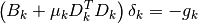
with  . This
forms the basis of the Levenberg-Marquardt algorithm, which controls
the trust region size by adjusting the parameter
. This
forms the basis of the Levenberg-Marquardt algorithm, which controls
the trust region size by adjusting the parameter  rather than the radius directly. For each radius
, there is a unique parameter which
solves the TRS, and they have an inverse relationship, so that large values of
correspond to smaller trust regions, while small
values of correspond to larger trust regions.
rather than the radius directly. For each radius
, there is a unique parameter which
solves the TRS, and they have an inverse relationship, so that large values of
correspond to smaller trust regions, while small
values of correspond to larger trust regions.
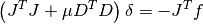
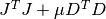
With the approximation , on each iteration,
in order to calculate the step ,
the following linear least squares problem is solved:
![\left[
\begin{array}{c}
J_k \\
\sqrt{\mu_k} D_k
\end{array}
\right]
\delta_k =
-
\left[
\begin{array}{c}
f_k \cr
0
\end{array}
\right]](_images/math/3e54d994a48dc853136043faa932b9f59ef7092a.png)
If the step is accepted, then
is decreased on the next iteration in order
to take a larger step, otherwise it is increased to take
a smaller step. The Levenberg-Marquardt algorithm provides
an exact solution of the trust region subproblem, but
typically has a higher computational cost per iteration
than the approximate methods discussed below, since it
may need to solve the least squares system above several
times for different values of .
Levenberg-Marquardt with Geodesic Acceleration
This method applies a so-called geodesic acceleration correction to
the standard Levenberg-Marquardt step (Transtrum et al, 2011).
By interpreting as a first order step along a geodesic in the
model parameter space (ie: a velocity  ), the geodesic
acceleration
), the geodesic
acceleration  is a second order correction along the
geodesic which is determined by solving the linear least squares system
is a second order correction along the
geodesic which is determined by solving the linear least squares system
![\left[
\begin{array}{c}
J_k \\
\sqrt{\mu_k} D_k
\end{array}
\right]
a_k =
-
\left[
\begin{array}{c}
f_{vv}(x_k) \\
0
\end{array}
\right]](_images/math/6487ffad655f1dbfb0f9e92628d1a174b0294ef1.png)
where  is the second directional derivative of
the residual vector in the velocity direction
is the second directional derivative of
the residual vector in the velocity direction  ,
,
 ,
where
,
where  and
and  are summed over the
parameters. The new total step is then
are summed over the
parameters. The new total step is then  .
The second order correction can be calculated with a modest additional
cost, and has been shown to dramatically reduce the number of iterations
(and expensive Jacobian evaluations) required to reach convergence on a variety
of different problems. In order to utilize the geodesic acceleration, the user must supply a
function which provides the second directional derivative vector
.
The second order correction can be calculated with a modest additional
cost, and has been shown to dramatically reduce the number of iterations
(and expensive Jacobian evaluations) required to reach convergence on a variety
of different problems. In order to utilize the geodesic acceleration, the user must supply a
function which provides the second directional derivative vector
 , or alternatively the library can use a finite
difference method to estimate this vector with one additional function
evaluation of
, or alternatively the library can use a finite
difference method to estimate this vector with one additional function
evaluation of  where
where  is a tunable step size
(see the
is a tunable step size
(see the h_fvv parameter description).
Dogleg
This is Powell’s dogleg method, which finds an approximate solution to the trust region subproblem, by restricting its search to a piecewise linear “dogleg” path, composed of the origin, the Cauchy point which represents the model minimizer along the steepest descent direction, and the Gauss-Newton point, which is the overall minimizer of the unconstrained model. The Gauss-Newton step is calculated by solving

which is the main computational task for each iteration, but only needs to be performed once per iteration. If the Gauss-Newton point is inside the trust region, it is selected as the step. If it is outside, the method then calculates the Cauchy point, which is located along the gradient direction. If the Cauchy point is also outside the trust region, the method assumes that it is still far from the minimum and so proceeds along the gradient direction, truncating the step at the trust region boundary. If the Cauchy point is inside the trust region, with the Gauss-Newton point outside, the method uses a dogleg step, which is a linear combination of the gradient direction and the Gauss-Newton direction, stopping at the trust region boundary.
Double Dogleg
This method is an improvement over the classical dogleg
algorithm, which attempts to include information about
the Gauss-Newton step while the iteration is still far from
the minimum. When the Cauchy point is inside the trust region
and the Gauss-Newton point is outside, the method computes
a scaled Gauss-Newton point and then takes a dogleg step
between the Cauchy point and the scaled Gauss-Newton point.
The scaling is calculated to ensure that the reduction
in the model is about the same as the reduction
provided by the Cauchy point.
Two Dimensional Subspace
The dogleg methods restrict the search for the TRS solution to a 1D curve defined by the Cauchy and Gauss-Newton points. An improvement to this is to search for a solution using the full two dimensional subspace spanned by the Cauchy and Gauss-Newton directions. The dogleg path is of course inside this subspace, and so this method solves the TRS at least as accurately as the dogleg methods. Since this method searches a larger subspace for a solution, it can converge more quickly than dogleg on some problems. Because the subspace is only two dimensional, this method is very efficient and the main computation per iteration is to determine the Gauss-Newton point.
Steihaug-Toint Conjugate Gradient
One difficulty of the dogleg methods is calculating the Gauss-Newton step when the Jacobian matrix is singular. The Steihaug-Toint method also computes a generalized dogleg step, but avoids solving for the Gauss-Newton step directly, instead using an iterative conjugate gradient algorithm. This method performs well at points where the Jacobian is singular, and is also suitable for large-scale problems where factoring the Jacobian matrix could be prohibitively expensive.
Weighted Nonlinear Least-Squares
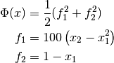
Weighted nonlinear least-squares fitting minimizes the function
where  is the weighting matrix,
and
is the weighting matrix,
and 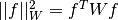 .
The weights
.
The weights  are commonly defined as
  ,
where
,
where  is the error in the
  -th measurement.
A simple change of variables
-th measurement.
A simple change of variables  yields
 , which is in the
same form as the unweighted case. The user can either perform this
transform directly on their function residuals and Jacobian, or use
the
, which is in the
same form as the unweighted case. The user can either perform this
transform directly on their function residuals and Jacobian, or use
the gsl_multifit_nlinear_winit() interface which automatically
performs the correct scaling. To manually perform this transformation,
the residuals and Jacobian should be modified according to
For large systems, the user must perform their own weighting.
Tunable Parameters
The user can tune nearly all aspects of the iteration at allocation
time. For the gsl_multifit_nlinear interface, the user may
modify the gsl_multifit_nlinear_parameters structure, which is
defined as follows:
-
type gsl_multifit_nlinear_parameters
typedef struct
{
  const gsl_multifit_nlinear_trs *trs;        /* trust region subproblem method */
  const gsl_multifit_nlinear_scale *scale;    /* scaling method */
  const gsl_multifit_nlinear_solver *solver;  /* solver method */
  gsl_multifit_nlinear_fdtype fdtype;         /* finite difference method */
  double factor_up;                           /* factor for increasing trust radius */
  double factor_down;                         /* factor for decreasing trust radius */
  double avmax;                               /* max allowed |a|/|v| */
  double h_df;                                /* step size for finite difference Jacobian */
  double h_fvv;                               /* step size for finite difference fvv */
} gsl_multifit_nlinear_parameters;
For the gsl_multilarge_nlinear interface, the user may
modify the gsl_multilarge_nlinear_parameters structure, which is
defined as follows:
-
type gsl_multilarge_nlinear_parameters
typedef struct
{
  const gsl_multilarge_nlinear_trs *trs;       /* trust region subproblem method */
  const gsl_multilarge_nlinear_scale *scale;   /* scaling method */
  const gsl_multilarge_nlinear_solver *solver; /* solver method */
  gsl_multilarge_nlinear_fdtype fdtype;        /* finite difference method */
  double factor_up;                            /* factor for increasing trust radius */
  double factor_down;                          /* factor for decreasing trust radius */
  double avmax;                                /* max allowed |a|/|v| */
  double h_df;                                 /* step size for finite difference Jacobian */
  double h_fvv;                                /* step size for finite difference fvv */
  size_t max_iter;                             /* maximum iterations for trs method */
  double tol;                                  /* tolerance for solving trs */
} gsl_multilarge_nlinear_parameters;
Each of these parameters is discussed in further detail below.
-
type gsl_multifit_nlinear_trs
-
type gsl_multilarge_nlinear_trs
The parameter
trsdetermines the method used to solve the trust region subproblem, and may be selected from the following choices,-
gsl_multifit_nlinear_trs *gsl_multifit_nlinear_trs_lm
-
gsl_multilarge_nlinear_trs *gsl_multilarge_nlinear_trs_lm
This selects the Levenberg-Marquardt algorithm.
-
gsl_multifit_nlinear_trs *gsl_multifit_nlinear_trs_lmaccel
-
gsl_multilarge_nlinear_trs *gsl_multilarge_nlinear_trs_lmaccel
This selects the Levenberg-Marquardt algorithm with geodesic acceleration.
-
gsl_multifit_nlinear_trs *gsl_multifit_nlinear_trs_dogleg
-
gsl_multilarge_nlinear_trs *gsl_multilarge_nlinear_trs_dogleg
This selects the dogleg algorithm.
-
gsl_multifit_nlinear_trs *gsl_multifit_nlinear_trs_ddogleg
-
gsl_multilarge_nlinear_trs *gsl_multilarge_nlinear_trs_ddogleg
This selects the double dogleg algorithm.
-
gsl_multifit_nlinear_trs *gsl_multifit_nlinear_trs_subspace2D
-
gsl_multilarge_nlinear_trs *gsl_multilarge_nlinear_trs_subspace2D
This selects the 2D subspace algorithm.
-
gsl_multilarge_nlinear_trs *gsl_multilarge_nlinear_trs_cgst
This selects the Steihaug-Toint conjugate gradient algorithm. This method is available only for large systems.
-
gsl_multifit_nlinear_trs *gsl_multifit_nlinear_trs_lm
-
type gsl_multifit_nlinear_scale
-
type gsl_multilarge_nlinear_scale
The parameter
scaledetermines the diagonal scaling matrix and
may be selected from the following choices,
and
may be selected from the following choices,-
gsl_multifit_nlinear_scale *gsl_multifit_nlinear_scale_more
-
gsl_multilarge_nlinear_scale *gsl_multilarge_nlinear_scale_more
This damping strategy was suggested by Moré, and corresponds to
 ,
in other words the maximum elements of
,
in other words the maximum elements of
 encountered thus far in the iteration.
This choice of makes the problem scale-invariant,
so that if the model parameters are each scaled
by an arbitrary constant,
encountered thus far in the iteration.
This choice of makes the problem scale-invariant,
so that if the model parameters are each scaled
by an arbitrary constant,  , then
the sequence of iterates produced by the algorithm would
be unchanged. This method can work very well in cases
where the model parameters have widely different scales
(ie: if some parameters are measured in nanometers, while others
are measured in degrees Kelvin). This strategy has been proven
effective on a large class of problems and so it is the library
default, but it may not be the best choice for all problems.
, then
the sequence of iterates produced by the algorithm would
be unchanged. This method can work very well in cases
where the model parameters have widely different scales
(ie: if some parameters are measured in nanometers, while others
are measured in degrees Kelvin). This strategy has been proven
effective on a large class of problems and so it is the library
default, but it may not be the best choice for all problems.
-
gsl_multifit_nlinear_scale *gsl_multifit_nlinear_scale_levenberg
-
gsl_multilarge_nlinear_scale *gsl_multilarge_nlinear_scale_levenberg
This damping strategy was originally suggested by Levenberg, and corresponds to
 . This method has also proven
effective on a large class of problems, but is not scale-invariant.
However, some authors (e.g. Transtrum and Sethna 2012) argue
that this choice is better for problems which are susceptible
to parameter evaporation (ie: parameters go to infinity)
. This method has also proven
effective on a large class of problems, but is not scale-invariant.
However, some authors (e.g. Transtrum and Sethna 2012) argue
that this choice is better for problems which are susceptible
to parameter evaporation (ie: parameters go to infinity)
-
gsl_multifit_nlinear_scale *gsl_multifit_nlinear_scale_marquardt
-
gsl_multilarge_nlinear_scale *gsl_multilarge_nlinear_scale_marquardt
This damping strategy was suggested by Marquardt, and corresponds to
 . This
method is scale-invariant, but it is generally considered
inferior to both the Levenberg and Moré strategies, though
may work well on certain classes of problems.
. This
method is scale-invariant, but it is generally considered
inferior to both the Levenberg and Moré strategies, though
may work well on certain classes of problems.
-
gsl_multifit_nlinear_scale *gsl_multifit_nlinear_scale_more
-
type gsl_multifit_nlinear_solver
-
type gsl_multilarge_nlinear_solver
Solving the trust region subproblem on each iteration almost always requires the solution of the following linear least squares system
![\left[
\begin{array}{c}
J \\
\sqrt{\mu} D
\end{array}
\right]
\delta =
-
\left[
\begin{array}{c}
f \\
0
\end{array}
\right]](_images/math/da00ff066889be51b5261367af0f59fb5255aa9f.png)
The
solverparameter determines how the system is solved and can be selected from the following choices:-
gsl_multifit_nlinear_solver *gsl_multifit_nlinear_solver_qr
This method solves the system using a rank revealing QR decomposition of the Jacobian
. This method will
produce reliable solutions in cases where the Jacobian
is rank deficient or near-singular but does require about
twice as many operations as the Cholesky method discussed
below.
-
gsl_multifit_nlinear_solver *gsl_multifit_nlinear_solver_cholesky
-
gsl_multilarge_nlinear_solver *gsl_multilarge_nlinear_solver_cholesky
This method solves the alternate normal equations problem
by using a Cholesky decomposition of the matrix
 . This method is faster than the
QR approach, however it is susceptible to numerical instabilities
if the Jacobian matrix is rank deficient or near-singular. In
these cases, an attempt is made to reduce the condition number
of the matrix using Jacobi preconditioning, but for highly
ill-conditioned problems the QR approach is better. If it is
known that the Jacobian matrix is well conditioned, this method
is accurate and will perform faster than the QR approach.
. This method is faster than the
QR approach, however it is susceptible to numerical instabilities
if the Jacobian matrix is rank deficient or near-singular. In
these cases, an attempt is made to reduce the condition number
of the matrix using Jacobi preconditioning, but for highly
ill-conditioned problems the QR approach is better. If it is
known that the Jacobian matrix is well conditioned, this method
is accurate and will perform faster than the QR approach.
-
gsl_multifit_nlinear_solver *gsl_multifit_nlinear_solver_mcholesky
-
gsl_multilarge_nlinear_solver *gsl_multilarge_nlinear_solver_mcholesky
This method solves the alternate normal equations problem
by using a modified Cholesky decomposition of the matrix
. This is more suitable for the dogleg
methods where the parameter  , and the matrix
may be ill-conditioned or indefinite causing the standard Cholesky
decomposition to fail. This method is based on Level 2 BLAS
and is thus slower than the standard Cholesky decomposition, which
is based on Level 3 BLAS.
, and the matrix
may be ill-conditioned or indefinite causing the standard Cholesky
decomposition to fail. This method is based on Level 2 BLAS
and is thus slower than the standard Cholesky decomposition, which
is based on Level 3 BLAS.
-
gsl_multifit_nlinear_solver *gsl_multifit_nlinear_solver_svd
This method solves the system using a singular value decomposition of the Jacobian
. This method will
produce the most reliable solutions for ill-conditioned Jacobians
but is also the slowest solver method.
-
gsl_multifit_nlinear_solver *gsl_multifit_nlinear_solver_qr
-
type gsl_multifit_nlinear_fdtype
The parameter
fdtypespecifies whether to use forward or centered differences when approximating the Jacobian. This is only used when an analytic Jacobian is not provided to the solver. This parameter may be set to one of the following choices.-
GSL_MULTIFIT_NLINEAR_FWDIFF
This specifies a forward finite difference to approximate the Jacobian matrix. The Jacobian matrix will be calculated as
where
 and
and  is the standard
 -th Cartesian unit basis vector so that
 represents a small (forward) perturbation of
the -th parameter by an amount
represents a small (forward) perturbation of
the -th parameter by an amount  . The perturbation
is proportional to the current value
. The perturbation
is proportional to the current value  which
helps to calculate an accurate Jacobian when the various parameters have
different scale sizes. The value of is specified by the
which
helps to calculate an accurate Jacobian when the various parameters have
different scale sizes. The value of is specified by the h_dfparameter. The accuracy of this method is , and evaluating this
matrix requires an additional function evaluations.
, and evaluating this
matrix requires an additional function evaluations.
-
GSL_MULTIFIT_NLINEAR_CTRDIFF
This specifies a centered finite difference to approximate the Jacobian matrix. The Jacobian matrix will be calculated as
See above for a description of
. The accuracy of this
method is  , but evaluating this
matrix requires an additional
, but evaluating this
matrix requires an additional  function evaluations.
-
GSL_MULTIFIT_NLINEAR_FWDIFF
double factor_up
When a step is accepted, the trust region radius will be increased
by this factor. The default value is  .
.
double factor_down
When a step is rejected, the trust region radius will be decreased
by this factor. The default value is  .
.
double avmax
When using geodesic acceleration to solve a nonlinear least squares problem, an important parameter to monitor is the ratio of the acceleration term to the velocity term,

If this ratio is small, it means the acceleration correction
is contributing very little to the step. This could be because
the problem is not “nonlinear” enough to benefit from
the acceleration. If the ratio is large ( ) it
means that the acceleration is larger than the velocity,
which shouldn’t happen since the step represents a truncated
series and so the second order term
) it
means that the acceleration is larger than the velocity,
which shouldn’t happen since the step represents a truncated
series and so the second order term  should be smaller than
the first order term to guarantee convergence.
Therefore any steps with a ratio larger than the parameter
should be smaller than
the first order term to guarantee convergence.
Therefore any steps with a ratio larger than the parameter
avmax are rejected. avmax is set to 0.75 by default.
For problems which experience difficulty converging, this threshold
could be lowered.
double h_df
This parameter specifies the step size for approximating the
Jacobian matrix with finite differences. It is set to
 by default, where
  is
is GSL_DBL_EPSILON.
double h_fvv
When using geodesic acceleration, the user must either supply
a function to calculate or the library
can estimate this second directional derivative using a finite
difference method. When using finite differences, the library
must calculate where represents
a small step in the velocity direction. The parameter
h_fvv defines this step size and is set to 0.02 by
default.
Initializing the Solver
-
type gsl_multifit_nlinear_type
This structure specifies the type of algorithm which will be used to solve a nonlinear least squares problem. It may be selected from the following choices,
-
gsl_multifit_nlinear_type *gsl_multifit_nlinear_trust
This specifies a trust region method. It is currently the only implemented nonlinear least squares method.
-
gsl_multifit_nlinear_type *gsl_multifit_nlinear_trust
-
gsl_multifit_nlinear_workspace *gsl_multifit_nlinear_alloc(const gsl_multifit_nlinear_type *T, const gsl_multifit_nlinear_parameters *params, const size_t n, const size_t p)
-
gsl_multilarge_nlinear_workspace *gsl_multilarge_nlinear_alloc(const gsl_multilarge_nlinear_type *T, const gsl_multilarge_nlinear_parameters *params, const size_t n, const size_t p)
These functions return a pointer to a newly allocated instance of a derivative solver of type
Tfornobservations andpparameters. Theparamsinput specifies a tunable set of parameters which will affect important details in each iteration of the trust region subproblem algorithm. It is recommended to start with the suggested default parameters (seegsl_multifit_nlinear_default_parameters()andgsl_multilarge_nlinear_default_parameters()) and then tune the parameters once the code is working correctly. See Tunable Parameters. for descriptions of the various parameters. For example, the following code creates an instance of a Levenberg-Marquardt solver for 100 data points and 3 parameters, using suggested defaults:const gsl_multifit_nlinear_type * T = gsl_multifit_nlinear_trust; gsl_multifit_nlinear_parameters params = gsl_multifit_nlinear_default_parameters(); gsl_multifit_nlinear_workspace * w = gsl_multifit_nlinear_alloc (T, ¶ms, 100, 3);
The number of observations
nmust be greater than or equal to parametersp.If there is insufficient memory to create the solver then the function returns a null pointer and the error handler is invoked with an error code of
GSL_ENOMEM.
-
gsl_multifit_nlinear_parameters gsl_multifit_nlinear_default_parameters(void)
-
gsl_multilarge_nlinear_parameters gsl_multilarge_nlinear_default_parameters(void)
These functions return a set of recommended default parameters for use in solving nonlinear least squares problems. The user can tune each parameter to improve the performance on their particular problem, see Tunable Parameters.
-
int gsl_multifit_nlinear_init(const gsl_vector *x, gsl_multifit_nlinear_fdf *fdf, gsl_multifit_nlinear_workspace *w)
-
int gsl_multifit_nlinear_winit(const gsl_vector *x, const gsl_vector *wts, gsl_multifit_nlinear_fdf *fdf, gsl_multifit_nlinear_workspace *w)
-
int gsl_multilarge_nlinear_init(const gsl_vector *x, gsl_multilarge_nlinear_fdf *fdf, gsl_multilarge_nlinear_workspace *w)
These functions initialize, or reinitialize, an existing workspace
wto use the systemfdfand the initial guessx. See Providing the Function to be Minimized for a description of thefdfstructure.Optionally, a weight vector
wtscan be given to perform a weighted nonlinear regression. Here, the weighting matrix is.
-
void gsl_multifit_nlinear_free(gsl_multifit_nlinear_workspace *w)
-
void gsl_multilarge_nlinear_free(gsl_multilarge_nlinear_workspace *w)
These functions free all the memory associated with the workspace
w.
-
const char *gsl_multifit_nlinear_name(const gsl_multifit_nlinear_workspace *w)
-
const char *gsl_multilarge_nlinear_name(const gsl_multilarge_nlinear_workspace *w)
These functions return a pointer to the name of the solver. For example:
printf ("w is a '%s' solver\n", gsl_multifit_nlinear_name (w));
would print something like
w is a 'trust-region' solver.
-
const char *gsl_multifit_nlinear_trs_name(const gsl_multifit_nlinear_workspace *w)
-
const char *gsl_multilarge_nlinear_trs_name(const gsl_multilarge_nlinear_workspace *w)
These functions return a pointer to the name of the trust region subproblem method. For example:
printf ("w is a '%s' solver\n", gsl_multifit_nlinear_trs_name (w));
would print something like
w is a 'levenberg-marquardt' solver.
Providing the Function to be Minimized
The user must provide functions of variables for the
minimization algorithm to operate on. In order to allow for
arbitrary parameters the functions are defined by the following data
types:
-
type gsl_multifit_nlinear_fdf
This data type defines a general system of functions with arbitrary parameters, the corresponding Jacobian matrix of derivatives, and optionally the second directional derivative of the functions for geodesic acceleration.
int (* f) (const gsl_vector * x, void * params, gsl_vector * f)This function should store the
components of the vector
 in
in ffor argumentxand arbitrary parametersparams, returning an appropriate error code if the function cannot be computed.int (* df) (const gsl_vector * x, void * params, gsl_matrix * J)This function should store the
n-by-pmatrix result
in
Jfor argumentxand arbitrary parametersparams, returning an appropriate error code if the matrix cannot be computed. If an analytic Jacobian is unavailable, or too expensive to compute, this function pointer may be set toNULL, in which case the Jacobian will be internally computed using finite difference approximations of the functionf.int (* fvv) (const gsl_vector * x, const gsl_vector * v, void * params, gsl_vector * fvv)When geodesic acceleration is enabled, this function should store the
components of the vector
 ,
representing second directional derivatives of the function to be minimized,
into the output
,
representing second directional derivatives of the function to be minimized,
into the output fvv. The parameter vector is provided inxand the velocity vector is provided inv, both of which have
components. The arbitrary parameters are given in params. If analytic expressions for are unavailable or too difficult
to compute, this function pointer may be set to NULL, in which case will be computed internally using a finite difference
approximation.size_t nthe number of functions, i.e. the number of components of the vector
f.size_t pthe number of independent variables, i.e. the number of components of the vector
x.void * paramsa pointer to the arbitrary parameters of the function.
size_t nevalfThis does not need to be set by the user. It counts the number of function evaluations and is initialized by the
_initfunction.size_t nevaldfThis does not need to be set by the user. It counts the number of Jacobian evaluations and is initialized by the
_initfunction.size_t nevalfvvThis does not need to be set by the user. It counts the number of
evaluations and is initialized by the _initfunction.
-
type gsl_multilarge_nlinear_fdf
This data type defines a general system of functions with arbitrary parameters, a function to compute
or for a given vector ,
the normal equations matrix ,
and optionally the second directional derivative of the functions for geodesic acceleration.int (* f) (const gsl_vector * x, void * params, gsl_vector * f)This function should store the
components of the vector
in ffor argumentxand arbitrary parametersparams, returning an appropriate error code if the function cannot be computed.int (* df) (CBLAS_TRANSPOSE_t TransJ, const gsl_vector * x, const gsl_vector * u, void * params, gsl_vector * v, gsl_matrix * JTJ)If
TransJis equal toCblasNoTrans, then this function should compute the matrix-vector product and store the result in v. IfTransJis equal toCblasTrans, then this function should compute the matrix-vector product and store the result in v. Additionally, the normal equations matrix should be stored in the
lower half of JTJ. The input matrixJTJcould be set toNULL, for example by iterative methods which do not require this matrix, so the user should check for this prior to constructing the matrix. The inputparamscontains the arbitrary parameters.int (* fvv) (const gsl_vector * x, const gsl_vector * v, void * params, gsl_vector * fvv)When geodesic acceleration is enabled, this function should store the
components of the vector
,
representing second directional derivatives of the function to be minimized,
into the output fvv. The parameter vector is provided inxand the velocity vector is provided inv, both of which have
components. The arbitrary parameters are given in params. If analytic expressions for are unavailable or too difficult
to compute, this function pointer may be set to NULL, in which case will be computed internally using a finite difference
approximation.size_t nthe number of functions, i.e. the number of components of the vector
f.size_t pthe number of independent variables, i.e. the number of components of the vector
x.void * paramsa pointer to the arbitrary parameters of the function.
size_t nevalfThis does not need to be set by the user. It counts the number of function evaluations and is initialized by the
_initfunction.size_t nevaldfuThis does not need to be set by the user. It counts the number of Jacobian matrix-vector evaluations (
or ) and
is initialized by the _initfunction.size_t nevaldf2This does not need to be set by the user. It counts the number of
evaluations and is initialized by the _initfunction.size_t nevalfvvThis does not need to be set by the user. It counts the number of
evaluations and is initialized by the _initfunction.
Note that when fitting a non-linear model against experimental data,
the data is passed to the functions above using the
params argument and the trial best-fit parameters through the
x argument.
Iteration
The following functions drive the iteration of each algorithm. Each function performs one iteration of the trust region method and updates the state of the solver.
-
int gsl_multifit_nlinear_iterate(gsl_multifit_nlinear_workspace *w)
-
int gsl_multilarge_nlinear_iterate(gsl_multilarge_nlinear_workspace *w)
These functions perform a single iteration of the solver
w. If the iteration encounters an unexpected problem then an error code will be returned. The solver workspace maintains a current estimate of the best-fit parameters at all times.
The solver workspace w contains the following entries, which can
be used to track the progress of the solution:
gsl_vector * x
The current position, length
gsl_vector * f
The function residual vector at the current position
gsl_matrix * J
The Jacobian matrix at the current position
, size
gsl_multifit_nlinearinterface).
gsl_vector * dx
The difference between the current position and the previous position, i.e. the last step
These quantities can be accessed with the following functions,
-
gsl_vector *gsl_multifit_nlinear_position(const gsl_multifit_nlinear_workspace *w)
-
gsl_vector *gsl_multilarge_nlinear_position(const gsl_multilarge_nlinear_workspace *w)
These functions return the current position
(i.e. best-fit
parameters) of the solver w.
-
gsl_vector *gsl_multifit_nlinear_residual(const gsl_multifit_nlinear_workspace *w)
-
gsl_vector *gsl_multilarge_nlinear_residual(const gsl_multilarge_nlinear_workspace *w)
These functions return the current residual vector
of the
solver w. For weighted systems, the residual vector includes the weighting factor .
.
-
gsl_matrix *gsl_multifit_nlinear_jac(const gsl_multifit_nlinear_workspace *w)
This function returns a pointer to the
-by- Jacobian matrix for the
current iteration of the solver w. This function is available only for thegsl_multifit_nlinearinterface.
-
size_t gsl_multifit_nlinear_niter(const gsl_multifit_nlinear_workspace *w)
-
size_t gsl_multilarge_nlinear_niter(const gsl_multilarge_nlinear_workspace *w)
These functions return the number of iterations performed so far. The iteration counter is updated on each call to the
_iteratefunctions above, and reset to 0 in the_initfunctions.
-
int gsl_multifit_nlinear_rcond(double *rcond, const gsl_multifit_nlinear_workspace *w)
-
int gsl_multilarge_nlinear_rcond(double *rcond, const gsl_multilarge_nlinear_workspace *w)
This function estimates the reciprocal condition number of the Jacobian matrix at the current position
and
stores it in rcond. The computed value is only an estimate to give the user a guideline as to the conditioning of their particular problem. Its calculation is based on which factorization method is used (Cholesky, QR, or SVD).For the Cholesky solver, the matrix
is factored at each
iteration. Therefore this function will estimate the 1-norm condition number

For the QR solver,
is factored as  at each
iteration. For simplicity, this function calculates the 1-norm conditioning of
only the
at each
iteration. For simplicity, this function calculates the 1-norm conditioning of
only the  factor,
  .
This can be computed efficiently since is upper triangular.
.
This can be computed efficiently since is upper triangular.For the SVD solver, in order to efficiently solve the trust region subproblem, the matrix which is factored is
 , instead of
itself. The resulting singular values are used to provide
the 2-norm reciprocal condition number, as
, instead of
itself. The resulting singular values are used to provide
the 2-norm reciprocal condition number, as  .
Note that when using Moré scaling,
.
Note that when using Moré scaling,  and the resulting
rcondestimate may be significantly different from the truercondof itself.
-
double gsl_multifit_nlinear_avratio(const gsl_multifit_nlinear_workspace *w)
-
double gsl_multilarge_nlinear_avratio(const gsl_multilarge_nlinear_workspace *w)
This function returns the current ratio
 of the acceleration correction term to
the velocity step term. The acceleration term is computed only by the
of the acceleration correction term to
the velocity step term. The acceleration term is computed only by the
gsl_multifit_nlinear_trs_lmaccelandgsl_multilarge_nlinear_trs_lmaccelmethods, so this ratio will be zero for other TRS methods.
Testing for Convergence
A minimization procedure should stop when one of the following conditions is true:
A minimum has been found to within the user-specified precision.
A user-specified maximum number of iterations has been reached.
An error has occurred.
The handling of these conditions is under user control. The functions below allow the user to test the current estimate of the best-fit parameters in several standard ways.
-
int gsl_multifit_nlinear_test(const double xtol, const double gtol, const double ftol, int *info, const gsl_multifit_nlinear_workspace *w)
-
int gsl_multilarge_nlinear_test(const double xtol, const double gtol, const double ftol, int *info, const gsl_multilarge_nlinear_workspace *w)
These functions test for convergence of the minimization method using the following criteria:
Testing for a small step size relative to the current parameter vector
for each
 . Each element of the step vector
is tested individually in case the different parameters have widely
different scales. Adding
. Each element of the step vector
is tested individually in case the different parameters have widely
different scales. Adding xtolto helps the test avoid
breaking down in situations where the true solution value
helps the test avoid
breaking down in situations where the true solution value  .
If this test succeeds,
.
If this test succeeds, infois set to 1 and the function returnsGSL_SUCCESS.A general guideline for selecting the step tolerance is to choose
 where
where  is the number of accurate
decimal digits desired in the solution . See Dennis and
Schnabel for more information.
is the number of accurate
decimal digits desired in the solution . See Dennis and
Schnabel for more information.Testing for a small gradient (
 )
indicating a local function minimum:
)
indicating a local function minimum:
This expression tests whether the ratio
 is small. Testing this scaled gradient
is a better than
is small. Testing this scaled gradient
is a better than  alone since it is a dimensionless
quantity and so independent of the scale of the problem. The
alone since it is a dimensionless
quantity and so independent of the scale of the problem. The
maxarguments help ensure the test doesn’t break down in regions where or are close to 0.
If this test succeeds, infois set to 2 and the function returnsGSL_SUCCESS.A general guideline for choosing the gradient tolerance is to set
gtol = GSL_DBL_EPSILON^(1/3). See Dennis and Schnabel for more information.
If none of the tests succeed,
infois set to 0 and the function returnsGSL_CONTINUE, indicating further iterations are required.
High Level Driver
These routines provide a high level wrapper that combines the iteration and convergence testing for easy use.
-
int gsl_multifit_nlinear_driver(const size_t maxiter, const double xtol, const double gtol, const double ftol, void (*callback)(const size_t iter, void *params, const gsl_multifit_linear_workspace *w), void *callback_params, int *info, gsl_multifit_nlinear_workspace *w)
-
int gsl_multilarge_nlinear_driver(const size_t maxiter, const double xtol, const double gtol, const double ftol, void (*callback)(const size_t iter, void *params, const gsl_multilarge_linear_workspace *w), void *callback_params, int *info, gsl_multilarge_nlinear_workspace *w)
These functions iterate the nonlinear least squares solver
wfor a maximum ofmaxiteriterations. After each iteration, the system is tested for convergence with the error tolerancesxtol,gtolandftol. Additionally, the user may supply a callback functioncallbackwhich is called after each iteration, so that the user may save or print relevant quantities for each iteration. The parametercallback_paramsis passed to thecallbackfunction. The parameterscallbackandcallback_paramsmay be set toNULLto disable this feature. Upon successful convergence, the function returnsGSL_SUCCESSand setsinfoto the reason for convergence (seegsl_multifit_nlinear_test()). If the function has not converged aftermaxiteriterations,GSL_EMAXITERis returned. In rare cases, during an iteration the algorithm may be unable to find a new acceptable step to take. In
this case, GSL_ENOPROGis returned indicating no further progress can be made. If your problem is having difficulty converging, see Troubleshooting for further guidance.
Covariance matrix of best fit parameters
-
int gsl_multifit_nlinear_covar(const gsl_matrix *J, const double epsrel, gsl_matrix *covar)
-
int gsl_multilarge_nlinear_covar(gsl_matrix *covar, gsl_multilarge_nlinear_workspace *w)
This function computes the covariance matrix of best-fit parameters using the Jacobian matrix
Jand stores it incovar. The parameterepsrelis used to remove linear-dependent columns whenJis rank deficient.The covariance matrix is given by,
or in the weighted case,
and is computed using the factored form of the Jacobian (Cholesky, QR, or SVD). Any columns of
which satisfy
are considered linearly-dependent and are excluded from the covariance matrix (the corresponding rows and columns of the covariance matrix are set to zero).
If the minimisation uses the weighted least-squares function
 then the covariance
matrix above gives the statistical error on the best-fit parameters
resulting from the Gaussian errors on
the underlying data
then the covariance
matrix above gives the statistical error on the best-fit parameters
resulting from the Gaussian errors on
the underlying data  . This can be verified from the relation
 and the fact that the fluctuations in
  from the data are normalised by and
so satisfy
from the data are normalised by and
so satisfy
For an unweighted least-squares function
 the covariance matrix above should be multiplied by the variance
of the residuals about the best-fit
the covariance matrix above should be multiplied by the variance
of the residuals about the best-fit  to give the variance-covariance
matrix
to give the variance-covariance
matrix  . This estimates the statistical error on the
best-fit parameters from the scatter of the underlying data.
. This estimates the statistical error on the
best-fit parameters from the scatter of the underlying data.For more information about covariance matrices see Linear Least-Squares Overview.
Troubleshooting
When developing a code to solve a nonlinear least squares problem, here are a few considerations to keep in mind.
The most common difficulty is the accurate implementation of the Jacobian matrix. If the analytic Jacobian is not properly provided to the solver, this can hinder and many times prevent convergence of the method. When developing a new nonlinear least squares code, it often helps to compare the program output with the internally computed finite difference Jacobian and the user supplied analytic Jacobian. If there is a large difference in coefficients, it is likely the analytic Jacobian is incorrectly implemented.
If your code is having difficulty converging, the next thing to check is the starting point provided to the solver. The methods of this chapter are local methods, meaning if you provide a starting point far away from the true minimum, the method may converge to a local minimum or not converge at all. Sometimes it is possible to solve a linearized approximation to the nonlinear problem, and use the linear solution as the starting point to the nonlinear problem.
If the various parameters of the coefficient vector
vary widely in magnitude, then the problem is said to be badly scaled.
The methods of this chapter do attempt to automatically rescale
the elements of to have roughly the same order of magnitude,
but in extreme cases this could still cause problems for convergence.
In these cases it is recommended for the user to scale their
parameter vector so that each parameter spans roughly the
same range, say ![[-1,1]](_images/math/9d7700522727dac61e0f0c6d894326947027e00f.png) . The solution vector can be backscaled
to recover the original units of the problem.
. The solution vector can be backscaled
to recover the original units of the problem.
Examples
The following example programs demonstrate the nonlinear least squares fitting capabilities.
Exponential Fitting Example
The following example program fits a weighted exponential model with
background to experimental data,  . The
first part of the program sets up the functions
. The
first part of the program sets up the functions expb_f() and
expb_df() to calculate the model and its Jacobian. The appropriate
fitting function is given by,

where we have chosen  , where
  is the number
of data points fitted, so that
is the number
of data points fitted, so that ![t_i \in [0, T]](_images/math/321a2a17eea364029addadcd13c41b1d9fb98a0f.png) . The Jacobian matrix is
the derivative of these functions with respect to the three parameters
(
. The Jacobian matrix is
the derivative of these functions with respect to the three parameters
( ,
,  ,
,  ). It is given by,

where  ,
,  and
and  .
The -th row of the Jacobian is therefore
.
The -th row of the Jacobian is therefore

The main part of the program sets up a Levenberg-Marquardt solver and
some simulated random data. The data uses the known parameters
(5.0,1.5,1.0) combined with Gaussian noise (standard deviation = 0.1)
with a maximum time  and
and  timesteps.
The initial guess for the parameters is
chosen as (1.0, 1.0, 0.0). The iteration terminates when the relative
change in x is smaller than
timesteps.
The initial guess for the parameters is
chosen as (1.0, 1.0, 0.0). The iteration terminates when the relative
change in x is smaller than  , or when the magnitude of
the gradient falls below . Here are the results of running
the program:
, or when the magnitude of
the gradient falls below . Here are the results of running
the program:
iter  0: A = 1.0000, lambda = 1.0000, b = 0.0000, cond(J) =      inf, |f(x)| = 88.4448
iter  1: A = 4.5109, lambda = 2.5258, b = 1.0704, cond(J) =  26.2686, |f(x)| = 24.0646
iter  2: A = 4.8565, lambda = 1.7442, b = 1.1669, cond(J) =  23.7470, |f(x)| = 11.9797
iter  3: A = 4.9356, lambda = 1.5713, b = 1.0767, cond(J) =  17.5849, |f(x)| = 10.7355
iter  4: A = 4.8678, lambda = 1.4838, b = 1.0252, cond(J) =  16.3428, |f(x)| = 10.5000
iter  5: A = 4.8118, lambda = 1.4481, b = 1.0076, cond(J) =  15.7925, |f(x)| = 10.4786
iter  6: A = 4.7983, lambda = 1.4404, b = 1.0041, cond(J) =  15.5840, |f(x)| = 10.4778
iter  7: A = 4.7967, lambda = 1.4395, b = 1.0037, cond(J) =  15.5396, |f(x)| = 10.4778
iter  8: A = 4.7965, lambda = 1.4394, b = 1.0037, cond(J) =  15.5344, |f(x)| = 10.4778
iter  9: A = 4.7965, lambda = 1.4394, b = 1.0037, cond(J) =  15.5339, |f(x)| = 10.4778
iter 10: A = 4.7965, lambda = 1.4394, b = 1.0037, cond(J) =  15.5339, |f(x)| = 10.4778
iter 11: A = 4.7965, lambda = 1.4394, b = 1.0037, cond(J) =  15.5339, |f(x)| = 10.4778
summary from method 'trust-region/levenberg-marquardt'
number of iterations: 11
function evaluations: 16
Jacobian evaluations: 12
reason for stopping: small gradient
initial |f(x)| = 88.444756
final   |f(x)| = 10.477801
chisq/dof = 1.1318
A      = 4.79653 +/- 0.18704
lambda = 1.43937 +/- 0.07390
b      = 1.00368 +/- 0.03473
status = success
The approximate values of the parameters are found correctly, and the
chi-squared value indicates a good fit (the chi-squared per degree of
freedom is approximately 1). In this case the errors on the parameters
can be estimated from the square roots of the diagonal elements of the
covariance matrix. If the chi-squared value shows a poor fit (i.e.
 then the error estimates obtained from the
covariance matrix will be too small. In the example program the error estimates
are multiplied by
then the error estimates obtained from the
covariance matrix will be too small. In the example program the error estimates
are multiplied by  in this case, a common way of increasing the
errors for a poor fit. Note that a poor fit will result from the use
of an inappropriate model, and the scaled error estimates may then
be outside the range of validity for Gaussian errors.
in this case, a common way of increasing the
errors for a poor fit. Note that a poor fit will result from the use
of an inappropriate model, and the scaled error estimates may then
be outside the range of validity for Gaussian errors.
Additionally, we see that the condition number of stays
reasonably small throughout the iteration. This indicates we could
safely switch to the Cholesky solver for speed improvement,
although this particular system is too small to really benefit.
Fig. 36 shows the fitted curve with the original data.

Fig. 36 Exponential fitted curve with data
#include <stdlib.h>
#include <stdio.h>
#include <gsl/gsl_rng.h>
#include <gsl/gsl_randist.h>
#include <gsl/gsl_matrix.h>
#include <gsl/gsl_vector.h>
#include <gsl/gsl_blas.h>
#include <gsl/gsl_multifit_nlinear.h>

#define N      100    /* number of data points to fit */
#define TMAX   (3.0)  /* time variable in [0,TMAX] */

struct data {
  size_t n;
  double * t;
  double * y;
};

int
expb_f (const gsl_vector * x, void *data,
        gsl_vector * f)
{
  size_t n = ((struct data *)data)->n;
  double *t = ((struct data *)data)->t;
  double *y = ((struct data *)data)->y;

  double A = gsl_vector_get (x, 0);
  double lambda = gsl_vector_get (x, 1);
  double b = gsl_vector_get (x, 2);

  size_t i;

  for (i = 0; i < n; i++)
    {
      /* Model Yi = A * exp(-lambda * t_i) + b */
      double Yi = A * exp (-lambda * t[i]) + b;
      gsl_vector_set (f, i, Yi - y[i]);
    }

  return GSL_SUCCESS;
}

int
expb_df (const gsl_vector * x, void *data,
         gsl_matrix * J)
{
  size_t n = ((struct data *)data)->n;
  double *t = ((struct data *)data)->t;

  double A = gsl_vector_get (x, 0);
  double lambda = gsl_vector_get (x, 1);

  size_t i;

  for (i = 0; i < n; i++)
    {
      /* Jacobian matrix J(i,j) = dfi / dxj, */
      /* where fi = (Yi - yi)/sigma[i],      */
      /*       Yi = A * exp(-lambda * t_i) + b  */
      /* and the xj are the parameters (A,lambda,b) */
      double e = exp(-lambda * t[i]);
      gsl_matrix_set (J, i, 0, e);
      gsl_matrix_set (J, i, 1, -t[i] * A * e);
      gsl_matrix_set (J, i, 2, 1.0);
    }

  return GSL_SUCCESS;
}

void
callback(const size_t iter, void *params,
         const gsl_multifit_nlinear_workspace *w)
{
  gsl_vector *f = gsl_multifit_nlinear_residual(w);
  gsl_vector *x = gsl_multifit_nlinear_position(w);
  double rcond;

  /* compute reciprocal condition number of J(x) */
  gsl_multifit_nlinear_rcond(&rcond, w);

  fprintf(stderr, "iter %2zu: A = %.4f, lambda = %.4f, b = %.4f, cond(J) = %8.4f, |f(x)| = %.4f\n",
          iter,
          gsl_vector_get(x, 0),
          gsl_vector_get(x, 1),
          gsl_vector_get(x, 2),
          1.0 / rcond,
          gsl_blas_dnrm2(f));
}

int
main (void)
{
  const gsl_multifit_nlinear_type *T = gsl_multifit_nlinear_trust;
  gsl_multifit_nlinear_workspace *w;
  gsl_multifit_nlinear_fdf fdf;
  gsl_multifit_nlinear_parameters fdf_params =
    gsl_multifit_nlinear_default_parameters();
  const size_t n = N;
  const size_t p = 3;

  gsl_vector *f;
  gsl_matrix *J;
  gsl_matrix *covar = gsl_matrix_alloc (p, p);
  double t[N], y[N], weights[N];
  struct data d = { n, t, y };
  double x_init[3] = { 1.0, 1.0, 0.0 }; /* starting values */
  gsl_vector_view x = gsl_vector_view_array (x_init, p);
  gsl_vector_view wts = gsl_vector_view_array(weights, n);
  gsl_rng * r;
  double chisq, chisq0;
  int status, info;
  size_t i;

  const double xtol = 1e-8;
  const double gtol = 1e-8;
  const double ftol = 0.0;

  gsl_rng_env_setup();
  r = gsl_rng_alloc(gsl_rng_default);

  /* define the function to be minimized */
  fdf.f = expb_f;
  fdf.df = expb_df;   /* set to NULL for finite-difference Jacobian */
  fdf.fvv = NULL;     /* not using geodesic acceleration */
  fdf.n = n;
  fdf.p = p;
  fdf.params = &d;

  /* this is the data to be fitted */
  for (i = 0; i < n; i++)
    {
      double ti = i * TMAX / (n - 1.0);
      double yi = 1.0 + 5 * exp (-1.5 * ti);
      double si = 0.1 * yi;
      double dy = gsl_ran_gaussian(r, si);

      t[i] = ti;
      y[i] = yi + dy;
      weights[i] = 1.0 / (si * si);
      printf ("data: %g %g %g\n", ti, y[i], si);
    };

  /* allocate workspace with default parameters */
  w = gsl_multifit_nlinear_alloc (T, &fdf_params, n, p);

  /* initialize solver with starting point and weights */
  gsl_multifit_nlinear_winit (&x.vector, &wts.vector, &fdf, w);

  /* compute initial cost function */
  f = gsl_multifit_nlinear_residual(w);
  gsl_blas_ddot(f, f, &chisq0);

  /* solve the system with a maximum of 100 iterations */
  status = gsl_multifit_nlinear_driver(100, xtol, gtol, ftol,
                                       callback, NULL, &info, w);

  /* compute covariance of best fit parameters */
  J = gsl_multifit_nlinear_jac(w);
  gsl_multifit_nlinear_covar (J, 0.0, covar);

  /* compute final cost */
  gsl_blas_ddot(f, f, &chisq);

#define FIT(i) gsl_vector_get(w->x, i)
#define ERR(i) sqrt(gsl_matrix_get(covar,i,i))

  fprintf(stderr, "summary from method '%s/%s'\n",
          gsl_multifit_nlinear_name(w),
          gsl_multifit_nlinear_trs_name(w));
  fprintf(stderr, "number of iterations: %zu\n",
          gsl_multifit_nlinear_niter(w));
  fprintf(stderr, "function evaluations: %zu\n", fdf.nevalf);
  fprintf(stderr, "Jacobian evaluations: %zu\n", fdf.nevaldf);
  fprintf(stderr, "reason for stopping: %s\n",
          (info == 1) ? "small step size" : "small gradient");
  fprintf(stderr, "initial |f(x)| = %f\n", sqrt(chisq0));
  fprintf(stderr, "final   |f(x)| = %f\n", sqrt(chisq));

  {
    double dof = n - p;
    double c = GSL_MAX_DBL(1, sqrt(chisq / dof));

    fprintf(stderr, "chisq/dof = %g\n", chisq / dof);

    fprintf (stderr, "A      = %.5f +/- %.5f\n", FIT(0), c*ERR(0));
    fprintf (stderr, "lambda = %.5f +/- %.5f\n", FIT(1), c*ERR(1));
    fprintf (stderr, "b      = %.5f +/- %.5f\n", FIT(2), c*ERR(2));
  }

  fprintf (stderr, "status = %s\n", gsl_strerror (status));

  gsl_multifit_nlinear_free (w);
  gsl_matrix_free (covar);
  gsl_rng_free (r);

  return 0;
}
Geodesic Acceleration Example 1
The following example program minimizes a modified Rosenbrock function, which is characterized by a narrow canyon with steep walls. The starting point is selected high on the canyon wall, so the solver must first find the canyon bottom and then navigate to the minimum. The problem is solved both with and without using geodesic acceleration for comparison. The cost function is given by
The Jacobian matrix is
In order to use geodesic acceleration, the user must provide
the second directional derivative of each residual in the
velocity direction,
 .
The velocity vector is provided by the solver. For this example,
these derivatives are
.
The velocity vector is provided by the solver. For this example,
these derivatives are
The solution of this minimization problem is
The program output is shown below:
=== Solving system without acceleration ===
NITER         = 53
NFEV          = 56
NJEV          = 54
NAEV          = 0
initial cost  = 2.250225000000e+04
final cost    = 6.674986031430e-18
final x       = (9.999999974165e-01, 9.999999948328e-01)
final cond(J) = 6.000096055094e+02
=== Solving system with acceleration ===
NITER         = 15
NFEV          = 17
NJEV          = 16
NAEV          = 16
initial cost  = 2.250225000000e+04
final cost    = 7.518932873279e-19
final x       = (9.999999991329e-01, 9.999999982657e-01)
final cond(J) = 6.000097233278e+02
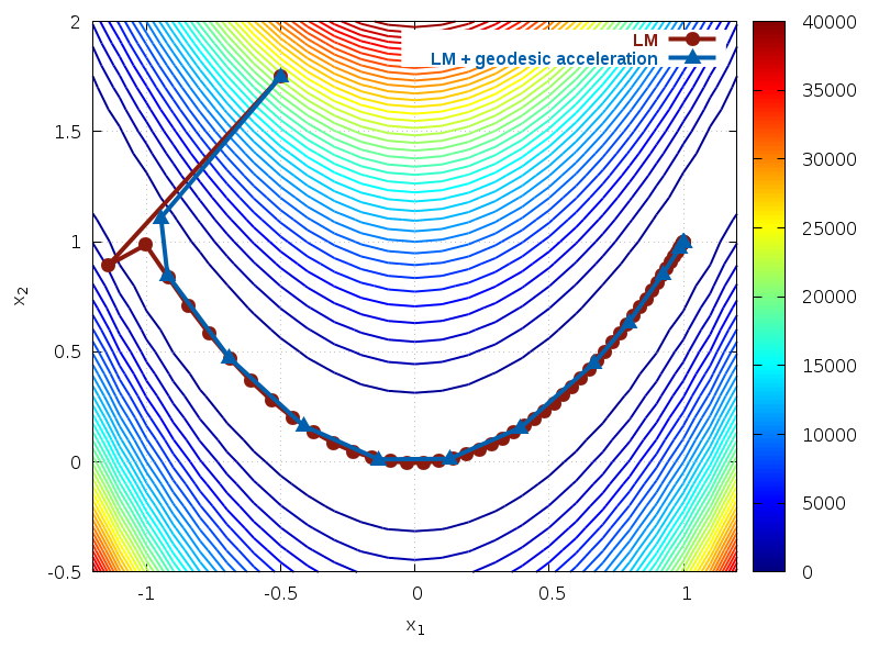
Fig. 37 Paths taken by solver for Rosenbrock function
We can see that enabling geodesic acceleration requires less
than a third of the number of Jacobian evaluations in order to locate
the minimum. The path taken by both methods is shown in Fig. 37.
The contours show the cost function
 . We see that both methods quickly
find the canyon bottom, but the geodesic acceleration method
navigates along the bottom to the solution with significantly
fewer iterations.
. We see that both methods quickly
find the canyon bottom, but the geodesic acceleration method
navigates along the bottom to the solution with significantly
fewer iterations.
The program is given below.
#include <stdlib.h>
#include <stdio.h>
#include <gsl/gsl_vector.h>
#include <gsl/gsl_matrix.h>
#include <gsl/gsl_blas.h>
#include <gsl/gsl_multifit_nlinear.h>
int
func_f (const gsl_vector * x, void *params, gsl_vector * f)
{
double x1 = gsl_vector_get(x, 0);
double x2 = gsl_vector_get(x, 1);
gsl_vector_set(f, 0, 100.0 * (x2 - x1*x1));
gsl_vector_set(f, 1, 1.0 - x1);
return GSL_SUCCESS;
}
int
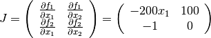
func_df (const gsl_vector * x, void *params, gsl_matrix * J)
{
double x1 = gsl_vector_get(x, 0);
gsl_matrix_set(J, 0, 0, -200.0*x1);
gsl_matrix_set(J, 0, 1, 100.0);
gsl_matrix_set(J, 1, 0, -1.0);
gsl_matrix_set(J, 1, 1, 0.0);
return GSL_SUCCESS;
}
int
func_fvv (const gsl_vector * x, const gsl_vector * v,
void *params, gsl_vector * fvv)
{
double v1 = gsl_vector_get(v, 0);
gsl_vector_set(fvv, 0, -200.0 * v1 * v1);
gsl_vector_set(fvv, 1, 0.0);
return GSL_SUCCESS;
}
void
callback(const size_t iter, void *params,
const gsl_multifit_nlinear_workspace *w)
{
gsl_vector * x = gsl_multifit_nlinear_position(w);
/* print out current location */
printf("%f %f\n",
gsl_vector_get(x, 0),
gsl_vector_get(x, 1));
}
void
solve_system(gsl_vector *x0, gsl_multifit_nlinear_fdf *fdf,
gsl_multifit_nlinear_parameters *params)
{
const gsl_multifit_nlinear_type *T = gsl_multifit_nlinear_trust;
const size_t max_iter = 200;
const double xtol = 1.0e-8;
const double gtol = 1.0e-8;
const double ftol = 1.0e-8;
const size_t n = fdf->n;
const size_t p = fdf->p;
gsl_multifit_nlinear_workspace *work =
gsl_multifit_nlinear_alloc(T, params, n, p);
gsl_vector * f = gsl_multifit_nlinear_residual(work);
gsl_vector * x = gsl_multifit_nlinear_position(work);
int info;
double chisq0, chisq, rcond;
/* initialize solver */
gsl_multifit_nlinear_init(x0, fdf, work);
/* store initial cost */
gsl_blas_ddot(f, f, &chisq0);
/* iterate until convergence */
gsl_multifit_nlinear_driver(max_iter, xtol, gtol, ftol,
callback, NULL, &info, work);
/* store final cost */
gsl_blas_ddot(f, f, &chisq);
/* store cond(J(x)) */
gsl_multifit_nlinear_rcond(&rcond, work);
/* print summary */
fprintf(stderr, "NITER = %zu\n", gsl_multifit_nlinear_niter(work));
fprintf(stderr, "NFEV = %zu\n", fdf->nevalf);
fprintf(stderr, "NJEV = %zu\n", fdf->nevaldf);
fprintf(stderr, "NAEV = %zu\n", fdf->nevalfvv);
fprintf(stderr, "initial cost = %.12e\n", chisq0);
fprintf(stderr, "final cost = %.12e\n", chisq);
fprintf(stderr, "final x = (%.12e, %.12e)\n",
gsl_vector_get(x, 0), gsl_vector_get(x, 1));
fprintf(stderr, "final cond(J) = %.12e\n", 1.0 / rcond);
printf("\n\n");
gsl_multifit_nlinear_free(work);
}
int
main (void)
{
const size_t n = 2;
const size_t p = 2;
gsl_vector *f = gsl_vector_alloc(n);
gsl_vector *x = gsl_vector_alloc(p);
gsl_multifit_nlinear_fdf fdf;
gsl_multifit_nlinear_parameters fdf_params =
gsl_multifit_nlinear_default_parameters();
/* print map of Phi(x1, x2) */
{
double x1, x2, chisq;
double *f1 = gsl_vector_ptr(f, 0);
double *f2 = gsl_vector_ptr(f, 1);
for (x1 = -1.2; x1 < 1.3; x1 += 0.1)
{
for (x2 = -0.5; x2 < 2.1; x2 += 0.1)
{
gsl_vector_set(x, 0, x1);
gsl_vector_set(x, 1, x2);
func_f(x, NULL, f);
chisq = (*f1) * (*f1) + (*f2) * (*f2);
printf("%f %f %f\n", x1, x2, chisq);
}
printf("\n");
}
printf("\n\n");
}
/* define function to be minimized */
fdf.f = func_f;
fdf.df = func_df;
fdf.fvv = func_fvv;
fdf.n = n;
fdf.p = p;
fdf.params = NULL;
/* starting point */
gsl_vector_set(x, 0, -0.5);
gsl_vector_set(x, 1, 1.75);
fprintf(stderr, "=== Solving system without acceleration ===\n");
fdf_params.trs = gsl_multifit_nlinear_trs_lm;
solve_system(x, &fdf, &fdf_params);
fprintf(stderr, "=== Solving system with acceleration ===\n");
fdf_params.trs = gsl_multifit_nlinear_trs_lmaccel;
solve_system(x, &fdf, &fdf_params);
gsl_vector_free(f);
gsl_vector_free(x);
return 0;
}
Geodesic Acceleration Example 2
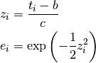
The following example fits a set of data to a Gaussian model using the Levenberg-Marquardt method with geodesic acceleration. The cost function is
where is the measured data point at time  , and
the model is specified by
, and
the model is specified by
![Y(a,b,c;t) = a \exp{
\left[
-{1 \over 2}
\left(
{ t - b \over c }
\right)^2
\right]
}](_images/math/35ca8fbfbbcf8d1ea93a634ae2b37e4db564c0f6.png)
The parameters  represent the amplitude, mean, and width of the Gaussian
respectively. The program below generates the data on
represent the amplitude, mean, and width of the Gaussian
respectively. The program below generates the data on ![[0,1]](_images/math/e7e8ac4ddd4ab0fc62c2a6435f8373f48c776858.png) using
the values
using
the values  ,
,  ,
,  and adding random noise.
The -th row of the Jacobian is
and adding random noise.
The -th row of the Jacobian is

where
In order to use geodesic acceleration, we need the second directional derivative
of the residuals in the velocity direction,
,
where is provided by the solver. To compute this, it is helpful to make a table of
all second derivatives of the residuals with respect to each combination of model parameters.
This table is
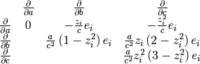
The lower half of the table is omitted since it is symmetric. Then, the second directional derivative
of is

The factors of 2 come from the symmetry of the mixed second partial derivatives.
The iteration is started using the initial guess  .
The program output is shown below:
.
The program output is shown below:
iter  0: a = 1.0000, b = 0.0000, c = 1.0000, |a|/|v| = 0.0000 cond(J) =      inf, |f(x)| = 35.4785
iter  1: a = 1.5708, b = 0.5321, c = 0.5219, |a|/|v| = 0.3093 cond(J) =  29.0443, |f(x)| = 31.1042
iter  2: a = 1.7387, b = 0.4040, c = 0.4568, |a|/|v| = 0.1199 cond(J) =   3.5256, |f(x)| = 28.7217
iter  3: a = 2.2340, b = 0.3829, c = 0.3053, |a|/|v| = 0.3308 cond(J) =   4.5121, |f(x)| = 23.8074
iter  4: a = 3.2275, b = 0.3952, c = 0.2243, |a|/|v| = 0.2784 cond(J) =   8.6499, |f(x)| = 15.6003
iter  5: a = 4.3347, b = 0.3974, c = 0.1752, |a|/|v| = 0.2029 cond(J) =  15.1732, |f(x)| = 7.5908
iter  6: a = 4.9352, b = 0.3992, c = 0.1536, |a|/|v| = 0.1001 cond(J) =  26.6621, |f(x)| = 4.8402
iter  7: a = 5.0716, b = 0.3994, c = 0.1498, |a|/|v| = 0.0166 cond(J) =  34.6922, |f(x)| = 4.7103
iter  8: a = 5.0828, b = 0.3994, c = 0.1495, |a|/|v| = 0.0012 cond(J) =  36.5422, |f(x)| = 4.7095
iter  9: a = 5.0831, b = 0.3994, c = 0.1495, |a|/|v| = 0.0000 cond(J) =  36.6929, |f(x)| = 4.7095
iter 10: a = 5.0831, b = 0.3994, c = 0.1495, |a|/|v| = 0.0000 cond(J) =  36.6975, |f(x)| = 4.7095
iter 11: a = 5.0831, b = 0.3994, c = 0.1495, |a|/|v| = 0.0000 cond(J) =  36.6976, |f(x)| = 4.7095
NITER         = 11
NFEV          = 18
NJEV          = 12
NAEV          = 17
initial cost  = 1.258724737288e+03
final cost    = 2.217977560180e+01
final x       = (5.083101559156e+00, 3.994484109594e-01, 1.494898e-01)
final cond(J) = 3.669757713403e+01
We see the method converges after 11 iterations. For comparison the standard
Levenberg-Marquardt method requires 26 iterations and so the Gaussian fitting
problem benefits substantially from the geodesic acceleration correction. The
column marked |a|/|v| above shows the ratio of the acceleration term
to the velocity term as the iteration progresses. Larger values of this
ratio indicate that the geodesic acceleration correction term is contributing
substantial information to the solver relative to the standard LM velocity step.
The data and fitted model are shown in Fig. 38.
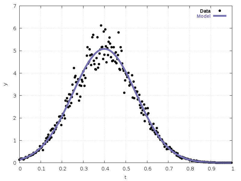
Fig. 38 Gaussian model fitted to data
The program is given below.
#include <stdlib.h>
#include <stdio.h>
#include <gsl/gsl_vector.h>
#include <gsl/gsl_matrix.h>
#include <gsl/gsl_blas.h>
#include <gsl/gsl_multifit_nlinear.h>
#include <gsl/gsl_rng.h>
#include <gsl/gsl_randist.h>

struct data
{
  double *t;
  double *y;
  size_t n;
};

/* model function: a * exp( -1/2 * [ (t - b) / c ]^2 ) */
double
gaussian(const double a, const double b, const double c, const double t)
{
  const double z = (t - b) / c;
  return (a * exp(-0.5 * z * z));
}

int
func_f (const gsl_vector * x, void *params, gsl_vector * f)
{
  struct data *d = (struct data *) params;
  double a = gsl_vector_get(x, 0);
  double b = gsl_vector_get(x, 1);
  double c = gsl_vector_get(x, 2);
  size_t i;

  for (i = 0; i < d->n; ++i)
    {
      double ti = d->t[i];
      double yi = d->y[i];
      double y = gaussian(a, b, c, ti);

      gsl_vector_set(f, i, yi - y);
    }

  return GSL_SUCCESS;
}

int
func_df (const gsl_vector * x, void *params, gsl_matrix * J)
{
  struct data *d = (struct data *) params;
  double a = gsl_vector_get(x, 0);
  double b = gsl_vector_get(x, 1);
  double c = gsl_vector_get(x, 2);
  size_t i;

  for (i = 0; i < d->n; ++i)
    {
      double ti = d->t[i];
      double zi = (ti - b) / c;
      double ei = exp(-0.5 * zi * zi);

      gsl_matrix_set(J, i, 0, -ei);
      gsl_matrix_set(J, i, 1, -(a / c) * ei * zi);
      gsl_matrix_set(J, i, 2, -(a / c) * ei * zi * zi);
    }

  return GSL_SUCCESS;
}

int
func_fvv (const gsl_vector * x, const gsl_vector * v,
          void *params, gsl_vector * fvv)
{
  struct data *d = (struct data *) params;
  double a = gsl_vector_get(x, 0);
  double b = gsl_vector_get(x, 1);
  double c = gsl_vector_get(x, 2);
  double va = gsl_vector_get(v, 0);
  double vb = gsl_vector_get(v, 1);
  double vc = gsl_vector_get(v, 2);
  size_t i;

  for (i = 0; i < d->n; ++i)
    {
      double ti = d->t[i];
      double zi = (ti - b) / c;
      double ei = exp(-0.5 * zi * zi);
      double Dab = -zi * ei / c;
      double Dac = -zi * zi * ei / c;
      double Dbb = a * ei / (c * c) * (1.0 - zi*zi);
      double Dbc = a * zi * ei / (c * c) * (2.0 - zi*zi);
      double Dcc = a * zi * zi * ei / (c * c) * (3.0 - zi*zi);
      double sum;

      sum = 2.0 * va * vb * Dab +
            2.0 * va * vc * Dac +
                  vb * vb * Dbb +
            2.0 * vb * vc * Dbc +
                  vc * vc * Dcc;

      gsl_vector_set(fvv, i, sum);
    }

  return GSL_SUCCESS;
}

void
callback(const size_t iter, void *params,
         const gsl_multifit_nlinear_workspace *w)
{
  gsl_vector *f = gsl_multifit_nlinear_residual(w);
  gsl_vector *x = gsl_multifit_nlinear_position(w);
  double avratio = gsl_multifit_nlinear_avratio(w);
  double rcond;

  (void) params; /* not used */

  /* compute reciprocal condition number of J(x) */
  gsl_multifit_nlinear_rcond(&rcond, w);

  fprintf(stderr, "iter %2zu: a = %.4f, b = %.4f, c = %.4f, |a|/|v| = %.4f cond(J) = %8.4f, |f(x)| = %.4f\n",
          iter,
          gsl_vector_get(x, 0),
          gsl_vector_get(x, 1),
          gsl_vector_get(x, 2),
          avratio,
          1.0 / rcond,
          gsl_blas_dnrm2(f));
}

void
solve_system(gsl_vector *x, gsl_multifit_nlinear_fdf *fdf,
             gsl_multifit_nlinear_parameters *params)
{
  const gsl_multifit_nlinear_type *T = gsl_multifit_nlinear_trust;
  const size_t max_iter = 200;
  const double xtol = 1.0e-8;
  const double gtol = 1.0e-8;
  const double ftol = 1.0e-8;
  const size_t n = fdf->n;
  const size_t p = fdf->p;
  gsl_multifit_nlinear_workspace *work =
    gsl_multifit_nlinear_alloc(T, params, n, p);
  gsl_vector * f = gsl_multifit_nlinear_residual(work);
  gsl_vector * y = gsl_multifit_nlinear_position(work);
  int info;
  double chisq0, chisq, rcond;

  /* initialize solver */
  gsl_multifit_nlinear_init(x, fdf, work);

  /* store initial cost */
  gsl_blas_ddot(f, f, &chisq0);

  /* iterate until convergence */
  gsl_multifit_nlinear_driver(max_iter, xtol, gtol, ftol,
                              callback, NULL, &info, work);

  /* store final cost */
  gsl_blas_ddot(f, f, &chisq);

  /* store cond(J(x)) */
  gsl_multifit_nlinear_rcond(&rcond, work);

  gsl_vector_memcpy(x, y);

  /* print summary */

  fprintf(stderr, "NITER         = %zu\n", gsl_multifit_nlinear_niter(work));
  fprintf(stderr, "NFEV          = %zu\n", fdf->nevalf);
  fprintf(stderr, "NJEV          = %zu\n", fdf->nevaldf);
  fprintf(stderr, "NAEV          = %zu\n", fdf->nevalfvv);
  fprintf(stderr, "initial cost  = %.12e\n", chisq0);
  fprintf(stderr, "final cost    = %.12e\n", chisq);
  fprintf(stderr, "final x       = (%.12e, %.12e, %12e)\n",
          gsl_vector_get(x, 0), gsl_vector_get(x, 1), gsl_vector_get(x, 2));
  fprintf(stderr, "final cond(J) = %.12e\n", 1.0 / rcond);

  gsl_multifit_nlinear_free(work);
}

int
main (void)
{
  const size_t n = 300;  /* number of data points to fit */
  const size_t p = 3;    /* number of model parameters */
  const double a = 5.0;  /* amplitude */
  const double b = 0.4;  /* center */
  const double c = 0.15; /* width */
  const gsl_rng_type * T = gsl_rng_default;
  gsl_vector *f = gsl_vector_alloc(n);
  gsl_vector *x = gsl_vector_alloc(p);
  gsl_multifit_nlinear_fdf fdf;
  gsl_multifit_nlinear_parameters fdf_params =
    gsl_multifit_nlinear_default_parameters();
  struct data fit_data;
  gsl_rng * r;
  size_t i;

  gsl_rng_env_setup ();
  r = gsl_rng_alloc (T);

  fit_data.t = malloc(n * sizeof(double));
  fit_data.y = malloc(n * sizeof(double));
  fit_data.n = n;

  /* generate synthetic data with noise */
  for (i = 0; i < n; ++i)
    {
      double t = (double)i / (double) n;
      double y0 = gaussian(a, b, c, t);
      double dy = gsl_ran_gaussian (r, 0.1 * y0);

      fit_data.t[i] = t;
      fit_data.y[i] = y0 + dy;
    }

  /* define function to be minimized */
  fdf.f = func_f;
  fdf.df = func_df;
  fdf.fvv = func_fvv;
  fdf.n = n;
  fdf.p = p;
  fdf.params = &fit_data;

  /* starting point */
  gsl_vector_set(x, 0, 1.0);
  gsl_vector_set(x, 1, 0.0);
  gsl_vector_set(x, 2, 1.0);

  fdf_params.trs = gsl_multifit_nlinear_trs_lmaccel;
  solve_system(x, &fdf, &fdf_params);

  /* print data and model */
  {
    double A = gsl_vector_get(x, 0);
    double B = gsl_vector_get(x, 1);
    double C = gsl_vector_get(x, 2);

    for (i = 0; i < n; ++i)
      {
        double ti = fit_data.t[i];
        double yi = fit_data.y[i];
        double fi = gaussian(A, B, C, ti);

        printf("%f %f %f\n", ti, yi, fi);
      }
  }

  gsl_vector_free(f);
  gsl_vector_free(x);
  gsl_rng_free(r);

  return 0;
}
Comparing TRS Methods Example
The following program compares all available nonlinear least squares trust-region subproblem (TRS) methods on the Branin function, a common optimization test problem. The cost function is
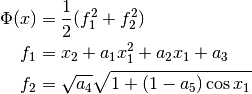
with  .
There are three minima of this function in the range
.
There are three minima of this function in the range
![(x_1,x_2) \in [-5,15] \times [-5,15]](_images/math/78237ab11b0780ef40099205173c822e4d062f08.png) . The program
below uses the starting point
. The program
below uses the starting point  and calculates the solution with all available nonlinear
least squares TRS methods. The program output is shown below:
and calculates the solution with all available nonlinear
least squares TRS methods. The program output is shown below:
Method                    NITER  NFEV  NJEV  Initial Cost  Final cost   Final cond(J) Final x
levenberg-marquardt       20     27    21    1.9874e+02    3.9789e-01   6.1399e+07    (-3.14e+00, 1.23e+01)
levenberg-marquardt+accel 27     36    28    1.9874e+02    3.9789e-01   1.4465e+07    (3.14e+00, 2.27e+00)
dogleg                    23     64    23    1.9874e+02    3.9789e-01   5.0692e+08    (3.14e+00, 2.28e+00)
double-dogleg             24     69    24    1.9874e+02    3.9789e-01   3.4879e+07    (3.14e+00, 2.27e+00)
2D-subspace               23     54    24    1.9874e+02    3.9789e-01   2.5142e+07    (3.14e+00, 2.27e+00)
The first row of output above corresponds to standard Levenberg-Marquardt, while
the second row includes geodesic acceleration. We see that the standard LM method
converges to the minimum at  and also uses the least number
of iterations and Jacobian evaluations. All other methods converge to the minimum
and also uses the least number
of iterations and Jacobian evaluations. All other methods converge to the minimum
 and perform similarly in terms of number of Jacobian evaluations.
We see that is fairly ill-conditioned
at both minima, indicating that the QR (or SVD) solver is the best choice for this problem.
Since there are only two parameters in this optimization problem, we can easily
visualize the paths taken by each method, which are shown in Fig. 39.
The figure shows contours of the cost function which exhibits
three global minima in the range
and perform similarly in terms of number of Jacobian evaluations.
We see that is fairly ill-conditioned
at both minima, indicating that the QR (or SVD) solver is the best choice for this problem.
Since there are only two parameters in this optimization problem, we can easily
visualize the paths taken by each method, which are shown in Fig. 39.
The figure shows contours of the cost function which exhibits
three global minima in the range ![[-5,15] \times [-5,15]](_images/math/71a226b4498f2c8629075cf73bcca67c0f17f435.png) . The paths taken
by each solver are shown as colored lines.
. The paths taken
by each solver are shown as colored lines.
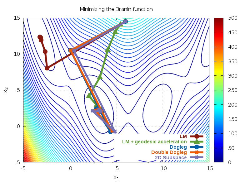
Fig. 39 Paths taken for different TRS methods for the Branin function
The program is given below.
#include <stdlib.h>
#include <stdio.h>
#include <gsl/gsl_vector.h>
#include <gsl/gsl_matrix.h>
#include <gsl/gsl_blas.h>
#include <gsl/gsl_multifit_nlinear.h>
/* parameters to model */
struct model_params
{
double a1;
double a2;
double a3;
double a4;
double a5;
};
/* Branin function */
int
func_f (const gsl_vector * x, void *params, gsl_vector * f)
{
struct model_params *par = (struct model_params *) params;
double x1 = gsl_vector_get(x, 0);
double x2 = gsl_vector_get(x, 1);
double f1 = x2 + par->a1 * x1 * x1 + par->a2 * x1 + par->a3;
double f2 = sqrt(par->a4) * sqrt(1.0 + (1.0 - par->a5) * cos(x1));
gsl_vector_set(f, 0, f1);
gsl_vector_set(f, 1, f2);
return GSL_SUCCESS;
}
int
func_df (const gsl_vector * x, void *params, gsl_matrix * J)
{
struct model_params *par = (struct model_params *) params;
double x1 = gsl_vector_get(x, 0);
double f2 = sqrt(par->a4) * sqrt(1.0 + (1.0 - par->a5) * cos(x1));
gsl_matrix_set(J, 0, 0, 2.0 * par->a1 * x1 + par->a2);
gsl_matrix_set(J, 0, 1, 1.0);
gsl_matrix_set(J, 1, 0, -0.5 * par->a4 / f2 * (1.0 - par->a5) * sin(x1));
gsl_matrix_set(J, 1, 1, 0.0);
return GSL_SUCCESS;
}
int
func_fvv (const gsl_vector * x, const gsl_vector * v,
void *params, gsl_vector * fvv)
{
struct model_params *par = (struct model_params *) params;
double x1 = gsl_vector_get(x, 0);
double v1 = gsl_vector_get(v, 0);
double c = cos(x1);
double s = sin(x1);
double f2 = sqrt(par->a4) * sqrt(1.0 + (1.0 - par->a5) * c);
double t = 0.5 * par->a4 * (1.0 - par->a5) / f2;
gsl_vector_set(fvv, 0, 2.0 * par->a1 * v1 * v1);
gsl_vector_set(fvv, 1, -t * (c + s*s/f2) * v1 * v1);
return GSL_SUCCESS;
}
void
callback(const size_t iter, void *params,
const gsl_multifit_nlinear_workspace *w)
{
gsl_vector * x = gsl_multifit_nlinear_position(w);
double x1 = gsl_vector_get(x, 0);
double x2 = gsl_vector_get(x, 1);
/* print out current location */
printf("%f %f\n", x1, x2);
}
void
solve_system(gsl_vector *x0, gsl_multifit_nlinear_fdf *fdf,
gsl_multifit_nlinear_parameters *params)
{
const gsl_multifit_nlinear_type *T = gsl_multifit_nlinear_trust;
const size_t max_iter = 200;
const double xtol = 1.0e-8;
const double gtol = 1.0e-8;
const double ftol = 1.0e-8;
const size_t n = fdf->n;
const size_t p = fdf->p;
gsl_multifit_nlinear_workspace *work =
gsl_multifit_nlinear_alloc(T, params, n, p);
gsl_vector * f = gsl_multifit_nlinear_residual(work);
gsl_vector * x = gsl_multifit_nlinear_position(work);
int info;
double chisq0, chisq, rcond;
printf("# %s/%s\n",
gsl_multifit_nlinear_name(work),
gsl_multifit_nlinear_trs_name(work));
/* initialize solver */
gsl_multifit_nlinear_init(x0, fdf, work);
/* store initial cost */
gsl_blas_ddot(f, f, &chisq0);
/* iterate until convergence */
gsl_multifit_nlinear_driver(max_iter, xtol, gtol, ftol,
callback, NULL, &info, work);
/* store final cost */
gsl_blas_ddot(f, f, &chisq);
/* store cond(J(x)) */
gsl_multifit_nlinear_rcond(&rcond, work);
/* print summary */
fprintf(stderr, "%-25s %-6zu %-5zu %-5zu %-13.4e %-12.4e %-13.4e (%.2e, %.2e)\n",
gsl_multifit_nlinear_trs_name(work),
gsl_multifit_nlinear_niter(work),
fdf->nevalf,
fdf->nevaldf,
chisq0,
chisq,
1.0 / rcond,
gsl_vector_get(x, 0),
gsl_vector_get(x, 1));
printf("\n\n");
gsl_multifit_nlinear_free(work);
}
int
main (void)
{
const size_t n = 2;
const size_t p = 2;
gsl_vector *f = gsl_vector_alloc(n);
gsl_vector *x = gsl_vector_alloc(p);
gsl_multifit_nlinear_fdf fdf;
gsl_multifit_nlinear_parameters fdf_params =
gsl_multifit_nlinear_default_parameters();
struct model_params params;
params.a1 = -5.1 / (4.0 * M_PI * M_PI);
params.a2 = 5.0 / M_PI;
params.a3 = -6.0;
params.a4 = 10.0;
params.a5 = 1.0 / (8.0 * M_PI);
/* print map of Phi(x1, x2) */
{
double x1, x2, chisq;
for (x1 = -5.0; x1 < 15.0; x1 += 0.1)
{
for (x2 = -5.0; x2 < 15.0; x2 += 0.1)
{
gsl_vector_set(x, 0, x1);
gsl_vector_set(x, 1, x2);
func_f(x, ¶ms, f);
gsl_blas_ddot(f, f, &chisq);
printf("%f %f %f\n", x1, x2, chisq);
}
printf("\n");
}
printf("\n\n");
}
/* define function to be minimized */
fdf.f = func_f;
fdf.df = func_df;
fdf.fvv = func_fvv;
fdf.n = n;
fdf.p = p;
fdf.params = ¶ms;
/* starting point */
gsl_vector_set(x, 0, 6.0);
gsl_vector_set(x, 1, 14.5);
fprintf(stderr, "%-25s %-6s %-5s %-5s %-13s %-12s %-13s %-15s\n",
"Method", "NITER", "NFEV", "NJEV", "Initial Cost",
"Final cost", "Final cond(J)", "Final x");
fdf_params.trs = gsl_multifit_nlinear_trs_lm;
solve_system(x, &fdf, &fdf_params);
fdf_params.trs = gsl_multifit_nlinear_trs_lmaccel;
solve_system(x, &fdf, &fdf_params);
fdf_params.trs = gsl_multifit_nlinear_trs_dogleg;
solve_system(x, &fdf, &fdf_params);
fdf_params.trs = gsl_multifit_nlinear_trs_ddogleg;
solve_system(x, &fdf, &fdf_params);
fdf_params.trs = gsl_multifit_nlinear_trs_subspace2D;
solve_system(x, &fdf, &fdf_params);
gsl_vector_free(f);
gsl_vector_free(x);
return 0;
}
Large Nonlinear Least Squares Example
The following program illustrates the large nonlinear least squares solvers on a system with significant sparse structure in the Jacobian. The cost function is
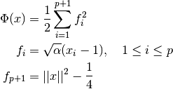
with  . The residual
  imposes a constraint on the
parameters , to ensure that
imposes a constraint on the
parameters , to ensure that  .
The
.
The  -by- Jacobian for this system is
and the normal equations matrix is
Finally, the second directional derivative of for the
geodesic acceleration method is
Since the upper -by- block of is diagonal,
this sparse structure should be exploited in the nonlinear solver.
For comparison, the following program solves the system for  using the dense direct Cholesky solver based on the normal equations matrix
, as well as the iterative Steihaug-Toint solver, based on
sparse matrix-vector products and . The
program output is shown below:
using the dense direct Cholesky solver based on the normal equations matrix
, as well as the iterative Steihaug-Toint solver, based on
sparse matrix-vector products and . The
program output is shown below:
Method                    NITER NFEV NJUEV NJTJEV NAEV Init Cost  Final cost cond(J) Final |x|^2 Time (s)
levenberg-marquardt       25    31   26    26     0    7.1218e+18 1.9555e-02 447.50  2.5044e-01  46.28
levenberg-marquardt+accel 22    23   45    23     22   7.1218e+18 1.9555e-02 447.64  2.5044e-01  33.92
dogleg                    37    87   36    36     0    7.1218e+18 1.9555e-02 447.59  2.5044e-01  56.05
double-dogleg             35    88   34    34     0    7.1218e+18 1.9555e-02 447.62  2.5044e-01  52.65
2D-subspace               37    88   36    36     0    7.1218e+18 1.9555e-02 447.71  2.5044e-01  59.75
steihaug-toint            35    88   345   0      0    7.1218e+18 1.9555e-02 inf     2.5044e-01  0.09
The first five rows use methods based on factoring the dense matrix
while the last row uses the iterative Steihaug-Toint method. While the number
of Jacobian matrix-vector products (NJUEV) is less for the dense methods, the added time
to construct and factor the matrix (NJTJEV) results in a much larger runtime than the
iterative method (see last column).
The program is given below.
#include <stdlib.h>
#include <stdio.h>
#include <sys/time.h>
#include <gsl/gsl_vector.h>
#include <gsl/gsl_matrix.h>
#include <gsl/gsl_blas.h>
#include <gsl/gsl_multilarge_nlinear.h>
#include <gsl/gsl_spblas.h>
#include <gsl/gsl_spmatrix.h>
/* parameters for functions */
struct model_params
{
double alpha;
gsl_spmatrix *J;
};
/* penalty function */
int
penalty_f (const gsl_vector * x, void *params, gsl_vector * f)
{
struct model_params *par = (struct model_params *) params;
const double sqrt_alpha = sqrt(par->alpha);
const size_t p = x->size;
size_t i;
double sum = 0.0;
for (i = 0; i < p; ++i)
{
double xi = gsl_vector_get(x, i);
gsl_vector_set(f, i, sqrt_alpha*(xi - 1.0));
sum += xi * xi;
}
gsl_vector_set(f, p, sum - 0.25);
return GSL_SUCCESS;
}
int
penalty_df (CBLAS_TRANSPOSE_t TransJ, const gsl_vector * x,
const gsl_vector * u, void * params, gsl_vector * v,
gsl_matrix * JTJ)
{
struct model_params *par = (struct model_params *) params;
const size_t p = x->size;
size_t j;
/* store 2*x in last row of J */
for (j = 0; j < p; ++j)
{
double xj = gsl_vector_get(x, j);
gsl_spmatrix_set(par->J, p, j, 2.0 * xj);
}
/* compute v = op(J) u */
if (v)
gsl_spblas_dgemv(TransJ, 1.0, par->J, u, 0.0, v);
if (JTJ)
{
gsl_vector_view diag = gsl_matrix_diagonal(JTJ);
/* compute J^T J = [ alpha*I_p + 4 x x^T ] */
gsl_matrix_set_zero(JTJ);
/* store 4 x x^T in lower half of JTJ */
gsl_blas_dsyr(CblasLower, 4.0, x, JTJ);
/* add alpha to diag(JTJ) */
gsl_vector_add_constant(&diag.vector, par->alpha);
}
return GSL_SUCCESS;
}
int
penalty_fvv (const gsl_vector * x, const gsl_vector * v,
void *params, gsl_vector * fvv)
{
const size_t p = x->size;
double normv = gsl_blas_dnrm2(v);
gsl_vector_set_zero(fvv);
gsl_vector_set(fvv, p, 2.0 * normv * normv);
(void)params; /* avoid unused parameter warning */
return GSL_SUCCESS;
}
void
solve_system(const gsl_vector *x0, gsl_multilarge_nlinear_fdf *fdf,
gsl_multilarge_nlinear_parameters *params)
{
const gsl_multilarge_nlinear_type *T = gsl_multilarge_nlinear_trust;
const size_t max_iter = 200;
const double xtol = 1.0e-8;
const double gtol = 1.0e-8;
const double ftol = 1.0e-8;
const size_t n = fdf->n;
const size_t p = fdf->p;
gsl_multilarge_nlinear_workspace *work =
gsl_multilarge_nlinear_alloc(T, params, n, p);
gsl_vector * f = gsl_multilarge_nlinear_residual(work);
gsl_vector * x = gsl_multilarge_nlinear_position(work);
int info;
double chisq0, chisq, rcond, xsq;
struct timeval tv0, tv1;
gettimeofday(&tv0, NULL);
/* initialize solver */
gsl_multilarge_nlinear_init(x0, fdf, work);
/* store initial cost */
gsl_blas_ddot(f, f, &chisq0);
/* iterate until convergence */
gsl_multilarge_nlinear_driver(max_iter, xtol, gtol, ftol,
NULL, NULL, &info, work);
gettimeofday(&tv1, NULL);
/* store final cost */
gsl_blas_ddot(f, f, &chisq);
/* compute final ||x||^2 */
gsl_blas_ddot(x, x, &xsq);
/* store cond(J(x)) */
gsl_multilarge_nlinear_rcond(&rcond, work);
/* print summary */
fprintf(stderr, "%-25s %-5zu %-4zu %-5zu %-6zu %-4zu %-10.4e %-10.4e %-7.2f %-11.4e %.2f\n",
gsl_multilarge_nlinear_trs_name(work),
gsl_multilarge_nlinear_niter(work),
fdf->nevalf,
fdf->nevaldfu,
fdf->nevaldf2,
fdf->nevalfvv,
chisq0,
chisq,
1.0 / rcond,
xsq,
(tv1.tv_sec - tv0.tv_sec) + 1.0e-6 * (tv1.tv_usec - tv0.tv_usec));
gsl_multilarge_nlinear_free(work);
}
int
main (void)
{
const size_t p = 2000;
const size_t n = p + 1;
gsl_vector *f = gsl_vector_alloc(n);
gsl_vector *x = gsl_vector_alloc(p);
/* allocate sparse Jacobian matrix with 2*p non-zero elements in triplet format */
gsl_spmatrix *J = gsl_spmatrix_alloc_nzmax(n, p, 2 * p, GSL_SPMATRIX_TRIPLET);
gsl_multilarge_nlinear_fdf fdf;
gsl_multilarge_nlinear_parameters fdf_params =
gsl_multilarge_nlinear_default_parameters();
struct model_params params;
size_t i;
params.alpha = 1.0e-5;
params.J = J;
/* define function to be minimized */
fdf.f = penalty_f;
fdf.df = penalty_df;
fdf.fvv = penalty_fvv;
fdf.n = n;
fdf.p = p;
fdf.params = ¶ms;
for (i = 0; i < p; ++i)
{
/* starting point */
gsl_vector_set(x, i, i + 1.0);
/* store sqrt(alpha)*I_p in upper p-by-p block of J */
gsl_spmatrix_set(J, i, i, sqrt(params.alpha));
}
fprintf(stderr, "%-25s %-4s %-4s %-5s %-6s %-4s %-10s %-10s %-7s %-11s %-10s\n",
"Method", "NITER", "NFEV", "NJUEV", "NJTJEV", "NAEV", "Init Cost",
"Final cost", "cond(J)", "Final |x|^2", "Time (s)");
fdf_params.scale = gsl_multilarge_nlinear_scale_levenberg;
fdf_params.trs = gsl_multilarge_nlinear_trs_lm;
solve_system(x, &fdf, &fdf_params);
fdf_params.trs = gsl_multilarge_nlinear_trs_lmaccel;
solve_system(x, &fdf, &fdf_params);
fdf_params.trs = gsl_multilarge_nlinear_trs_dogleg;
solve_system(x, &fdf, &fdf_params);
fdf_params.trs = gsl_multilarge_nlinear_trs_ddogleg;
solve_system(x, &fdf, &fdf_params);
fdf_params.trs = gsl_multilarge_nlinear_trs_subspace2D;
solve_system(x, &fdf, &fdf_params);
fdf_params.trs = gsl_multilarge_nlinear_trs_cgst;
solve_system(x, &fdf, &fdf_params);
gsl_vector_free(f);
gsl_vector_free(x);
gsl_spmatrix_free(J);
return 0;
}
References and Further Reading
The following publications are relevant to the algorithms described in this section,
J.J. Moré, The Levenberg-Marquardt Algorithm: Implementation and Theory, Lecture Notes in Mathematics, v630 (1978), ed G. Watson.
H. B. Nielsen, “Damping Parameter in Marquardt’s Method”, IMM Department of Mathematical Modeling, DTU, Tech. Report IMM-REP-1999-05 (1999).
K. Madsen and H. B. Nielsen, “Introduction to Optimization and Data Fitting”, IMM Department of Mathematical Modeling, DTU, 2010.
J. E. Dennis and R. B. Schnabel, Numerical Methods for Unconstrained Optimization and Nonlinear Equations, SIAM, 1996.
M. K. Transtrum, B. B. Machta, and J. P. Sethna, Geometry of nonlinear least squares with applications to sloppy models and optimization, Phys. Rev. E 83, 036701, 2011.
M. K. Transtrum and J. P. Sethna, Improvements to the Levenberg-Marquardt algorithm for nonlinear least-squares minimization, arXiv:1201.5885, 2012.
J.J. Moré, B.S. Garbow, K.E. Hillstrom, “Testing Unconstrained Optimization Software”, ACM Transactions on Mathematical Software, Vol 7, No 1 (1981), p 17–41.
H. B. Nielsen, “UCTP Test Problems for Unconstrained Optimization”, IMM Department of Mathematical Modeling, DTU, Tech. Report IMM-REP-2000-17 (2000).