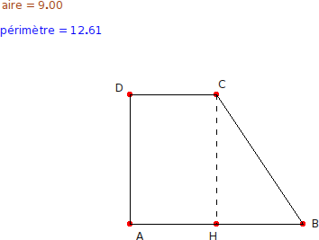
Figure 6.1: Right trapezoid
Next: Various tips, Previous: Smalltalk sketch, Up: Top [Contents][Index]
This chapter is an aid to studying Dr.Geo using didactic examples. Although in the previous chapters several examples were presented, here the approach is little more concrete, while still very original. This chapter was created using contributions from various cultural sources.
One possible didactic use of Dr.Geo is through its Smalltalk script system to resolve classic geometry exercises.
As an example, we will show the solution of the following classic problem – involving the Pythagorean theorem:
A right trapezoid ABCD where the bases and height are known. Calculate its perimeter and area.
Solution:
First we construct the Dr.Geo sketch as follows:
The sketch contains the data to use to resolve the problem. First we can answer the question of the area. To do so we write a Smalltalk script with arguments the two bases and the height:
areaTrapezoidBase1: b1 base2: b2 height: h
"Calculate the area of a right trapezoid given
its bases and one height"
   ^ h length * (b1 length + b2 length) / 2
To calculate the perimeter, we write a script where we calculate the length of BC with the Pythagorean theorem:
perimeterTrapezoidBase1: b1 base2: b2 height: h
"Calculate the area of a right trapezoid given
its two bases and one height"
| hb bc |
   hb := (b2 length - b1 length) abs.
   bc := (hb squared + h length squared) sqrt.
   ^ b1 length + b2 length + h length + bc
It is not difficult, if you follow the same model, to develop other similar examples.
With Smalltalk scripts one can solve exercises, but can also understand theorems more deeply and verify conjectures. In this section we start to analyse Ptolemy’s theorem:
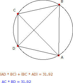
Given an inscribed quadrilateral, the sum of the products of its opposite sides is equal to the product of its diagonals.
We construct the sketch as below where we implemented two scripts to calculate respectively the sum of the products of its opposite sides and the product of its diagonals.
The first script:
ptolemySumS1: ab s2: bc s3: cd s4: ad
"Select the four consecutive sides of the quadrilateral,
then the location for the result"
^ (ad length * bc length) + (ab length * cd length)
The second script:
ptolemyProductD1: ac d2: bd
"Select the two diagonals of the quadrilateral,
then the location for the result"
^ ac length * bd length
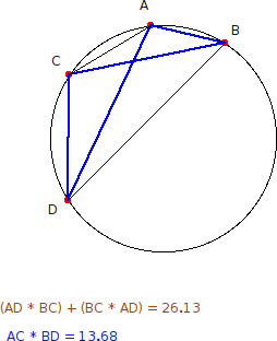
As we can see, the values returned by the scripts, as stated by Ptolemy’s theorem, are equal15 When we dynamically modify the sketch, the script values are always equal, except in the following situation where the quadrilateral is not convex:
In this case the theorem is not true and the previous text of the theorem is inaccurate. It should be reformulated as follow:
Given an inscribed CONVEX quadrilateral, the sum of the products of its opposite sides is equal to the product of its diagonals.
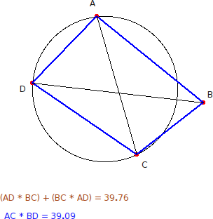
Now a additional conjecture can be stated: is the theorem still valid when the convex quadrilateral is non inscribed?
With Dr.Geo we verify this conjecture is false with the following counterexample bellow. To build this counterexample, we have just detached the point B from the circle by dragging it with the touch Shift pressed at the same time.
The reader will easily use Dr.Geo to construct additional didactic examples, perhaps more famous, relative to the Pythagorean and Euclidean theorems.
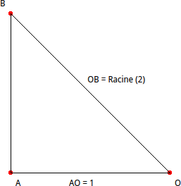
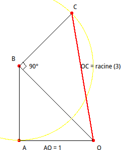
A classic construction of irrational numbers, known as the Teodoro spiral, gives the geometric construction of integer square roots. It begins with an isosceles right triangle.
Let’s start with the triangle OAB where OA=AB=1:
Using the Pythagorean theorem we have OB equal to the square root of 2. Now, with the sketch, we construct another right triangle with the sides OB and BC so that BC=1.
Still using the Pythagorean theorem, it is clear the hypotenuse OC of OBC has a length equal to the square root of 3. The process can be repeated without limit to get the square roots of all positive integers.
The iterative nature of this construction can be naturally represented in a Smalltalk sketch.
Let’s consider the following Smalltalk sketch source code:
| sketch triangle |
sketch := DrGeoCanvas new fullscreen.
triangle := [:p1 :p2 :p3  :n |
   |s1 s2 s3 perp circle p4 |
   s1 := sketch segment: p1 to: p2.
   s2 := (sketch segment: p2 to: p3) color: Color red.
   s3 := sketch segment: p3 to: p1.
   perp := (sketch perpendicular: s3 at: p3) hide.
   circle := (sketch circleCenter: p3 to: p2) hide.
   p4 := (sketch altIntersectionOf: circle and:  perp) hide.
   n > 0 ifTrue: [triangle value: p1 value: p3 value: p4 value: n -1]].

triangle
   value: 0@0
   value: -1@0
   value: -1@1
   value: 50
The triangle at the beginning is defined by the coordinates of its
vertices. The source code is a direct transcription of the logic of
the construction, integrating its iterative nature with a recursive
loop. We use the #hide message several times to mask
intermediate constructions, in order not to overload the user’s
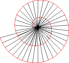
perception with background constructions. Once executed, Dr.Geo
gives the following sketch.
The hypotenuse length of each triangle is the square root of an integer in the interval [2 ; 52].
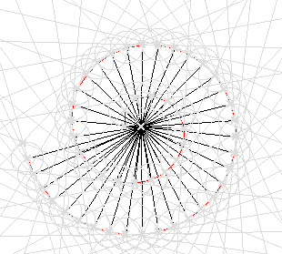
The same spiral with intermediate items shown exposes how difficult it will be to hand construct such a sketch:
As a bonus, here is an animated version of the previous Smalltalk
sketch. To do this we send to the canvas the messages #do: and
#update (See SmalltalkSketchMethods for more reading about
it).
Note the use of the class
Delay to slow down the construction:
| sketch triangle delay|
sketch := DrGeoCanvas new fullscreen.
triangle := [:p1 :p2 :p3  :n |
   |s1 s2 s3 perp circle p4 |
   s1 := sketch segment: p1 to: p2.
   s2 := (sketch segment: p2 to: p3) color: Color red.
   s3 := sketch segment: p3 to: p1.
   perp := sketch perpendicular: s3 at: p3.
   circle := sketch circleCenter: p3 to: p2.
   p4 := sketch altIntersectionOf: circle and:  perp.
   sketch update.
   (Delay forMilliseconds: 200) wait.
   perp hide. circle hide. p4 hide.
   n > 0 ifTrue: [triangle value: p1 value: p3 value: p4 value: n -1]].

sketch do: [triangle value: 0@0 value: -1@0 value: -1@1 value: 50]
As we saw previously, in Smalltalk sketches it is easy to construct, intuitively and simply, sketches to visualise recursive or iterative situations in programming.
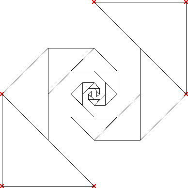
We can go one step further by modifying the previous Smalltalk code – used to construct irrational numbers – to get a famous sketch of the mathematics literature: the Baravelle spiral constructed from similar equilateral right triangles.
The code to construct this spiral is as follows:
| sketch triangle |
sketch := DrGeoCanvas new fullscreen.
triangle := [:p1 :p2 :p3 :n |
   |s1 s2 s3 m  perp circle p4 |
   s1 := sketch segment: p1 to: p2.
   s2 := sketch segment: p2 to: p3.
   s3 := sketch segment: p3 to: p1.
   m := (sketch middleOf: p1 and: p3) hide.
   perp := (sketch perpendicular: s3 at: p3) hide.
   circle := (sketch
      circleCenter: p3
      radius: (sketch distance: m to: p3) hide) hide.
   p4 := (sketch altIntersectionOf: circle and: perp) hide.
   n > 0 ifTrue: [triangle value: m value: p3 value: p4 value: n -1]
].

triangle
   value: (sketch point: 0@5)
   value: (sketch point: 5@5)
   value: (sketch point: 5@0)
   value: 9.
triangle
   value: (sketch point: 0@ -5)
   value: (sketch point: -5@ -5)
   value: (sketch point: -5@0)
   value: 9
With this sketch and the corresponding Smalltalk code we clearly perceive the recursive nature of the construction mechanism. An interesting problem for the reader is to establish when the two branches of the spiral converge.
Another classic use of a Smalltalk programmed sketch is based on its numeric ability to reproduce a geometric sketch knowing its analytic characteristics.
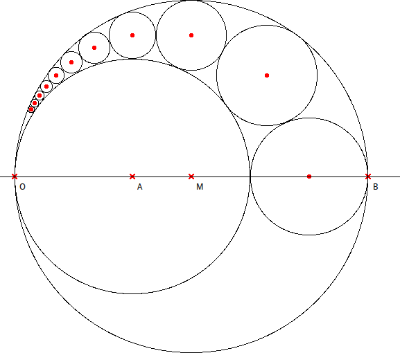
The example we propose is the famous “Pappus Chain”.
The successive circles’ centres and radii are analytically known, and in fact rational. It is therefore easy to reproduce this sketch by programming.
| sketch circle a o m|
sketch := DrGeoCanvas new fullscreen.
circle := [:n |
   | r c p |
   r := (sketch freeValue: 15 / (n squared + 6)) hide.
   c := sketch point:
     (15 / (n squared + 6) * 5) @
     (15 / (n squared + 6) * n * 2).
   c small; round.
   p := sketch circleCenter: c radius: r.
   n > 0 ifTrue: [circle value: n - 1]].

circle value: 10 .
a := (sketch point: 5@0) name: 'A'.
o := (sketch point: 0@0) name: 'O'.
m := sketch
   middleOf: o
   and: ((sketch point: 15@0) name: 'B').
m name: 'M'.
sketch
   circleCenter: m to: o;
   circleCenter: a to: o;
   line: a to: o.
The source code is relatively intuitive and it does not require any comment.
A non-trivial exercise for the reader consists of determining a ruler and compass construction for the figure.
The approximation of pi played an important role in the history of mathematics. Numerous methods were proposed, offering a variety of improvements over time, from elementary geometry to calculus. We will examine one of the earliest approaches to the problem, originally carried out by Archimedes, called – although this phrase is not precisely accurate – the method of exhaustion. This approach has however the advantage of exposing the essence of the methodology.
Archimedes described a simple ruler and compass construction of regular polygons inscribed inside and outside a circle, and laborious calculations of the lengths of their sides, doubling the number of sides at each step up to 96. In modern terms, this gives three digits of precision, approximately 3.14. We, however, can proceed much more simply, letting Dr.Geo do the hard work, and continuing to polygons of more than a million sides, which takes us nearly to the limits of ordinary computer arithmetic, that is, 16 decimal places for floating point numbers (3.141592653589793). Using much more advanced methods on supercomputers has made it possible to calculate ten trillion digits of pi.
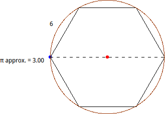
We start with the construction of an inscribed regular hexagon. Create a numeric value, and set it to 6. Create a segment (the diameter) and bisect it to get the center. Create a circle with the given center through one of the endpoints of the segment. Create a regular polygon with the given center, one of the endpoints as a vertex, and the numeric value as the number of sides.
The idea of the of the exhaustion method starts with approximating the length of the circle with the perimeter of the P0 hexagon; then to calculate an approximation of pi as the quotient of the perimeter of that hexagon by the diameter of the circle. Clearly, since the side of the hexagon is the same length as the radius of the circle, the resulting initial approximation of pi is 3.
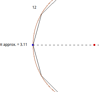
In a second step, we construct an inscribed dodecagon. To construct the previous regular hexagon, we used the Dr.Geo tool to construct a regular polygon with 6 vertices. To construct the dodecagon, we just need to change this free value item to 12, and the polygon will update automatically. We calculate the P1 perimeter, then an approximation of pi as the quotient of the perimeter by the diameter of the circle.
A small script is written to calculate this quotient; its arguments are the polygon and the circle diameter:
approxPIpolygon: poly diameter: d
"PI approximation given an inscribed regular polygon.
Arguments: the polygon and the circle diameter"
   ^ poly length / d length
Now apply this script to the constructed polygon and its diameter (the segment we started with), and pin the result in the sketch.
When increasing the number of sides of the polygon, by editing the free value, we improve the approximation.
To display both the approximation of pi and its accuracy, we can modify the script to display them together:
approxPIpolygon: poly diameter: d
"PI approximation given an inscribed regular polygon.
Arguments: the polygon and the circle diameter"
^ Array
   with: poly length / d length
   with: (poly length / d length - Float pi) abs
As we increase the number of sides of the polygon, how quickly does this process approach the true value? How far can we go?
Next: Various tips, Previous: Smalltalk sketch, Up: Top [Contents][Index]