Discrete Hankel Transforms
This chapter describes functions for performing Discrete Hankel
Transforms (DHTs). The functions are declared in the header file
gsl_dht.h.
Definitions
The discrete Hankel transform acts on a vector of sampled data, where the samples are assumed to have been taken at points related to the zeros of a Bessel function of fixed order; compare this to the case of the discrete Fourier transform, where samples are taken at points related to the zeroes of the sine or cosine function.
Starting with its definition, the Hankel transform (or Bessel transform) of
order  of a function
  with
with  is defined as
(see Johnson, 1987 and Lemoine, 1994)
is defined as
(see Johnson, 1987 and Lemoine, 1994)
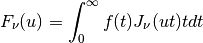
If the integral exists,  is called the Hankel transformation
of . The reverse transform is given by
is called the Hankel transformation
of . The reverse transform is given by
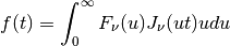
where  must exist and be
absolutely convergent, and where
must exist and be
absolutely convergent, and where  satisfies Dirichlet’s
conditions (of limited total fluctuations) in the interval
satisfies Dirichlet’s
conditions (of limited total fluctuations) in the interval
![[0,\infty]](_images/math/1571bc4591ab1dadc54897ac1b6d5a156bfbe988.png) .
.
Now the discrete Hankel transform works on a discrete function
, which is sampled on points  located at
positions
located at
positions 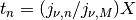 in real space and
at
in real space and
at  in reciprocal space. Here,
 are the m-th zeros of the Bessel function
 arranged in ascending order. Moreover, the
discrete functions are assumed to be band limited, so
arranged in ascending order. Moreover, the
discrete functions are assumed to be band limited, so
 and
and  for
for  . Accordingly,
the function is defined on the interval
. Accordingly,
the function is defined on the interval ![[0,X]](_images/math/0b5c231d65bdf35281a05c6e1ed4c13d87114aad.png) .
.
Following the work of Johnson, 1987 and Lemoine, 1994, the discrete Hankel transform is given by
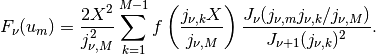
It is this discrete expression which defines the discrete Hankel
transform calculated by GSL. In GSL, forward and backward transforms
are defined equally and calculate  .
Following Johnson, the backward transform reads
.
Following Johnson, the backward transform reads
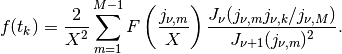
Obviously, using the forward transform instead of the backward transform gives an
additional factor 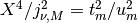 .
.
The kernel in the summation above defines the matrix of the
-Hankel transform of size  . The coefficients of
this matrix, being dependent on and
. The coefficients of
this matrix, being dependent on and  , must be
precomputed and stored; the
, must be
precomputed and stored; the gsl_dht object encapsulates this
data. The allocation function gsl_dht_alloc() returns a
gsl_dht object which must be properly initialized with
gsl_dht_init() before it can be used to perform transforms on data
sample vectors, for fixed and , using the
gsl_dht_apply() function. The implementation allows to define the
length  of the fundamental interval, for convenience, while
discrete Hankel transforms are often defined on the unit interval
instead of .
of the fundamental interval, for convenience, while
discrete Hankel transforms are often defined on the unit interval
instead of .
Notice that by assumption vanishes at the endpoints
of the interval, consistent with the inversion formula
and the sampling formula given above. Therefore, this transform
corresponds to an orthogonal expansion in eigenfunctions
of the Dirichlet problem for the Bessel differential equation.
Functions
-
type gsl_dht
Workspace for computing discrete Hankel transforms
-
gsl_dht *gsl_dht_alloc(size_t size)
This function allocates a Discrete Hankel transform object of size
size.
-
int gsl_dht_init(gsl_dht *t, double nu, double xmax)
This function initializes the transform
tfor the given values ofnuandxmax.
-
gsl_dht *gsl_dht_new(size_t size, double nu, double xmax)
This function allocates a Discrete Hankel transform object of size
sizeand initializes it for the given values ofnuandxmax.
-
int gsl_dht_apply(const gsl_dht *t, double *f_in, double *f_out)
This function applies the transform
tto the arrayf_inwhose size is equal to the size of the transform. The result is stored in the arrayf_outwhich must be of the same length.Applying this function to its output gives the original data multiplied by
 ,
up to numerical errors.
,
up to numerical errors.
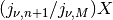 .
These are the points where the function
.
These are the points where the function  .
.References and Further Reading
The algorithms used by these functions are described in the following papers,
Fisk Johnson, Comp.: Phys.: Comm.: 43, 181 (1987).
Lemoine, J. Chem.: Phys.: 101, 3936 (1994).