One Dimensional Root-Finding
This chapter describes routines for finding roots of arbitrary one-dimensional functions. The library provides low level components for a variety of iterative solvers and convergence tests. These can be combined by the user to achieve the desired solution, with full access to the intermediate steps of the iteration. Each class of methods uses the same framework, so that you can switch between solvers at runtime without needing to recompile your program. Each instance of a solver keeps track of its own state, allowing the solvers to be used in multi-threaded programs.
The header file gsl_roots.h contains prototypes for the root
finding functions and related declarations.
Overview
One-dimensional root finding algorithms can be divided into two classes, root bracketing and root polishing. Algorithms which proceed by bracketing a root are guaranteed to converge. Bracketing algorithms begin with a bounded region known to contain a root. The size of this bounded region is reduced, iteratively, until it encloses the root to a desired tolerance. This provides a rigorous error estimate for the location of the root.
The technique of root polishing attempts to improve an initial guess to the root. These algorithms converge only if started “close enough” to a root, and sacrifice a rigorous error bound for speed. By approximating the behavior of a function in the vicinity of a root they attempt to find a higher order improvement of an initial guess. When the behavior of the function is compatible with the algorithm and a good initial guess is available a polishing algorithm can provide rapid convergence.
In GSL both types of algorithm are available in similar frameworks. The user provides a high-level driver for the algorithms, and the library provides the individual functions necessary for each of the steps. There are three main phases of the iteration. The steps are,
initialize solver state,
s, for algorithmTupdate
susing the iterationTtest
sfor convergence, and repeat iteration if necessary
The state for bracketing solvers is held in a gsl_root_fsolver
struct. The updating procedure uses only function evaluations (not
derivatives). The state for root polishing solvers is held in a
gsl_root_fdfsolver struct. The updates require both the function
and its derivative (hence the name fdf) to be supplied by the
user.
Caveats
Note that root finding functions can only search for one root at a time. When there are several roots in the search area, the first root to be found will be returned; however it is difficult to predict which of the roots this will be. In most cases, no error will be reported if you try to find a root in an area where there is more than one.
Care must be taken when a function may have a multiple root (such as
 or
or
 .
It is not possible to use root-bracketing algorithms on
even-multiplicity roots. For these algorithms the initial interval must
contain a zero-crossing, where the function is negative at one end of
the interval and positive at the other end. Roots with even-multiplicity
do not cross zero, but only touch it instantaneously. Algorithms based
on root bracketing will still work for odd-multiplicity roots
(e.g. cubic, quintic, …).
Root polishing algorithms generally work with higher multiplicity roots,
but at a reduced rate of convergence. In these cases the Steffenson
algorithm can be used to accelerate the convergence of multiple roots.
.
It is not possible to use root-bracketing algorithms on
even-multiplicity roots. For these algorithms the initial interval must
contain a zero-crossing, where the function is negative at one end of
the interval and positive at the other end. Roots with even-multiplicity
do not cross zero, but only touch it instantaneously. Algorithms based
on root bracketing will still work for odd-multiplicity roots
(e.g. cubic, quintic, …).
Root polishing algorithms generally work with higher multiplicity roots,
but at a reduced rate of convergence. In these cases the Steffenson
algorithm can be used to accelerate the convergence of multiple roots.
While it is not absolutely required that  have a root within the
search region, numerical root finding functions should not be used
haphazardly to check for the existence of roots. There are better
ways to do this. Because it is easy to create situations where numerical
root finders can fail, it is a bad idea to throw a root finder at a
function you do not know much about. In general it is best to examine
the function visually by plotting before searching for a root.
have a root within the
search region, numerical root finding functions should not be used
haphazardly to check for the existence of roots. There are better
ways to do this. Because it is easy to create situations where numerical
root finders can fail, it is a bad idea to throw a root finder at a
function you do not know much about. In general it is best to examine
the function visually by plotting before searching for a root.
Initializing the Solver
-
type gsl_root_fsolver
This is a workspace for finding roots using methods which do not require derivatives.
-
type gsl_root_fdfsolver
This is a workspace for finding roots using methods which require derivatives.
-
gsl_root_fsolver *gsl_root_fsolver_alloc(const gsl_root_fsolver_type *T)
This function returns a pointer to a newly allocated instance of a solver of type
T. For example, the following code creates an instance of a bisection solver:const gsl_root_fsolver_type * T = gsl_root_fsolver_bisection; gsl_root_fsolver * s = gsl_root_fsolver_alloc (T);
If there is insufficient memory to create the solver then the function returns a null pointer and the error handler is invoked with an error code of
GSL_ENOMEM.
-
gsl_root_fdfsolver *gsl_root_fdfsolver_alloc(const gsl_root_fdfsolver_type *T)
This function returns a pointer to a newly allocated instance of a derivative-based solver of type
T. For example, the following code creates an instance of a Newton-Raphson solver:const gsl_root_fdfsolver_type * T = gsl_root_fdfsolver_newton; gsl_root_fdfsolver * s = gsl_root_fdfsolver_alloc (T);
If there is insufficient memory to create the solver then the function returns a null pointer and the error handler is invoked with an error code of
GSL_ENOMEM.
-
int gsl_root_fsolver_set(gsl_root_fsolver *s, gsl_function *f, double x_lower, double x_upper)
This function initializes, or reinitializes, an existing solver
sto use the functionfand the initial search interval [x_lower,x_upper].
-
int gsl_root_fdfsolver_set(gsl_root_fdfsolver *s, gsl_function_fdf *fdf, double root)
This function initializes, or reinitializes, an existing solver
sto use the function and derivativefdfand the initial guessroot.
-
void gsl_root_fsolver_free(gsl_root_fsolver *s)
-
void gsl_root_fdfsolver_free(gsl_root_fdfsolver *s)
These functions free all the memory associated with the solver
s.
-
const char *gsl_root_fsolver_name(const gsl_root_fsolver *s)
-
const char *gsl_root_fdfsolver_name(const gsl_root_fdfsolver *s)
These functions return a pointer to the name of the solver. For example:
printf ("s is a '%s' solver\n", gsl_root_fsolver_name (s));
would print something like
s is a 'bisection' solver.
Providing the function to solve
You must provide a continuous function of one variable for the root finders to operate on, and, sometimes, its first derivative. In order to allow for general parameters the functions are defined by the following data types:
-
type gsl_function
This data type defines a general function with parameters.
double (* function) (double x, void * params)this function should return the value
 for argument
 xand parametersparamsvoid * paramsa pointer to the parameters of the function
Here is an example for the general quadratic function,
with  ,
,  ,
,  . The following code
defines a
. The following code
defines a gsl_function F which you could pass to a root
finder as a function pointer:
struct my_f_params { double a; double b; double c; };
double
my_f (double x, void * p)
{
struct my_f_params * params = (struct my_f_params *)p;
double a = (params->a);
double b = (params->b);
double c = (params->c);
return (a * x + b) * x + c;
}
gsl_function F;
struct my_f_params params = { 3.0, 2.0, 1.0 };
F.function = &my_f;
F.params = ¶ms;
The function  can be evaluated using the macro
GSL_FN_EVAL(&F,x) defined in gsl_math.h.
-
type gsl_function_fdf
This data type defines a general function with parameters and its first derivative.
double (* f) (double x, void * params)this function should return the value of
for argument xand parametersparamsdouble (* df) (double x, void * params)this function should return the value of the derivative of
fwith respect tox, , for argument
 xand parametersparamsvoid (* fdf) (double x, void * params, double * f, double * df)this function should set the values of the function
fto
and its derivative dfto
for argument xand parametersparams. This function provides an optimization of the separate functions for and
 —it is always faster to compute the function and its
derivative at the same time.
—it is always faster to compute the function and its
derivative at the same time.void * paramsa pointer to the parameters of the function
Here is an example where
 :
:
double
my_f (double x, void * params)
{
   return exp (2 * x);
}

double
my_df (double x, void * params)
{
   return 2 * exp (2 * x);
}

void
my_fdf (double x, void * params,
        double * f, double * df)
{
   double t = exp (2 * x);

   *f = t;
   *df = 2 * t;   /* uses existing value */
}

gsl_function_fdf FDF;

FDF.f = &my_f;
FDF.df = &my_df;
FDF.fdf = &my_fdf;
FDF.params = 0;
The function can be evaluated using the macro
GSL_FN_FDF_EVAL_F(&FDF,x) and the derivative can
be evaluated using the macro GSL_FN_FDF_EVAL_DF(&FDF,x). Both
the function  and its derivative
  can
be evaluated at the same time using the macro
can
be evaluated at the same time using the macro
GSL_FN_FDF_EVAL_F_DF(&FDF,x,y,dy). The macro stores
in its y argument and in its dy
argument—both of these should be pointers to double.
Search Bounds and Guesses
You provide either search bounds or an initial guess; this section explains how search bounds and guesses work and how function arguments control them.
A guess is simply an  value which is iterated until it is within
the desired precision of a root. It takes the form of a
value which is iterated until it is within
the desired precision of a root. It takes the form of a double.
Search bounds are the endpoints of an interval which is iterated until the length of the interval is smaller than the requested precision. The interval is defined by two values, the lower limit and the upper limit. Whether the endpoints are intended to be included in the interval or not depends on the context in which the interval is used.
Iteration
The following functions drive the iteration of each algorithm. Each function performs one iteration to update the state of any solver of the corresponding type. The same functions work for all solvers so that different methods can be substituted at runtime without modifications to the code.
-
int gsl_root_fsolver_iterate(gsl_root_fsolver *s)
-
int gsl_root_fdfsolver_iterate(gsl_root_fdfsolver *s)
These functions perform a single iteration of the solver
s. If the iteration encounters an unexpected problem then an error code will be returned,GSL_EBADFUNCthe iteration encountered a singular point where the function or its derivative evaluated to
InforNaN.GSL_EZERODIVthe derivative of the function vanished at the iteration point, preventing the algorithm from continuing without a division by zero.
The solver maintains a current best estimate of the root at all times. The bracketing solvers also keep track of the current best interval bounding the root. This information can be accessed with the following auxiliary functions,
-
double gsl_root_fsolver_root(const gsl_root_fsolver *s)
-
double gsl_root_fdfsolver_root(const gsl_root_fdfsolver *s)
These functions return the current estimate of the root for the solver
s.
-
double gsl_root_fsolver_x_lower(const gsl_root_fsolver *s)
-
double gsl_root_fsolver_x_upper(const gsl_root_fsolver *s)
These functions return the current bracketing interval for the solver
s.
Search Stopping Parameters
A root finding procedure should stop when one of the following conditions is true:
A root has been found to within the user-specified precision.
A user-specified maximum number of iterations has been reached.
An error has occurred.
The handling of these conditions is under user control. The functions below allow the user to test the precision of the current result in several standard ways.
-
int gsl_root_test_interval(double x_lower, double x_upper, double epsabs, double epsrel)
This function tests for the convergence of the interval [
x_lower,x_upper] with absolute errorepsabsand relative errorepsrel. The test returnsGSL_SUCCESSif the following condition is achieved,
when the interval
![x = [a,b]](_images/math/b7dfd6c9d58c7a97d19cba79a64601e86331937f.png) does not include the origin. If the
interval includes the origin then
does not include the origin. If the
interval includes the origin then  is replaced by
zero (which is the minimum value of
is replaced by
zero (which is the minimum value of  over the interval). This
ensures that the relative error is accurately estimated for roots close
to the origin.
over the interval). This
ensures that the relative error is accurately estimated for roots close
to the origin.This condition on the interval also implies that any estimate of the root
 in the interval satisfies the same condition with respect
to the true root
in the interval satisfies the same condition with respect
to the true root  ,
,
assuming that the true root
is contained within the interval.
-
int gsl_root_test_delta(double x1, double x0, double epsabs, double epsrel)
This function tests for the convergence of the sequence
x0,x1with absolute errorepsabsand relative errorepsrel. The test returnsGSL_SUCCESSif the following condition is achieved,
and returns
GSL_CONTINUEotherwise.
-
int gsl_root_test_residual(double f, double epsabs)
This function tests the residual value
fagainst the absolute error boundepsabs. The test returnsGSL_SUCCESSif the following condition is achieved,
and returns
GSL_CONTINUEotherwise. This criterion is suitable for situations where the precise location of the root,, is
unimportant provided a value can be found where the residual,
 , is small enough.
Root Bracketing Algorithms
The root bracketing algorithms described in this section require an
initial interval which is guaranteed to contain a root—if  and
and  are the endpoints of the interval then
  must
differ in sign from
must
differ in sign from  . This ensures that the function crosses
zero at least once in the interval. If a valid initial interval is used
then these algorithm cannot fail, provided the function is well-behaved.
. This ensures that the function crosses
zero at least once in the interval. If a valid initial interval is used
then these algorithm cannot fail, provided the function is well-behaved.
Note that a bracketing algorithm cannot find roots of even degree, since
these do not cross the -axis.
-
type gsl_root_fsolver_type
-
gsl_root_fsolver_type *gsl_root_fsolver_bisection
The bisection algorithm is the simplest method of bracketing the roots of a function. It is the slowest algorithm provided by the library, with linear convergence.
On each iteration, the interval is bisected and the value of the function at the midpoint is calculated. The sign of this value is used to determine which half of the interval does not contain a root. That half is discarded to give a new, smaller interval containing the root. This procedure can be continued indefinitely until the interval is sufficiently small.
At any time the current estimate of the root is taken as the midpoint of the interval.
-
gsl_root_fsolver_type *gsl_root_fsolver_falsepos
The false position algorithm is a method of finding roots based on linear interpolation. Its convergence is linear, but it is usually faster than bisection.
On each iteration a line is drawn between the endpoints
 and
and  and the point where this line crosses the
-axis taken as a “midpoint”. The value of the function at
this point is calculated and its sign is used to determine which side of
the interval does not contain a root. That side is discarded to give a
new, smaller interval containing the root. This procedure can be
continued indefinitely until the interval is sufficiently small.
and the point where this line crosses the
-axis taken as a “midpoint”. The value of the function at
this point is calculated and its sign is used to determine which side of
the interval does not contain a root. That side is discarded to give a
new, smaller interval containing the root. This procedure can be
continued indefinitely until the interval is sufficiently small.The best estimate of the root is taken from the linear interpolation of the interval on the current iteration.
-
gsl_root_fsolver_type *gsl_root_fsolver_brent
The Brent-Dekker method (referred to here as Brent’s method) combines an interpolation strategy with the bisection algorithm. This produces a fast algorithm which is still robust.
On each iteration Brent’s method approximates the function using an interpolating curve. On the first iteration this is a linear interpolation of the two endpoints. For subsequent iterations the algorithm uses an inverse quadratic fit to the last three points, for higher accuracy. The intercept of the interpolating curve with the
-axis is taken as a guess for the root. If it lies within the
bounds of the current interval then the interpolating point is accepted,
and used to generate a smaller interval. If the interpolating point is
not accepted then the algorithm falls back to an ordinary bisection
step.The best estimate of the root is taken from the most recent interpolation or bisection.
-
gsl_root_fsolver_type *gsl_root_fsolver_bisection
Root Finding Algorithms using Derivatives
The root polishing algorithms described in this section require an initial guess for the location of the root. There is no absolute guarantee of convergence—the function must be suitable for this technique and the initial guess must be sufficiently close to the root for it to work. When these conditions are satisfied then convergence is quadratic.
These algorithms make use of both the function and its derivative.
-
type gsl_root_fdfsolver_type
-
gsl_root_fdfsolver_type *gsl_root_fdfsolver_newton
Newton’s Method is the standard root-polishing algorithm. The algorithm begins with an initial guess for the location of the root. On each iteration, a line tangent to the function
is drawn at that
position. The point where this line crosses the -axis becomes
the new guess. The iteration is defined by the following sequence,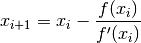
Newton’s method converges quadratically for single roots, and linearly for multiple roots.
-
gsl_root_fdfsolver_type *gsl_root_fdfsolver_secant
The secant method is a simplified version of Newton’s method which does not require the computation of the derivative on every step.
On its first iteration the algorithm begins with Newton’s method, using the derivative to compute a first step,
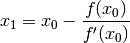
Subsequent iterations avoid the evaluation of the derivative by replacing it with a numerical estimate, the slope of the line through the previous two points,
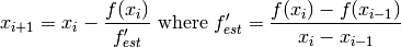
When the derivative does not change significantly in the vicinity of the root the secant method gives a useful saving. Asymptotically the secant method is faster than Newton’s method whenever the cost of evaluating the derivative is more than 0.44 times the cost of evaluating the function itself. As with all methods of computing a numerical derivative the estimate can suffer from cancellation errors if the separation of the points becomes too small.
On single roots, the method has a convergence of order
 (approximately
  ). It converges linearly for multiple
roots.
). It converges linearly for multiple
roots.
-
gsl_root_fdfsolver_type *gsl_root_fdfsolver_steffenson
The Steffenson Method 1 provides the fastest convergence of all the routines. It combines the basic Newton algorithm with an Aitken “delta-squared” acceleration. If the Newton iterates are
 then the acceleration procedure
generates a new sequence
then the acceleration procedure
generates a new sequence  ,
,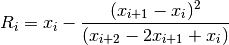
which converges faster than the original sequence under reasonable conditions. The new sequence requires three terms before it can produce its first value so the method returns accelerated values on the second and subsequent iterations. On the first iteration it returns the ordinary Newton estimate. The Newton iterate is also returned if the denominator of the acceleration term ever becomes zero.
As with all acceleration procedures this method can become unstable if the function is not well-behaved.
-
gsl_root_fdfsolver_type *gsl_root_fdfsolver_newton
Examples
For any root finding algorithm we need to prepare the function to be
solved. For this example we will use the general quadratic equation
described earlier. We first need a header file (demo_fn.h) to
define the function parameters,
struct quadratic_params
  {
    double a, b, c;
  };

double quadratic (double x, void *params);
double quadratic_deriv (double x, void *params);
void quadratic_fdf (double x, void *params,
                    double *y, double *dy);
We place the function definitions in a separate file (demo_fn.c),
double
quadratic (double x, void *params)
{
  struct quadratic_params *p
    = (struct quadratic_params *) params;

  double a = p->a;
  double b = p->b;
  double c = p->c;

  return (a * x + b) * x + c;
}

double
quadratic_deriv (double x, void *params)
{
  struct quadratic_params *p
    = (struct quadratic_params *) params;

  double a = p->a;
  double b = p->b;

  return 2.0 * a * x + b;
}

void
quadratic_fdf (double x, void *params,
               double *y, double *dy)
{
  struct quadratic_params *p
    = (struct quadratic_params *) params;

  double a = p->a;
  double b = p->b;
  double c = p->c;

  *y = (a * x + b) * x + c;
  *dy = 2.0 * a * x + b;
}
The first program uses the function solver gsl_root_fsolver_brent
for Brent’s method and the general quadratic defined above to solve the
following equation,

with solution 
#include <stdio.h>
#include <gsl/gsl_errno.h>
#include <gsl/gsl_math.h>
#include <gsl/gsl_roots.h>
#include "demo_fn.h"
#include "demo_fn.c"
int
main (void)
{
int status;
int iter = 0, max_iter = 100;
const gsl_root_fsolver_type *T;
gsl_root_fsolver *s;
double r = 0, r_expected = sqrt (5.0);
double x_lo = 0.0, x_hi = 5.0;
gsl_function F;
struct quadratic_params params = {1.0, 0.0, -5.0};
F.function = &quadratic;
F.params = ¶ms;
T = gsl_root_fsolver_brent;
s = gsl_root_fsolver_alloc (T);
gsl_root_fsolver_set (s, &F, x_lo, x_hi);
printf ("using %s method\n",
gsl_root_fsolver_name (s));
printf ("%5s [%9s, %9s] %9s %10s %9s\n",
"iter", "lower", "upper", "root",
"err", "err(est)");
do
{
iter++;
status = gsl_root_fsolver_iterate (s);
r = gsl_root_fsolver_root (s);
x_lo = gsl_root_fsolver_x_lower (s);
x_hi = gsl_root_fsolver_x_upper (s);
status = gsl_root_test_interval (x_lo, x_hi,
0, 0.001);
if (status == GSL_SUCCESS)
printf ("Converged:\n");
printf ("%5d [%.7f, %.7f] %.7f %+.7f %.7f\n",
iter, x_lo, x_hi,
r, r - r_expected,
x_hi - x_lo);
}
while (status == GSL_CONTINUE && iter < max_iter);
gsl_root_fsolver_free (s);
return status;
}
Here are the results of the iterations:
$ ./a.out
using brent method
 iter [    lower,     upper]      root        err  err(est)
    1 [1.0000000, 5.0000000] 1.0000000 -1.2360680 4.0000000
    2 [1.0000000, 3.0000000] 3.0000000 +0.7639320 2.0000000
    3 [2.0000000, 3.0000000] 2.0000000 -0.2360680 1.0000000
    4 [2.2000000, 3.0000000] 2.2000000 -0.0360680 0.8000000
    5 [2.2000000, 2.2366300] 2.2366300 +0.0005621 0.0366300
Converged:
    6 [2.2360634, 2.2366300] 2.2360634 -0.0000046 0.0005666
If the program is modified to use the bisection solver instead of
Brent’s method, by changing gsl_root_fsolver_brent to
gsl_root_fsolver_bisection the slower convergence of the
Bisection method can be observed:
$ ./a.out
using bisection method
 iter [    lower,     upper]      root        err  err(est)
    1 [0.0000000, 2.5000000] 1.2500000 -0.9860680 2.5000000
    2 [1.2500000, 2.5000000] 1.8750000 -0.3610680 1.2500000
    3 [1.8750000, 2.5000000] 2.1875000 -0.0485680 0.6250000
    4 [2.1875000, 2.5000000] 2.3437500 +0.1076820 0.3125000
    5 [2.1875000, 2.3437500] 2.2656250 +0.0295570 0.1562500
    6 [2.1875000, 2.2656250] 2.2265625 -0.0095055 0.0781250
    7 [2.2265625, 2.2656250] 2.2460938 +0.0100258 0.0390625
    8 [2.2265625, 2.2460938] 2.2363281 +0.0002601 0.0195312
    9 [2.2265625, 2.2363281] 2.2314453 -0.0046227 0.0097656
   10 [2.2314453, 2.2363281] 2.2338867 -0.0021813 0.0048828
   11 [2.2338867, 2.2363281] 2.2351074 -0.0009606 0.0024414
Converged:
   12 [2.2351074, 2.2363281] 2.2357178 -0.0003502 0.0012207
The next program solves the same function using a derivative solver instead.
#include <stdio.h>
#include <gsl/gsl_errno.h>
#include <gsl/gsl_math.h>
#include <gsl/gsl_roots.h>
#include "demo_fn.h"
#include "demo_fn.c"
int
main (void)
{
int status;
int iter = 0, max_iter = 100;
const gsl_root_fdfsolver_type *T;
gsl_root_fdfsolver *s;
double x0, x = 5.0, r_expected = sqrt (5.0);
gsl_function_fdf FDF;
struct quadratic_params params = {1.0, 0.0, -5.0};
FDF.f = &quadratic;
FDF.df = &quadratic_deriv;
FDF.fdf = &quadratic_fdf;
FDF.params = ¶ms;
T = gsl_root_fdfsolver_newton;
s = gsl_root_fdfsolver_alloc (T);
gsl_root_fdfsolver_set (s, &FDF, x);
printf ("using %s method\n",
gsl_root_fdfsolver_name (s));
printf ("%-5s %10s %10s %10s\n",
"iter", "root", "err", "err(est)");
do
{
iter++;
status = gsl_root_fdfsolver_iterate (s);
x0 = x;
x = gsl_root_fdfsolver_root (s);
status = gsl_root_test_delta (x, x0, 0, 1e-3);
if (status == GSL_SUCCESS)
printf ("Converged:\n");
printf ("%5d %10.7f %+10.7f %10.7f\n",
iter, x, x - r_expected, x - x0);
}
while (status == GSL_CONTINUE && iter < max_iter);
gsl_root_fdfsolver_free (s);
return status;
}
Here are the results for Newton’s method:
$ ./a.out
using newton method
iter        root        err   err(est)
    1  3.0000000 +0.7639320 -2.0000000
    2  2.3333333 +0.0972654 -0.6666667
    3  2.2380952 +0.0020273 -0.0952381
Converged:
    4  2.2360689 +0.0000009 -0.0020263
Note that the error can be estimated more accurately by taking the
difference between the current iterate and next iterate rather than the
previous iterate. The other derivative solvers can be investigated by
changing gsl_root_fdfsolver_newton to
gsl_root_fdfsolver_secant or
gsl_root_fdfsolver_steffenson.
References and Further Reading
For information on the Brent-Dekker algorithm see the following two papers,
R. P. Brent, “An algorithm with guaranteed convergence for finding a zero of a function”, Computer Journal, 14 (1971) 422–425
J. C. P. Bus and T. J. Dekker, “Two Efficient Algorithms with Guaranteed Convergence for Finding a Zero of a Function”, ACM Transactions of Mathematical Software, Vol.: 1 No.: 4 (1975) 330–345
Footnotes
- 1
J.F. Steffensen (1873–1961). The spelling used in the name of the function is slightly incorrect, but has been preserved to avoid incompatibility.