Simulated Annealing
Stochastic search techniques are used when the structure of a space is not well understood or is not smooth, so that techniques like Newton’s method (which requires calculating Jacobian derivative matrices) cannot be used. In particular, these techniques are frequently used to solve combinatorial optimization problems, such as the traveling salesman problem.
The goal is to find a point in the space at which a real valued energy function (or cost function) is minimized. Simulated annealing is a minimization technique which has given good results in avoiding local minima; it is based on the idea of taking a random walk through the space at successively lower temperatures, where the probability of taking a step is given by a Boltzmann distribution.
The functions described in this chapter are declared in the header file
gsl_siman.h.
Simulated Annealing algorithm
The simulated annealing algorithm takes random walks through the problem space, looking for points with low energies; in these random walks, the probability of taking a step is determined by the Boltzmann distribution,
if
 , and
, and
 when
when
 .
.
In other words, a step will occur if the new energy is lower. If
the new energy is higher, the transition can still occur, and its
likelihood is proportional to the temperature  and inversely
proportional to the energy difference
and inversely
proportional to the energy difference
 .
.
The temperature is initially set to a high value, and a random
walk is carried out at that temperature. Then the temperature is
lowered very slightly according to a cooling schedule, for
example:  where
where  is slightly greater than 1.
The slight probability of taking a step that gives higher energy is what allows simulated annealing to frequently get out of local minima.
Simulated Annealing functions
-
void gsl_siman_solve(const gsl_rng *r, void *x0_p, gsl_siman_Efunc_t Ef, gsl_siman_step_t take_step, gsl_siman_metric_t distance, gsl_siman_print_t print_position, gsl_siman_copy_t copyfunc, gsl_siman_copy_construct_t copy_constructor, gsl_siman_destroy_t destructor, size_t element_size, gsl_siman_params_t params)
This function performs a simulated annealing search through a given space. The space is specified by providing the functions
Efanddistance. The simulated annealing steps are generated using the random number generatorrand the functiontake_step.The starting configuration of the system should be given by
x0_p. The routine offers two modes for updating configurations, a fixed-size mode and a variable-size mode. In the fixed-size mode the configuration is stored as a single block of memory of sizeelement_size. Copies of this configuration are created, copied and destroyed internally using the standard library functionsmalloc(),memcpy()andfree(). The function pointerscopyfunc,copy_constructoranddestructorshould be null pointers in fixed-size mode. In the variable-size mode the functionscopyfunc,copy_constructoranddestructorare used to create, copy and destroy configurations internally. The variableelement_sizeshould be zero in the variable-size mode.The
paramsstructure (described below) controls the run by providing the temperature schedule and other tunable parameters to the algorithm.On exit the best result achieved during the search is placed in
x0_p. If the annealing process has been successful this should be a good approximation to the optimal point in the space.If the function pointer
print_positionis not null, a debugging log will be printed tostdoutwith the following columns:#-iter #-evals temperature position energy best_energyand the output of the function
print_positionitself. Ifprint_positionis null then no information is printed.
The simulated annealing routines require several user-specified functions to define the configuration space and energy function. The prototypes for these functions are given below.
-
type gsl_siman_Efunc_t
This function type should return the energy of a configuration
xp:double (*gsl_siman_Efunc_t) (void *xp)
-
type gsl_siman_step_t
This function type should modify the configuration
xpusing a random step taken from the generatorr, up to a maximum distance ofstep_size:void (*gsl_siman_step_t) (const gsl_rng *r, void *xp, double step_size)
-
type gsl_siman_metric_t
This function type should return the distance between two configurations
xpandyp:double (*gsl_siman_metric_t) (void *xp, void *yp)
-
type gsl_siman_print_t
This function type should print the contents of the configuration
xp:void (*gsl_siman_print_t) (void *xp)
-
type gsl_siman_copy_t
This function type should copy the configuration
sourceintodest:void (*gsl_siman_copy_t) (void *source, void *dest)
-
type gsl_siman_copy_construct_t
This function type should create a new copy of the configuration
xp:void * (*gsl_siman_copy_construct_t) (void *xp)
-
type gsl_siman_destroy_t
This function type should destroy the configuration
xp, freeing its memory:void (*gsl_siman_destroy_t) (void *xp)
-
type gsl_siman_params_t
These are the parameters that control a run of
gsl_siman_solve(). This structure contains all the information needed to control the search, beyond the energy function, the step function and the initial guess.int n_triesThe number of points to try for each step.
int iters_fixed_TThe number of iterations at each temperature.
double step_sizeThe maximum step size in the random walk.
double k, t_initial, mu_t, t_minThe parameters of the Boltzmann distribution and cooling schedule.
Examples
The simulated annealing package is clumsy, and it has to be because it is written in C, for C callers, and tries to be polymorphic at the same time. But here we provide some examples which can be pasted into your application with little change and should make things easier.
Trivial example
The first example, in one dimensional Cartesian space, sets up an energy function which is a damped sine wave; this has many local minima, but only one global minimum, somewhere between 1.0 and 1.5. The initial guess given is 15.5, which is several local minima away from the global minimum.
#include <math.h>
#include <stdlib.h>
#include <string.h>
#include <gsl/gsl_siman.h>

/* set up parameters for this simulated annealing run */

/* how many points do we try before stepping */
#define N_TRIES 200

/* how many iterations for each T? */
#define ITERS_FIXED_T 1000

/* max step size in random walk */
#define STEP_SIZE 1.0

/* Boltzmann constant */
#define K 1.0

/* initial temperature */
#define T_INITIAL 0.008

/* damping factor for temperature */
#define MU_T 1.003
#define T_MIN 2.0e-6

gsl_siman_params_t params
  = {N_TRIES, ITERS_FIXED_T, STEP_SIZE,
     K, T_INITIAL, MU_T, T_MIN};

/* now some functions to test in one dimension */
double E1(void *xp)
{
  double x = * ((double *) xp);

  return exp(-pow((x-1.0),2.0))*sin(8*x);
}

double M1(void *xp, void *yp)
{
  double x = *((double *) xp);
  double y = *((double *) yp);

  return fabs(x - y);
}

void S1(const gsl_rng * r, void *xp, double step_size)
{
  double old_x = *((double *) xp);
  double new_x;

  double u = gsl_rng_uniform(r);
  new_x = u * 2 * step_size - step_size + old_x;

  memcpy(xp, &new_x, sizeof(new_x));
}

void P1(void *xp)
{
  printf ("%12g", *((double *) xp));
}

int
main(void)
{
  const gsl_rng_type * T;
  gsl_rng * r;

  double x_initial = 15.5;

  gsl_rng_env_setup();

  T = gsl_rng_default;
  r = gsl_rng_alloc(T);

  gsl_siman_solve(r, &x_initial, E1, S1, M1, P1,
                  NULL, NULL, NULL,
                  sizeof(double), params);

  gsl_rng_free (r);
  return 0;
}
Fig. 16 is generated by running
siman_test in the following way:
$ ./siman_test | awk '!/^#/ {print $1, $4}'
 | graph -y 1.34 1.4 -W0 -X generation -Y position
 | plot -Tps > siman-test.eps
Fig. 17 is generated by running
siman_test in the following way:
$ ./siman_test | awk '!/^#/ {print $1, $5}'
 | graph -y -0.88 -0.83 -W0 -X generation -Y energy
 | plot -Tps > siman-energy.eps
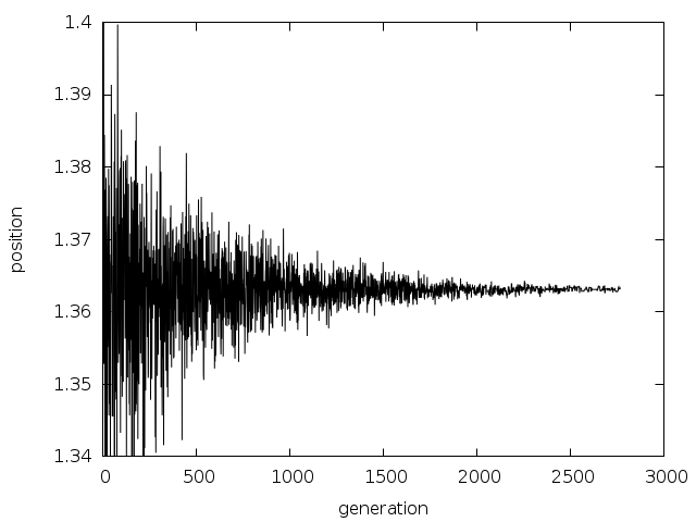
Fig. 16 Example of a simulated annealing run: at higher temperatures (early in the plot) you see that the solution can fluctuate, but at lower temperatures it converges.
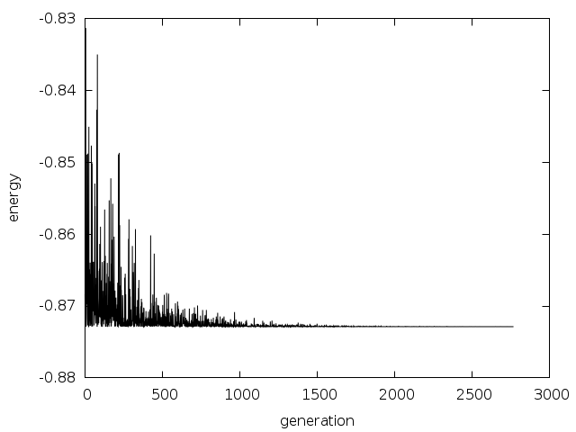
Fig. 17 Simulated annealing energy vs generation
Traveling Salesman Problem
The TSP (Traveling Salesman Problem) is the classic combinatorial optimization problem. I have provided a very simple version of it, based on the coordinates of twelve cities in the southwestern United States. This should maybe be called the Flying Salesman Problem, since I am using the great-circle distance between cities, rather than the driving distance. Also: I assume the earth is a sphere, so I don’t use geoid distances.
The gsl_siman_solve() routine finds a route which is 3490.62
Kilometers long; this is confirmed by an exhaustive search of all
possible routes with the same initial city.
The full code is given below.
/* siman/siman_tsp.c
 *
 * Copyright (C) 1996, 1997, 1998, 1999, 2000 Mark Galassi
 *
 * This program is free software; you can redistribute it and/or modify
 * it under the terms of the GNU General Public License as published by
 * the Free Software Foundation; either version 3 of the License, or (at
 * your option) any later version.
 *
 * This program is distributed in the hope that it will be useful, but
 * WITHOUT ANY WARRANTY; without even the implied warranty of
 * MERCHANTABILITY or FITNESS FOR A PARTICULAR PURPOSE.  See the GNU
 * General Public License for more details.
 *
 * You should have received a copy of the GNU General Public License
 * along with this program; if not, write to the Free Software
 * Foundation, Inc., 51 Franklin Street, Fifth Floor, Boston, MA 02110-1301, USA.
 */

#include <config.h>
#include <math.h>
#include <string.h>
#include <stdio.h>
#include <gsl/gsl_math.h>
#include <gsl/gsl_rng.h>
#include <gsl/gsl_siman.h>
#include <gsl/gsl_ieee_utils.h>

/* set up parameters for this simulated annealing run */

#define N_TRIES 200             /* how many points do we try before stepping */
#define ITERS_FIXED_T 2000      /* how many iterations for each T? */
#define STEP_SIZE 1.0           /* max step size in random walk */
#define K 1.0                   /* Boltzmann constant */
#define T_INITIAL 5000.0        /* initial temperature */
#define MU_T 1.002              /* damping factor for temperature */
#define T_MIN 5.0e-1

gsl_siman_params_t params = {N_TRIES, ITERS_FIXED_T, STEP_SIZE,
                             K, T_INITIAL, MU_T, T_MIN};

struct s_tsp_city {
  const char * name;
  double lat, longitude;        /* coordinates */
};
typedef struct s_tsp_city Stsp_city;

void prepare_distance_matrix(void);
void exhaustive_search(void);
void print_distance_matrix(void);
double city_distance(Stsp_city c1, Stsp_city c2);
double Etsp(void *xp);
double Mtsp(void *xp, void *yp);
void Stsp(const gsl_rng * r, void *xp, double step_size);
void Ptsp(void *xp);

/* in this table, latitude and longitude are obtained from the US
   Census Bureau, at http://www.census.gov/cgi-bin/gazetteer */

Stsp_city cities[] = {{"Santa Fe",    35.68,   105.95},
                      {"Phoenix",     33.54,   112.07},
                      {"Albuquerque", 35.12,   106.62},
                      {"Clovis",      34.41,   103.20},
                      {"Durango",     37.29,   107.87},
                      {"Dallas",      32.79,    96.77},
                      {"Tesuque",     35.77,   105.92},
                      {"Grants",      35.15,   107.84},
                      {"Los Alamos",  35.89,   106.28},
                      {"Las Cruces",  32.34,   106.76},
                      {"Cortez",      37.35,   108.58},
                      {"Gallup",      35.52,   108.74}};

#define N_CITIES (sizeof(cities)/sizeof(Stsp_city))

double distance_matrix[N_CITIES][N_CITIES];

/* distance between two cities */
double city_distance(Stsp_city c1, Stsp_city c2)
{
  const double earth_radius = 6375.000; /* 6000KM approximately */
  /* sin and cos of lat and long; must convert to radians */
  double sla1 = sin(c1.lat*M_PI/180), cla1 = cos(c1.lat*M_PI/180),
    slo1 = sin(c1.longitude*M_PI/180), clo1 = cos(c1.longitude*M_PI/180);
  double sla2 = sin(c2.lat*M_PI/180), cla2 = cos(c2.lat*M_PI/180),
    slo2 = sin(c2.longitude*M_PI/180), clo2 = cos(c2.longitude*M_PI/180);

  double x1 = cla1*clo1;
  double x2 = cla2*clo2;

  double y1 = cla1*slo1;
  double y2 = cla2*slo2;

  double z1 = sla1;
  double z2 = sla2;

  double dot_product = x1*x2 + y1*y2 + z1*z2;

  double angle = acos(dot_product);

  /* distance is the angle (in radians) times the earth radius */
  return angle*earth_radius;
}

/* energy for the travelling salesman problem */
double Etsp(void *xp)
{
  /* an array of N_CITIES integers describing the order */
  int *route = (int *) xp;
  double E = 0;
  unsigned int i;

  for (i = 0; i < N_CITIES; ++i) {
    /* use the distance_matrix to optimize this calculation; it had
       better be allocated!! */
    E += distance_matrix[route[i]][route[(i + 1) % N_CITIES]];
  }

  return E;
}

double Mtsp(void *xp, void *yp)
{
  int *route1 = (int *) xp, *route2 = (int *) yp;
  double distance = 0;
  unsigned int i;

  for (i = 0; i < N_CITIES; ++i) {
    distance += ((route1[i] == route2[i]) ? 0 : 1);
  }

  return distance;
}

/* take a step through the TSP space */
void Stsp(const gsl_rng * r, void *xp, double step_size)
{
  int x1, x2, dummy;
  int *route = (int *) xp;

  step_size = 0 ; /* prevent warnings about unused parameter */

  /* pick the two cities to swap in the matrix; we leave the first
     city fixed */
  x1 = (gsl_rng_get (r) % (N_CITIES-1)) + 1;
  do {
    x2 = (gsl_rng_get (r) % (N_CITIES-1)) + 1;
  } while (x2 == x1);

  dummy = route[x1];
  route[x1] = route[x2];
  route[x2] = dummy;
}

void Ptsp(void *xp)
{
  unsigned int i;
  int *route = (int *) xp;
  printf("  [");
  for (i = 0; i < N_CITIES; ++i) {
    printf(" %d ", route[i]);
  }
  printf("]  ");
}

int main(void)
{
  int x_initial[N_CITIES];
  unsigned int i;

  const gsl_rng * r = gsl_rng_alloc (gsl_rng_env_setup()) ;

  gsl_ieee_env_setup ();

  prepare_distance_matrix();

  /* set up a trivial initial route */
  printf("# initial order of cities:\n");
  for (i = 0; i < N_CITIES; ++i) {
    printf("# \"%s\"\n", cities[i].name);
    x_initial[i] = i;
  }

  printf("# distance matrix is:\n");
  print_distance_matrix();

  printf("# initial coordinates of cities (longitude and latitude)\n");
  /* this can be plotted with */
  /* ./siman_tsp > hhh ; grep city_coord hhh | awk '{print $2 "   " $3}' | xyplot -ps -d "xy" > c.eps */
  for (i = 0; i < N_CITIES+1; ++i) {
    printf("###initial_city_coord: %g %g \"%s\"\n",
           -cities[x_initial[i % N_CITIES]].longitude,
           cities[x_initial[i % N_CITIES]].lat,
           cities[x_initial[i % N_CITIES]].name);
  }

/*   exhaustive_search(); */

  gsl_siman_solve(r, x_initial, Etsp, Stsp, Mtsp, Ptsp, NULL, NULL, NULL,
                  N_CITIES*sizeof(int), params);

  printf("# final order of cities:\n");
  for (i = 0; i < N_CITIES; ++i) {
    printf("# \"%s\"\n", cities[x_initial[i]].name);
  }

  printf("# final coordinates of cities (longitude and latitude)\n");
  /* this can be plotted with */
  /* ./siman_tsp > hhh ; grep city_coord hhh | awk '{print $2 "   " $3}' | xyplot -ps -d "xy" > c.eps */
  for (i = 0; i < N_CITIES+1; ++i) {
    printf("###final_city_coord: %g %g %s\n",
           -cities[x_initial[i % N_CITIES]].longitude,
           cities[x_initial[i % N_CITIES]].lat,
           cities[x_initial[i % N_CITIES]].name);
  }

  printf("# ");
  fflush(stdout);
#if 0
  system("date");
#endif /* 0 */
  fflush(stdout);

  return 0;
}

void prepare_distance_matrix()
{
  unsigned int i, j;
  double dist;

  for (i = 0; i < N_CITIES; ++i) {
    for (j = 0; j < N_CITIES; ++j) {
      if (i == j) {
        dist = 0;
      } else {
        dist = city_distance(cities[i], cities[j]);
      }
      distance_matrix[i][j] = dist;
    }
  }
}

void print_distance_matrix()
{
  unsigned int i, j;

  for (i = 0; i < N_CITIES; ++i) {
    printf("# ");
    for (j = 0; j < N_CITIES; ++j) {
      printf("%15.8f   ", distance_matrix[i][j]);
    }
    printf("\n");
  }
}

/* [only works for 12] search the entire space for solutions */
static double best_E = 1.0e100, second_E = 1.0e100, third_E = 1.0e100;
static int best_route[N_CITIES];
static int second_route[N_CITIES];
static int third_route[N_CITIES];
static void do_all_perms(int *route, int n);

void exhaustive_search()
{
  static int initial_route[N_CITIES] = {0, 1, 2, 3, 4, 5, 6, 7, 8, 9, 10, 11};
  printf("\n# ");
  fflush(stdout);
#if 0
  system("date");
#endif
  fflush(stdout);
  do_all_perms(initial_route, 1);
  printf("\n# ");
  fflush(stdout);
#if 0
  system("date");
#endif /* 0 */
  fflush(stdout);

  printf("# exhaustive best route: ");
  Ptsp(best_route);
  printf("\n# its energy is: %g\n", best_E);

  printf("# exhaustive second_best route: ");
  Ptsp(second_route);
  printf("\n# its energy is: %g\n", second_E);

  printf("# exhaustive third_best route: ");
  Ptsp(third_route);
  printf("\n# its energy is: %g\n", third_E);
}

/* James Theiler's recursive algorithm for generating all routes */
static void do_all_perms(int *route, int n)
{
  if (n == (N_CITIES-1)) {
    /* do it! calculate the energy/cost for that route */
    double E;
    E = Etsp(route);            /* TSP energy function */
    /* now save the best 3 energies and routes */
    if (E < best_E) {
      third_E = second_E;
      memcpy(third_route, second_route, N_CITIES*sizeof(*route));
      second_E = best_E;
      memcpy(second_route, best_route, N_CITIES*sizeof(*route));
      best_E = E;
      memcpy(best_route, route, N_CITIES*sizeof(*route));
    } else if (E < second_E) {
      third_E = second_E;
      memcpy(third_route, second_route, N_CITIES*sizeof(*route));
      second_E = E;
      memcpy(second_route, route, N_CITIES*sizeof(*route));
    } else if (E < third_E) {
      third_E = E;
      memcpy(route, third_route, N_CITIES*sizeof(*route));
    }
  } else {
    int new_route[N_CITIES];
    unsigned int j;
    int swap_tmp;
    memcpy(new_route, route, N_CITIES*sizeof(*route));
    for (j = n; j < N_CITIES; ++j) {
      swap_tmp = new_route[j];
      new_route[j] = new_route[n];
      new_route[n] = swap_tmp;
      do_all_perms(new_route, n+1);
    }
  }
}
Below are some plots generated in the following way:
$ ./siman_tsp > tsp.output
$ grep -v "^#" tsp.output
 | awk '{print $1, $NF}'
 | graph -y 3300 6500 -W0 -X generation -Y distance
    -L "TSP - 12 southwest cities"
 | plot -Tps > 12-cities.eps
$ grep initial_city_coord tsp.output
  | awk '{print $2, $3}'
  | graph -X "longitude (- means west)" -Y "latitude"
     -L "TSP - initial-order" -f 0.03 -S 1 0.1
  | plot -Tps > initial-route.eps
$ grep final_city_coord tsp.output
  | awk '{print $2, $3}'
  | graph -X "longitude (- means west)" -Y "latitude"
     -L "TSP - final-order" -f 0.03 -S 1 0.1
  | plot -Tps > final-route.eps
This is the output showing the initial order of the cities; longitude is negative, since it is west and I want the plot to look like a map:
# initial coordinates of cities (longitude and latitude)
###initial_city_coord: -105.95 35.68 Santa Fe
###initial_city_coord: -112.07 33.54 Phoenix
###initial_city_coord: -106.62 35.12 Albuquerque
###initial_city_coord: -103.2 34.41 Clovis
###initial_city_coord: -107.87 37.29 Durango
###initial_city_coord: -96.77 32.79 Dallas
###initial_city_coord: -105.92 35.77 Tesuque
###initial_city_coord: -107.84 35.15 Grants
###initial_city_coord: -106.28 35.89 Los Alamos
###initial_city_coord: -106.76 32.34 Las Cruces
###initial_city_coord: -108.58 37.35 Cortez
###initial_city_coord: -108.74 35.52 Gallup
###initial_city_coord: -105.95 35.68 Santa Fe
The optimal route turns out to be:
# final coordinates of cities (longitude and latitude)
###final_city_coord: -105.95 35.68 Santa Fe
###final_city_coord: -103.2 34.41 Clovis
###final_city_coord: -96.77 32.79 Dallas
###final_city_coord: -106.76 32.34 Las Cruces
###final_city_coord: -112.07 33.54 Phoenix
###final_city_coord: -108.74 35.52 Gallup
###final_city_coord: -108.58 37.35 Cortez
###final_city_coord: -107.87 37.29 Durango
###final_city_coord: -107.84 35.15 Grants
###final_city_coord: -106.62 35.12 Albuquerque
###final_city_coord: -106.28 35.89 Los Alamos
###final_city_coord: -105.92 35.77 Tesuque
###final_city_coord: -105.95 35.68 Santa Fe
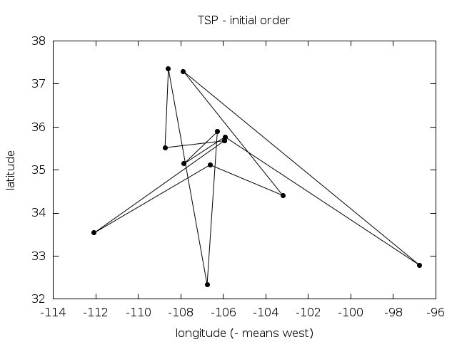
Fig. 18 Initial route for the 12 southwestern cities Flying Salesman Problem.
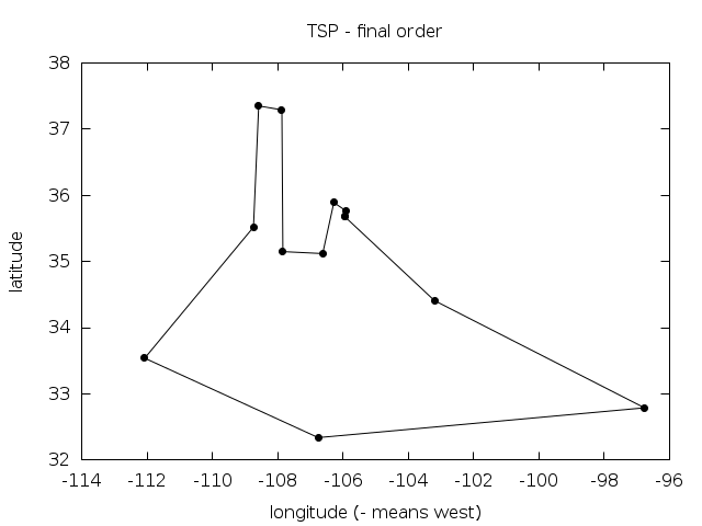
Fig. 19 Final (optimal) route for the 12 southwestern cities Flying Salesman Problem.
Here’s a plot of the cost function (energy) versus generation (point in the calculation at which a new temperature is set) for this problem:
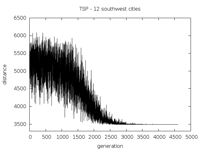
Fig. 20 Example of a simulated annealing run for the 12 southwestern cities Flying Salesman Problem.
References and Further Reading
Further information is available in the following book,
Modern Heuristic Techniques for Combinatorial Problems, Colin R. Reeves (ed.), McGraw-Hill, 1995 (ISBN 0-07-709239-2).