Fast Fourier Transforms (FFTs)
This chapter describes functions for performing Fast Fourier Transforms (FFTs). The library includes radix-2 routines (for lengths which are a power of two) and mixed-radix routines (which work for any length). For efficiency there are separate versions of the routines for real data and for complex data. The mixed-radix routines are a reimplementation of the FFTPACK library of Paul Swarztrauber. Fortran code for FFTPACK is available on Netlib (FFTPACK also includes some routines for sine and cosine transforms but these are currently not available in GSL). For details and derivations of the underlying algorithms consult the document “GSL FFT Algorithms” (see References and Further Reading)
Mathematical Definitions
Fast Fourier Transforms are efficient algorithms for calculating the discrete Fourier transform (DFT),
The DFT usually arises as an approximation to the continuous Fourier
transform when functions are sampled at discrete intervals in space or
time. The naive evaluation of the discrete Fourier transform is a
matrix-vector multiplication  .
A general matrix-vector multiplication takes
.
A general matrix-vector multiplication takes
 operations for
  data-points. Fast Fourier
transform algorithms use a divide-and-conquer strategy to factorize the
matrix
data-points. Fast Fourier
transform algorithms use a divide-and-conquer strategy to factorize the
matrix  into smaller sub-matrices, corresponding to the integer
factors of the length . If can be factorized into a
product of integers
into smaller sub-matrices, corresponding to the integer
factors of the length . If can be factorized into a
product of integers  then the DFT can be computed in
  operations. For a radix-2 FFT this gives an operation count of
 .
.
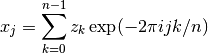
All the FFT functions offer three types of transform: forwards, inverse
and backwards, based on the same mathematical definitions. The
definition of the forward Fourier transform,
 , is,
, is,
and the definition of the inverse Fourier transform,
 , is,
, is,
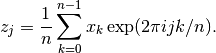
The factor of  makes this a true inverse. For example, a call
to
makes this a true inverse. For example, a call
to gsl_fft_complex_forward() followed by a call to
gsl_fft_complex_inverse() should return the original data (within
numerical errors).
In general there are two possible choices for the sign of the exponential in the transform/ inverse-transform pair. GSL follows the same convention as FFTPACK, using a negative exponential for the forward transform. The advantage of this convention is that the inverse transform recreates the original function with simple Fourier synthesis. Numerical Recipes uses the opposite convention, a positive exponential in the forward transform.
The backwards FFT is simply our terminology for an unscaled version of the inverse FFT,
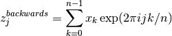
When the overall scale of the result is unimportant it is often convenient to use the backwards FFT instead of the inverse to save unnecessary divisions.
Overview of complex data FFTs
The inputs and outputs for the complex FFT routines are packed arrays of floating point numbers. In a packed array the real and imaginary parts of each complex number are placed in alternate neighboring elements. For example, the following definition of a packed array of length 6:
double x[3*2];
gsl_complex_packed_array data = x;
can be used to hold an array of three complex numbers, z[3], in
the following way:
data[0] = Re(z[0])
data[1] = Im(z[0])
data[2] = Re(z[1])
data[3] = Im(z[1])
data[4] = Re(z[2])
data[5] = Im(z[2])
The array indices for the data have the same ordering as those in the definition of the DFT—i.e. there are no index transformations or permutations of the data.
A stride parameter allows the user to perform transforms on the
elements z[stride*i] instead of z[i]. A stride greater
than 1 can be used to take an in-place FFT of the column of a matrix. A
stride of 1 accesses the array without any additional spacing between
elements.
To perform an FFT on a vector argument, such as gsl_vector_complex * v,
use the following definitions (or their equivalents) when calling
the functions described in this chapter:
gsl_complex_packed_array data = v->data;
size_t stride = v->stride;
size_t n = v->size;
For physical applications it is important to remember that the index
appearing in the DFT does not correspond directly to a physical
frequency. If the time-step of the DFT is  then the
frequency-domain includes both positive and negative frequencies,
ranging from
then the
frequency-domain includes both positive and negative frequencies,
ranging from  through 0 to
  . The
positive frequencies are stored from the beginning of the array up to
the middle, and the negative frequencies are stored backwards from the
end of the array.
. The
positive frequencies are stored from the beginning of the array up to
the middle, and the negative frequencies are stored backwards from the
end of the array.
Here is a table which shows the layout of the array data, and the
correspondence between the time-domain data  , and the
frequency-domain data
, and the
frequency-domain data  :
:
index    z               x = FFT(z)

0        z(t = 0)        x(f = 0)
1        z(t = 1)        x(f = 1/(n Delta))
2        z(t = 2)        x(f = 2/(n Delta))
.        ........        ..................
n/2      z(t = n/2)      x(f = +1/(2 Delta),
                               -1/(2 Delta))
.        ........        ..................
n-3      z(t = n-3)      x(f = -3/(n Delta))
n-2      z(t = n-2)      x(f = -2/(n Delta))
n-1      z(t = n-1)      x(f = -1/(n Delta))
When is even the location  contains the most positive
and negative frequencies (
contains the most positive
and negative frequencies ( ,
,  )
which are equivalent. If is odd then general structure of the
table above still applies, but does not appear.
)
which are equivalent. If is odd then general structure of the
table above still applies, but does not appear.
Radix-2 FFT routines for complex data
The radix-2 algorithms described in this section are simple and compact, although not necessarily the most efficient. They use the Cooley-Tukey algorithm to compute in-place complex FFTs for lengths which are a power of 2—no additional storage is required. The corresponding self-sorting mixed-radix routines offer better performance at the expense of requiring additional working space.
All the functions described in this section are declared in the header file gsl_fft_complex.h.
-
int gsl_fft_complex_radix2_forward(gsl_complex_packed_array data, size_t stride, size_t n)
-
int gsl_fft_complex_radix2_transform(gsl_complex_packed_array data, size_t stride, size_t n, gsl_fft_direction sign)
-
int gsl_fft_complex_radix2_backward(gsl_complex_packed_array data, size_t stride, size_t n)
-
int gsl_fft_complex_radix2_inverse(gsl_complex_packed_array data, size_t stride, size_t n)
These functions compute forward, backward and inverse FFTs of length
nwith stridestride, on the packed complex arraydatausing an in-place radix-2 decimation-in-time algorithm. The length of the transformnis restricted to powers of two. For thetransformversion of the function thesignargument can be eitherforward( ) or
) or backward( ).
).The functions return a value of
GSL_SUCCESSif no errors were detected, orGSL_EDOMif the length of the datanis not a power of two.
-
int gsl_fft_complex_radix2_dif_forward(gsl_complex_packed_array data, size_t stride, size_t n)
-
int gsl_fft_complex_radix2_dif_transform(gsl_complex_packed_array data, size_t stride, size_t n, gsl_fft_direction sign)
-
int gsl_fft_complex_radix2_dif_backward(gsl_complex_packed_array data, size_t stride, size_t n)
-
int gsl_fft_complex_radix2_dif_inverse(gsl_complex_packed_array data, size_t stride, size_t n)
These are decimation-in-frequency versions of the radix-2 FFT functions.
Here is an example program which computes the FFT of a short pulse in a
sample of length 128. To make the resulting Fourier transform real the
pulse is defined for equal positive and negative times ( ),
where the negative times wrap around the end of the array.
),
where the negative times wrap around the end of the array.
#include <stdio.h>
#include <math.h>
#include <gsl/gsl_errno.h>
#include <gsl/gsl_fft_complex.h>

#define REAL(z,i) ((z)[2*(i)])
#define IMAG(z,i) ((z)[2*(i)+1])

int
main (void)
{
  int i; double data[2*128];

  for (i = 0; i < 128; i++)
    {
       REAL(data,i) = 0.0; IMAG(data,i) = 0.0;
    }

  REAL(data,0) = 1.0;

  for (i = 1; i <= 10; i++)
    {
       REAL(data,i) = REAL(data,128-i) = 1.0;
    }

  for (i = 0; i < 128; i++)
    {
      printf ("%d %e %e\n", i,
              REAL(data,i), IMAG(data,i));
    }
  printf ("\n\n");

  gsl_fft_complex_radix2_forward (data, 1, 128);

  for (i = 0; i < 128; i++)
    {
      printf ("%d %e %e\n", i,
              REAL(data,i)/sqrt(128),
              IMAG(data,i)/sqrt(128));
    }

  return 0;
}
Note that we have assumed that the program is using the default error
handler (which calls abort() for any errors). If you are not using
a safe error handler you would need to check the return status of
gsl_fft_complex_radix2_forward().
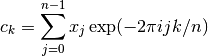
The transformed data is rescaled by  so that it fits on
the same plot as the input. Only the real part is shown, by the choice
of the input data the imaginary part is zero. Allowing for the
wrap-around of negative times at
so that it fits on
the same plot as the input. Only the real part is shown, by the choice
of the input data the imaginary part is zero. Allowing for the
wrap-around of negative times at  , and working in units of
 , the DFT approximates the continuum Fourier transform, giving
a modulated sine function.
, the DFT approximates the continuum Fourier transform, giving
a modulated sine function.
The output of the example program is plotted in Fig. 2.
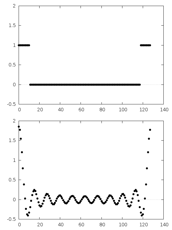
Fig. 2 A pulse and its discrete Fourier transform, output from the example program.
Mixed-radix FFT routines for complex data
This section describes mixed-radix FFT algorithms for complex data. The mixed-radix functions work for FFTs of any length. They are a reimplementation of Paul Swarztrauber’s Fortran FFTPACK library. The theory is explained in the review article “Self-sorting Mixed-radix FFTs” by Clive Temperton. The routines here use the same indexing scheme and basic algorithms as FFTPACK.
The mixed-radix algorithm is based on sub-transform modules—highly
optimized small length FFTs which are combined to create larger FFTs.
There are efficient modules for factors of 2, 3, 4, 5, 6 and 7. The
modules for the composite factors of 4 and 6 are faster than combining
the modules for  and
and  .
.
For factors which are not implemented as modules there is a fall-back to
a general length- module which uses Singleton’s method for
efficiently computing a DFT. This module is , and slower
than a dedicated module would be but works for any length . Of
course, lengths which use the general length- module will still
be factorized as much as possible. For example, a length of 143 will be
factorized into  . Large prime factors are the worst case
scenario, e.g. as found in
. Large prime factors are the worst case
scenario, e.g. as found in  , and should be avoided
because their scaling will dominate the run-time (consult
the document “GSL FFT Algorithms” included in the GSL distribution
if you encounter this problem).
, and should be avoided
because their scaling will dominate the run-time (consult
the document “GSL FFT Algorithms” included in the GSL distribution
if you encounter this problem).
The mixed-radix initialization function gsl_fft_complex_wavetable_alloc()
returns the list of factors chosen by the library for a given length
. It can be used to check how well the length has been
factorized, and estimate the run-time. To a first approximation the
run-time scales as  , where the
  are the
factors of . For programs under user control you may wish to
issue a warning that the transform will be slow when the length is
poorly factorized. If you frequently encounter data lengths which
cannot be factorized using the existing small-prime modules consult
“GSL FFT Algorithms” for details on adding support for other
factors.
are the
factors of . For programs under user control you may wish to
issue a warning that the transform will be slow when the length is
poorly factorized. If you frequently encounter data lengths which
cannot be factorized using the existing small-prime modules consult
“GSL FFT Algorithms” for details on adding support for other
factors.
All the functions described in this section are declared in the header
file gsl_fft_complex.h.
-
gsl_fft_complex_wavetable *gsl_fft_complex_wavetable_alloc(size_t n)
This function prepares a trigonometric lookup table for a complex FFT of length
n. The function returns a pointer to the newly allocatedgsl_fft_complex_wavetableif no errors were detected, and a null pointer in the case of error. The lengthnis factorized into a product of subtransforms, and the factors and their trigonometric coefficients are stored in the wavetable. The trigonometric coefficients are computed using direct calls tosinandcos, for accuracy. Recursion relations could be used to compute the lookup table faster, but if an application performs many FFTs of the same length then this computation is a one-off overhead which does not affect the final throughput.The wavetable structure can be used repeatedly for any transform of the same length. The table is not modified by calls to any of the other FFT functions. The same wavetable can be used for both forward and backward (or inverse) transforms of a given length.
-
void gsl_fft_complex_wavetable_free(gsl_fft_complex_wavetable *wavetable)
This function frees the memory associated with the wavetable
wavetable. The wavetable can be freed if no further FFTs of the same length will be needed.
These functions operate on a gsl_fft_complex_wavetable structure
which contains internal parameters for the FFT. It is not necessary to
set any of the components directly but it can sometimes be useful to
examine them. For example, the chosen factorization of the FFT length
is given and can be used to provide an estimate of the run-time or
numerical error. The wavetable structure is declared in the header file
gsl_fft_complex.h.
-
type gsl_fft_complex_wavetable
This is a structure that holds the factorization and trigonometric lookup tables for the mixed radix fft algorithm. It has the following components:
size_t nThis is the number of complex data points
size_t nfThis is the number of factors that the length
nwas decomposed into.size_t factor[64]This is the array of factors. Only the first
nfelements are used.gsl_complex * trigThis is a pointer to a preallocated trigonometric lookup table of
ncomplex elements.gsl_complex * twiddle[64]This is an array of pointers into
trig, giving the twiddle factors for each pass.
-
type gsl_fft_complex_workspace
The mixed radix algorithms require additional working space to hold the intermediate steps of the transform.
-
gsl_fft_complex_workspace *gsl_fft_complex_workspace_alloc(size_t n)
This function allocates a workspace for a complex transform of length
n.
-
void gsl_fft_complex_workspace_free(gsl_fft_complex_workspace *workspace)
This function frees the memory associated with the workspace
workspace. The workspace can be freed if no further FFTs of the same length will be needed.
The following functions compute the transform,
-
int gsl_fft_complex_forward(gsl_complex_packed_array data, size_t stride, size_t n, const gsl_fft_complex_wavetable *wavetable, gsl_fft_complex_workspace *work)
-
int gsl_fft_complex_transform(gsl_complex_packed_array data, size_t stride, size_t n, const gsl_fft_complex_wavetable *wavetable, gsl_fft_complex_workspace *work, gsl_fft_direction sign)
-
int gsl_fft_complex_backward(gsl_complex_packed_array data, size_t stride, size_t n, const gsl_fft_complex_wavetable *wavetable, gsl_fft_complex_workspace *work)
-
int gsl_fft_complex_inverse(gsl_complex_packed_array data, size_t stride, size_t n, const gsl_fft_complex_wavetable *wavetable, gsl_fft_complex_workspace *work)
These functions compute forward, backward and inverse FFTs of length
nwith stridestride, on the packed complex arraydata, using a mixed radix decimation-in-frequency algorithm. There is no restriction on the lengthn. Efficient modules are provided for subtransforms of length 2, 3, 4, 5, 6 and 7. Any remaining factors are computed with a slow,, general-
module. The caller must supply a wavetablecontaining the trigonometric lookup tables and a workspacework. For thetransformversion of the function thesignargument can be eitherforward() or backward().The functions return a value of
0if no errors were detected. The followinggsl_errnoconditions are defined for these functions:The length of the data
nis not a positive integer (i.e.nis zero).The length of the data
nand the length used to compute the givenwavetabledo not match.
Here is an example program which computes the FFT of a short pulse in a
sample of length 630 ( ) using the mixed-radix
algorithm.
) using the mixed-radix
algorithm.
#include <stdio.h>
#include <math.h>
#include <gsl/gsl_errno.h>
#include <gsl/gsl_fft_complex.h>

#define REAL(z,i) ((z)[2*(i)])
#define IMAG(z,i) ((z)[2*(i)+1])

int
main (void)
{
  int i;
  const int n = 630;
  double data[2*n];

  gsl_fft_complex_wavetable * wavetable;
  gsl_fft_complex_workspace * workspace;

  for (i = 0; i < n; i++)
    {
      REAL(data,i) = 0.0;
      IMAG(data,i) = 0.0;
    }

  data[0] = 1.0;

  for (i = 1; i <= 10; i++)
    {
      REAL(data,i) = REAL(data,n-i) = 1.0;
    }

  for (i = 0; i < n; i++)
    {
      printf ("%d: %e %e\n", i, REAL(data,i),
                                IMAG(data,i));
    }
  printf ("\n");

  wavetable = gsl_fft_complex_wavetable_alloc (n);
  workspace = gsl_fft_complex_workspace_alloc (n);

  for (i = 0; i < (int) wavetable->nf; i++)
    {
       printf ("# factor %d: %zu\n", i,
               wavetable->factor[i]);
    }

  gsl_fft_complex_forward (data, 1, n,
                           wavetable, workspace);

  for (i = 0; i < n; i++)
    {
      printf ("%d: %e %e\n", i, REAL(data,i),
                                IMAG(data,i));
    }

  gsl_fft_complex_wavetable_free (wavetable);
  gsl_fft_complex_workspace_free (workspace);
  return 0;
}
Note that we have assumed that the program is using the default
gsl error handler (which calls abort() for any errors). If
you are not using a safe error handler you would need to check the
return status of all the gsl routines.
Overview of real data FFTs
The functions for real data are similar to those for complex data. However, there is an important difference between forward and inverse transforms. The Fourier transform of a real sequence is not real. It is a complex sequence with a special symmetry:

A sequence with this symmetry is called conjugate-complex or
half-complex. This different structure requires different
storage layouts for the forward transform (from real to half-complex)
and inverse transform (from half-complex back to real). As a
consequence the routines are divided into two sets: functions in
gsl_fft_real which operate on real sequences and functions in
gsl_fft_halfcomplex which operate on half-complex sequences.
Functions in gsl_fft_real compute the frequency coefficients of a
real sequence. The half-complex coefficients  of a real sequence
are given by Fourier analysis,
of a real sequence
are given by Fourier analysis,
Functions in gsl_fft_halfcomplex compute inverse or backwards
transforms. They reconstruct real sequences by Fourier synthesis from
their half-complex frequency coefficients, ,
The symmetry of the half-complex sequence implies that only half of the
complex numbers in the output need to be stored. The remaining half can
be reconstructed using the half-complex symmetry condition. This works
for all lengths, even and odd—when the length is even the middle value
where  is also real. Thus only
 n real numbers are
required to store the half-complex sequence, and the transform of a real
sequence can be stored in the same size array as the original data.
The precise storage arrangements depend on the algorithm, and are different for radix-2 and mixed-radix routines. The radix-2 function operates in-place, which constrains the locations where each element can be stored. The restriction forces real and imaginary parts to be stored far apart. The mixed-radix algorithm does not have this restriction, and it stores the real and imaginary parts of a given term in neighboring locations (which is desirable for better locality of memory accesses).
Radix-2 FFT routines for real data
This section describes radix-2 FFT algorithms for real data. They use the Cooley-Tukey algorithm to compute in-place FFTs for lengths which are a power of 2.
The radix-2 FFT functions for real data are declared in the header files
gsl_fft_real.h
-
int gsl_fft_real_radix2_transform(double data[], size_t stride, size_t n)
This function computes an in-place radix-2 FFT of length
nand stridestrideon the real arraydata. The output is a half-complex sequence, which is stored in-place. The arrangement of the half-complex terms uses the following scheme: for the
real part of the
the
real part of the  -th term is stored in location , and
the corresponding imaginary part is stored in location
-th term is stored in location , and
the corresponding imaginary part is stored in location  . Terms
with
. Terms
with  can be reconstructed using the symmetry
 .
The terms for
.
The terms for  and are both purely
real, and count as a special case. Their real parts are stored in
locations
and are both purely
real, and count as a special case. Their real parts are stored in
locations  and respectively, while their imaginary
parts which are zero are not stored.
and respectively, while their imaginary
parts which are zero are not stored.The following table shows the correspondence between the output
dataand the equivalent results obtained by considering the input data as a complex sequence with zero imaginary part (assumingstride= 1}):complex[0].real = data[0] complex[0].imag = 0 complex[1].real = data[1] complex[1].imag = data[n-1] ............... ................ complex[k].real = data[k] complex[k].imag = data[n-k] ............... ................ complex[n/2].real = data[n/2] complex[n/2].imag = 0 ............... ................ complex[k'].real = data[k] k' = n - k complex[k'].imag = -data[n-k] ............... ................ complex[n-1].real = data[1] complex[n-1].imag = -data[n-1]
Note that the output data can be converted into the full complex sequence using the function
gsl_fft_halfcomplex_radix2_unpack()described below.
The radix-2 FFT functions for halfcomplex data are declared in the
header file gsl_fft_halfcomplex.h.
-
int gsl_fft_halfcomplex_radix2_inverse(double data[], size_t stride, size_t n)
-
int gsl_fft_halfcomplex_radix2_backward(double data[], size_t stride, size_t n)
These functions compute the inverse or backwards in-place radix-2 FFT of length
nand stridestrideon the half-complex sequencedatastored according the output scheme used bygsl_fft_real_radix2(). The result is a real array stored in natural order.
-
int gsl_fft_halfcomplex_radix2_unpack(const double halfcomplex_coefficient[], gsl_complex_packed_array complex_coefficient, size_t stride, size_t n)
This function converts
halfcomplex_coefficient, an array of half-complex coefficients as returned bygsl_fft_real_radix2_transform(), into an ordinary complex array,complex_coefficient. It fills in the complex array using the symmetry to reconstruct the redundant elements. The algorithm for the conversion
is:
to reconstruct the redundant elements. The algorithm for the conversion
is:complex_coefficient[0].real = halfcomplex_coefficient[0]; complex_coefficient[0].imag = 0.0; for (i = 1; i < n - i; i++) { double hc_real = halfcomplex_coefficient[i*stride]; double hc_imag = halfcomplex_coefficient[(n-i)*stride]; complex_coefficient[i*stride].real = hc_real; complex_coefficient[i*stride].imag = hc_imag; complex_coefficient[(n - i)*stride].real = hc_real; complex_coefficient[(n - i)*stride].imag = -hc_imag; } if (i == n - i) { complex_coefficient[i*stride].real = halfcomplex_coefficient[(n - 1)*stride]; complex_coefficient[i*stride].imag = 0.0; }
Mixed-radix FFT routines for real data
This section describes mixed-radix FFT algorithms for real data. The mixed-radix functions work for FFTs of any length. They are a reimplementation of the real-FFT routines in the Fortran FFTPACK library by Paul Swarztrauber. The theory behind the algorithm is explained in the article “Fast Mixed-Radix Real Fourier Transforms” by Clive Temperton. The routines here use the same indexing scheme and basic algorithms as FFTPACK.
The functions use the FFTPACK storage convention for half-complex
sequences. In this convention the half-complex transform of a real
sequence is stored with frequencies in increasing order, starting at
zero, with the real and imaginary parts of each frequency in neighboring
locations. When a value is known to be real the imaginary part is not
stored. The imaginary part of the zero-frequency component is never
stored. It is known to be zero (since the zero frequency component is
simply the sum of the input data (all real)). For a sequence of even
length the imaginary part of the frequency is not stored
either, since the symmetry
implies that this is purely real too.
The storage scheme is best shown by some examples. The table below
shows the output for an odd-length sequence,  . The two columns
give the correspondence between the 5 values in the half-complex
sequence returned by
. The two columns
give the correspondence between the 5 values in the half-complex
sequence returned by gsl_fft_real_transform(), halfcomplex[] and the
values complex[] that would be returned if the same real input
sequence were passed to gsl_fft_complex_backward() as a complex
sequence (with imaginary parts set to 0):
complex[0].real  =  halfcomplex[0]
complex[0].imag  =  0
complex[1].real  =  halfcomplex[1]
complex[1].imag  =  halfcomplex[2]
complex[2].real  =  halfcomplex[3]
complex[2].imag  =  halfcomplex[4]
complex[3].real  =  halfcomplex[3]
complex[3].imag  = -halfcomplex[4]
complex[4].real  =  halfcomplex[1]
complex[4].imag  = -halfcomplex[2]
The upper elements of the complex array, complex[3] and
complex[4] are filled in using the symmetry condition. The
imaginary part of the zero-frequency term complex[0].imag is
known to be zero by the symmetry.
The next table shows the output for an even-length sequence,  .
In the even case there are two values which are purely real:
.
In the even case there are two values which are purely real:
complex[0].real  =  halfcomplex[0]
complex[0].imag  =  0
complex[1].real  =  halfcomplex[1]
complex[1].imag  =  halfcomplex[2]
complex[2].real  =  halfcomplex[3]
complex[2].imag  =  halfcomplex[4]
complex[3].real  =  halfcomplex[5]
complex[3].imag  =  0
complex[4].real  =  halfcomplex[3]
complex[4].imag  = -halfcomplex[4]
complex[5].real  =  halfcomplex[1]
complex[5].imag  = -halfcomplex[2]
The upper elements of the complex array, complex[4] and
complex[5] are filled in using the symmetry condition. Both
complex[0].imag and complex[3].imag are known to be zero.
All these functions are declared in the header files
gsl_fft_real.h and gsl_fft_halfcomplex.h.
-
type gsl_fft_real_wavetable
-
type gsl_fft_halfcomplex_wavetable
These data structures contain lookup tables for an FFT of a fixed size.
-
gsl_fft_real_wavetable *gsl_fft_real_wavetable_alloc(size_t n)
-
gsl_fft_halfcomplex_wavetable *gsl_fft_halfcomplex_wavetable_alloc(size_t n)
These functions prepare trigonometric lookup tables for an FFT of size
real elements. The functions return a pointer to the newly
allocated struct if no errors were detected, and a null pointer in the
case of error. The length nis factorized into a product of subtransforms, and the factors and their trigonometric coefficients are stored in the wavetable. The trigonometric coefficients are computed using direct calls tosinandcos, for accuracy. Recursion relations could be used to compute the lookup table faster, but if an application performs many FFTs of the same length then computing the wavetable is a one-off overhead which does not affect the final throughput.The wavetable structure can be used repeatedly for any transform of the same length. The table is not modified by calls to any of the other FFT functions. The appropriate type of wavetable must be used for forward real or inverse half-complex transforms.
-
void gsl_fft_real_wavetable_free(gsl_fft_real_wavetable *wavetable)
-
void gsl_fft_halfcomplex_wavetable_free(gsl_fft_halfcomplex_wavetable *wavetable)
These functions free the memory associated with the wavetable
wavetable. The wavetable can be freed if no further FFTs of the same length will be needed.
The mixed radix algorithms require additional working space to hold the intermediate steps of the transform,
-
type gsl_fft_real_workspace
This workspace contains parameters needed to compute a real FFT.
-
gsl_fft_real_workspace *gsl_fft_real_workspace_alloc(size_t n)
This function allocates a workspace for a real transform of length
n. The same workspace can be used for both forward real and inverse halfcomplex transforms.
-
void gsl_fft_real_workspace_free(gsl_fft_real_workspace *workspace)
This function frees the memory associated with the workspace
workspace. The workspace can be freed if no further FFTs of the same length will be needed.
The following functions compute the transforms of real and half-complex data,
-
int gsl_fft_real_transform(double data[], size_t stride, size_t n, const gsl_fft_real_wavetable *wavetable, gsl_fft_real_workspace *work)
-
int gsl_fft_halfcomplex_transform(double data[], size_t stride, size_t n, const gsl_fft_halfcomplex_wavetable *wavetable, gsl_fft_real_workspace *work)
These functions compute the FFT of
data, a real or half-complex array of lengthn, using a mixed radix decimation-in-frequency algorithm. Forgsl_fft_real_transform()datais an array of time-ordered real data. Forgsl_fft_halfcomplex_transform()datacontains Fourier coefficients in the half-complex ordering described above. There is no restriction on the lengthn. Efficient modules are provided for subtransforms of length 2, 3, 4 and 5. Any remaining factors are computed with a slow,,
general-n module. The caller must supply a wavetablecontaining trigonometric lookup tables and a workspacework.
-
int gsl_fft_real_unpack(const double real_coefficient[], gsl_complex_packed_array complex_coefficient, size_t stride, size_t n)
This function converts a single real array,
real_coefficientinto an equivalent complex array,complex_coefficient, (with imaginary part set to zero), suitable forgsl_fft_complexroutines. The algorithm for the conversion is simply:for (i = 0; i < n; i++) { complex_coefficient[i*stride].real = real_coefficient[i*stride]; complex_coefficient[i*stride].imag = 0.0; }
-
int gsl_fft_halfcomplex_unpack(const double halfcomplex_coefficient[], gsl_complex_packed_array complex_coefficient, size_t stride, size_t n)
This function converts
halfcomplex_coefficient, an array of half-complex coefficients as returned bygsl_fft_real_transform(), into an ordinary complex array,complex_coefficient. It fills in the complex array using the symmetry
to reconstruct the redundant elements. The algorithm for the conversion
is:complex_coefficient[0].real = halfcomplex_coefficient[0]; complex_coefficient[0].imag = 0.0; for (i = 1; i < n - i; i++) { double hc_real = halfcomplex_coefficient[(2 * i - 1)*stride]; double hc_imag = halfcomplex_coefficient[(2 * i)*stride]; complex_coefficient[i*stride].real = hc_real; complex_coefficient[i*stride].imag = hc_imag; complex_coefficient[(n - i)*stride].real = hc_real; complex_coefficient[(n - i)*stride].imag = -hc_imag; } if (i == n - i) { complex_coefficient[i*stride].real = halfcomplex_coefficient[(n - 1)*stride]; complex_coefficient[i*stride].imag = 0.0; }
Here is an example program using gsl_fft_real_transform() and
gsl_fft_halfcomplex_inverse(). It generates a real signal in the
shape of a square pulse. The pulse is Fourier transformed to frequency
space, and all but the lowest ten frequency components are removed from
the array of Fourier coefficients returned by
gsl_fft_real_transform().
The remaining Fourier coefficients are transformed back to the time-domain, to give a filtered version of the square pulse. Since Fourier coefficients are stored using the half-complex symmetry both positive and negative frequencies are removed and the final filtered signal is also real.
#include <stdio.h>
#include <math.h>
#include <gsl/gsl_errno.h>
#include <gsl/gsl_fft_real.h>
#include <gsl/gsl_fft_halfcomplex.h>

int
main (void)
{
  int i, n = 100;
  double data[n];

  gsl_fft_real_wavetable * real;
  gsl_fft_halfcomplex_wavetable * hc;
  gsl_fft_real_workspace * work;

  for (i = 0; i < n; i++)
    {
      data[i] = 0.0;
    }

  for (i = n / 3; i < 2 * n / 3; i++)
    {
      data[i] = 1.0;
    }

  for (i = 0; i < n; i++)
    {
      printf ("%d: %e\n", i, data[i]);
    }
  printf ("\n");

  work = gsl_fft_real_workspace_alloc (n);
  real = gsl_fft_real_wavetable_alloc (n);

  gsl_fft_real_transform (data, 1, n,
                          real, work);

  gsl_fft_real_wavetable_free (real);

  for (i = 11; i < n; i++)
    {
      data[i] = 0;
    }

  hc = gsl_fft_halfcomplex_wavetable_alloc (n);

  gsl_fft_halfcomplex_inverse (data, 1, n,
                               hc, work);
  gsl_fft_halfcomplex_wavetable_free (hc);

  for (i = 0; i < n; i++)
    {
      printf ("%d: %e\n", i, data[i]);
    }

  gsl_fft_real_workspace_free (work);
  return 0;
}
The program output is shown in Fig. 3.
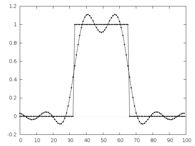
Fig. 3 Low-pass filtered version of a real pulse, output from the example program.
References and Further Reading
A good starting point for learning more about the FFT is the following review article,
P. Duhamel and M. Vetterli. Fast Fourier transforms: A tutorial review and a state of the art. Signal Processing, 19:259–299, 1990.
To find out about the algorithms used in the GSL routines you may want
to consult the document “GSL FFT Algorithms” (it is included
in GSL, as doc/fftalgorithms.tex). This has general information
on FFTs and explicit derivations of the implementation for each
routine. There are also references to the relevant literature. For
convenience some of the more important references are reproduced below.
There are several introductory books on the FFT with example programs, such as “The Fast Fourier Transform” by Brigham and “DFT/FFT and Convolution Algorithms” by Burrus and Parks,
Oran Brigham. “The Fast Fourier Transform”. Prentice Hall, 1974.
C. S. Burrus and T. W. Parks. “DFT/FFT and Convolution Algorithms”, Wiley, 1984.
Both these introductory books cover the radix-2 FFT in some detail. The mixed-radix algorithm at the heart of the FFTPACK routines is reviewed in Clive Temperton’s paper,
Clive Temperton, Self-sorting mixed-radix fast Fourier transforms, Journal of Computational Physics, 52(1):1–23, 1983.
The derivation of FFTs for real-valued data is explained in the following two articles,
Henrik V. Sorenson, Douglas L. Jones, Michael T. Heideman, and C. Sidney Burrus. Real-valued fast Fourier transform algorithms. “IEEE Transactions on Acoustics, Speech, and Signal Processing”, ASSP-35(6):849–863, 1987.
Clive Temperton. Fast mixed-radix real Fourier transforms. “Journal of Computational Physics”, 52:340–350, 1983.
In 1979 the IEEE published a compendium of carefully-reviewed Fortran FFT programs in “Programs for Digital Signal Processing”. It is a useful reference for implementations of many different FFT algorithms,
Digital Signal Processing Committee and IEEE Acoustics, Speech, and Signal Processing Committee, editors. Programs for Digital Signal Processing. IEEE Press, 1979.
For large-scale FFT work we recommend the use of the dedicated FFTW library by Frigo and Johnson. The FFTW library is self-optimizing—it automatically tunes itself for each hardware platform in order to achieve maximum performance. It is available under the GNU GPL.
FFTW Website, http://www.fftw.org/
The source code for FFTPACK is available from http://www.netlib.org/fftpack/