Multidimensional Minimization¶

This chapter describes routines for finding minima of arbitrary multidimensional functions. The library provides low level components for a variety of iterative minimizers and convergence tests. These can be combined by the user to achieve the desired solution, while providing full access to the intermediate steps of the algorithms. Each class of methods uses the same framework, so that you can switch between minimizers at runtime without needing to recompile your program. Each instance of a minimizer keeps track of its own state, allowing the minimizers to be used in multi-threaded programs. The minimization algorithms can be used to maximize a function by inverting its sign.

The header file gsl_multimin.h contains prototypes for the minimization functions and related declarations.

Overview¶

The problem of multidimensional minimization requires finding a point $x$ such that the scalar function,

$f(x_1, \dots, x_n)$

takes a value which is lower than at any neighboring point. For smooth functions the gradient $g = \nabla f$ vanishes at the minimum. In general there are no bracketing methods available for the minimization of $n$ -dimensional functions. The algorithms proceed from an initial guess using a search algorithm which attempts to move in a downhill direction.

Algorithms making use of the gradient of the function perform a one-dimensional line minimisation along this direction until the lowest point is found to a suitable tolerance. The search direction is then updated with local information from the function and its derivatives, and the whole process repeated until the true $n$ -dimensional minimum is found.

Algorithms which do not require the gradient of the function use different strategies. For example, the Nelder-Mead Simplex algorithm maintains $n+1$ trial parameter vectors as the vertices of a $n$ -dimensional simplex. On each iteration it tries to improve the worst vertex of the simplex by geometrical transformations. The iterations are continued until the overall size of the simplex has decreased sufficiently.

Both types of algorithms use a standard framework. The user provides a high-level driver for the algorithms, and the library provides the individual functions necessary for each of the steps. There are three main phases of the iteration. The steps are,

initialize minimizer state, s, for algorithm T
update s using the iteration T
test s for convergence, and repeat iteration if necessary

Each iteration step consists either of an improvement to the line-minimisation in the current direction or an update to the search direction itself. The state for the minimizers is held in a gsl_multimin_fdfminimizer struct or a gsl_multimin_fminimizer struct.

Caveats¶

Note that the minimization algorithms can only search for one local minimum at a time. When there are several local minima in the search area, the first minimum to be found will be returned; however it is difficult to predict which of the minima this will be. In most cases, no error will be reported if you try to find a local minimum in an area where there is more than one.

It is also important to note that the minimization algorithms find local minima; there is no way to determine whether a minimum is a global minimum of the function in question.

Initializing the Multidimensional Minimizer¶

The following function initializes a multidimensional minimizer. The minimizer itself depends only on the dimension of the problem and the algorithm and can be reused for different problems.

type gsl_multimin_fdfminimizer¶: This is a workspace for minimizing functions using derivatives.

type gsl_multimin_fminimizer¶: This is a workspace for minimizing functions without derivatives.

gsl_multimin_fdfminimizer *gsl_multimin_fdfminimizer_alloc(const gsl_multimin_fdfminimizer_type *T, size_t n)¶
gsl_multimin_fminimizer *gsl_multimin_fminimizer_alloc(const gsl_multimin_fminimizer_type *T, size_t n)¶: This function returns a pointer to a newly allocated instance of a minimizer of type T for an n-dimension function. If there is insufficient memory to create the minimizer then the function returns a null pointer and the error handler is invoked with an error code of GSL_ENOMEM.

int gsl_multimin_fdfminimizer_set(gsl_multimin_fdfminimizer *s, gsl_multimin_function_fdf *fdf, const gsl_vector *x, double step_size, double tol)¶

int gsl_multimin_fminimizer_set(gsl_multimin_fminimizer *s, gsl_multimin_function *f, const gsl_vector *x, const gsl_vector *step_size)¶

The function gsl_multimin_fdfminimizer_set() initializes the minimizer s to minimize the function fdf starting from the initial point x. The size of the first trial step is given by step_size. The accuracy of the line minimization is specified by tol. The precise meaning of this parameter depends on the method used. Typically the line minimization is considered successful if the gradient of the function $g$ is orthogonal to the current search direction $p$ to a relative accuracy of tol, where $p \cdot g < tol |p| |g|$ . A tol value of 0.1 is suitable for most purposes, since line minimization only needs to be carried out approximately. Note that setting tol to zero will force the use of “exact” line-searches, which are extremely expensive.

The function gsl_multimin_fminimizer_set() initializes the minimizer s to minimize the function f, starting from the initial point x. The size of the initial trial steps is given in vector step_size. The precise meaning of this parameter depends on the method used.

void gsl_multimin_fdfminimizer_free(gsl_multimin_fdfminimizer *s)¶
void gsl_multimin_fminimizer_free(gsl_multimin_fminimizer *s)¶: This function frees all the memory associated with the minimizer s.

const char *gsl_multimin_fdfminimizer_name(const gsl_multimin_fdfminimizer *s)¶

const char *gsl_multimin_fminimizer_name(const gsl_multimin_fminimizer *s)¶

This function returns a pointer to the name of the minimizer. For example:

printf ("s is a '%s' minimizer\n", gsl_multimin_fdfminimizer_name (s));

would print something like s is a 'conjugate_pr' minimizer.

Providing a function to minimize¶

You must provide a parametric function of $n$ variables for the minimizers to operate on. You may also need to provide a routine which calculates the gradient of the function and a third routine which calculates both the function value and the gradient together. In order to allow for general parameters the functions are defined by the following data types:

type gsl_multimin_function_fdf¶

This data type defines a general function of $n$ variables with parameters and the corresponding gradient vector of derivatives,

double (* f) (const gsl_vector * x, void * params)

this function should return the result $f(x,params)$ for argument x and parameters params. If the function cannot be computed, an error value of GSL_NAN should be returned.

void (* df) (const gsl_vector * x, void * params, gsl_vector * g)

this function should store the n-dimensional gradient

$g_i = \partial f(x,\hbox{\it params}) / \partial x_i$

in the vector g for argument x and parameters params, returning an appropriate error code if the function cannot be computed.

void (* fdf) (const gsl_vector * x, void * params, double * f, gsl_vector * g)

This function should set the values of the f and g as above, for arguments x and parameters params. This function provides an optimization of the separate functions for $f(x)$ and $g(x)$ —it is always faster to compute the function and its derivative at the same time.

size_t n

the dimension of the system, i.e. the number of components of the vectors x.

void * params

a pointer to the parameters of the function.

type gsl_multimin_function¶

This data type defines a general function of $n$ variables with parameters,

double (* f) (const gsl_vector * x, void * params)

this function should return the result $f(x,params)$ for argument x and parameters params. If the function cannot be computed, an error value of GSL_NAN should be returned.

size_t n

the dimension of the system, i.e. the number of components of the vectors x.

void * params

a pointer to the parameters of the function.

The following example function defines a simple two-dimensional paraboloid with five parameters,

/* Paraboloid centered on (p[0],p[1]), with
   scale factors (p[2],p[3]) and minimum p[4] */

double
my_f (const gsl_vector *v, void *params)
{
  double x, y;
  double *p = (double *)params;

  x = gsl_vector_get(v, 0);
  y = gsl_vector_get(v, 1);

  return p[2] * (x - p[0]) * (x - p[0]) +
           p[3] * (y - p[1]) * (y - p[1]) + p[4];
}

/* The gradient of f, df = (df/dx, df/dy). */
void
my_df (const gsl_vector *v, void *params,
       gsl_vector *df)
{
  double x, y;
  double *p = (double *)params;

  x = gsl_vector_get(v, 0);
  y = gsl_vector_get(v, 1);

  gsl_vector_set(df, 0, 2.0 * p[2] * (x - p[0]));
  gsl_vector_set(df, 1, 2.0 * p[3] * (y - p[1]));
}

/* Compute both f and df together. */
void
my_fdf (const gsl_vector *x, void *params,
        double *f, gsl_vector *df)
{
  *f = my_f(x, params);
  my_df(x, params, df);
}

The function can be initialized using the following code:

gsl_multimin_function_fdf my_func;

/* Paraboloid center at (1,2), scale factors (10, 20),
   minimum value 30 */
double p[5] = { 1.0, 2.0, 10.0, 20.0, 30.0 };

my_func.n = 2;  /* number of function components */
my_func.f = &my_f;
my_func.df = &my_df;
my_func.fdf = &my_fdf;
my_func.params = (void *)p;

Iteration¶

The following function drives the iteration of each algorithm. The function performs one iteration to update the state of the minimizer. The same function works for all minimizers so that different methods can be substituted at runtime without modifications to the code.

int gsl_multimin_fdfminimizer_iterate(gsl_multimin_fdfminimizer *s)¶
int gsl_multimin_fminimizer_iterate(gsl_multimin_fminimizer *s)¶: These functions perform a single iteration of the minimizer s. If the iteration encounters an unexpected problem then an error code will be returned. The error code GSL_ENOPROG signifies that the minimizer is unable to improve on its current estimate, either due to numerical difficulty or because a genuine local minimum has been reached.

The minimizer maintains a current best estimate of the minimum at all times. This information can be accessed with the following auxiliary functions,

gsl_vector *gsl_multimin_fdfminimizer_x(const gsl_multimin_fdfminimizer *s)¶
gsl_vector *gsl_multimin_fminimizer_x(const gsl_multimin_fminimizer *s)¶
double gsl_multimin_fdfminimizer_minimum(const gsl_multimin_fdfminimizer *s)¶
double gsl_multimin_fminimizer_minimum(const gsl_multimin_fminimizer *s)¶
gsl_vector *gsl_multimin_fdfminimizer_gradient(const gsl_multimin_fdfminimizer *s)¶
gsl_vector *gsl_multimin_fdfminimizer_dx(const gsl_multimin_fdfminimizer *s)¶
double gsl_multimin_fminimizer_size(const gsl_multimin_fminimizer *s)¶: These functions return the current best estimate of the location of the minimum, the value of the function at that point, its gradient, the last step increment of the estimate, and minimizer specific characteristic size for the minimizer s.

int gsl_multimin_fdfminimizer_restart(gsl_multimin_fdfminimizer *s)¶: This function resets the minimizer s to use the current point as a new starting point.

Stopping Criteria¶

A minimization procedure should stop when one of the following conditions is true:

A minimum has been found to within the user-specified precision.
A user-specified maximum number of iterations has been reached.
An error has occurred.

The handling of these conditions is under user control. The functions below allow the user to test the precision of the current result.

int gsl_multimin_test_gradient(const gsl_vector *g, double epsabs)¶

This function tests the norm of the gradient g against the absolute tolerance epsabs. The gradient of a multidimensional function goes to zero at a minimum. The test returns GSL_SUCCESS if the following condition is achieved,

$|g| < \hbox{\it epsabs}$

and returns GSL_CONTINUE otherwise. A suitable choice of epsabs can be made from the desired accuracy in the function for small variations in $x$ . The relationship between these quantities is given by $\delta{f} = g\,\delta{x}$ .

int gsl_multimin_test_size(const double size, double epsabs)¶: This function tests the minimizer specific characteristic size (if applicable to the used minimizer) against absolute tolerance epsabs. The test returns GSL_SUCCESS if the size is smaller than tolerance, otherwise GSL_CONTINUE is returned.

Algorithms with Derivatives¶

There are several minimization methods available. The best choice of algorithm depends on the problem. The algorithms described in this section use the value of the function and its gradient at each evaluation point.

type gsl_multimin_fdfminimizer_type¶

This type specifies a minimization algorithm using gradients.

gsl_multimin_fdfminimizer_type *gsl_multimin_fdfminimizer_conjugate_fr¶

This is the Fletcher-Reeves conjugate gradient algorithm. The conjugate gradient algorithm proceeds as a succession of line minimizations. The sequence of search directions is used to build up an approximation to the curvature of the function in the neighborhood of the minimum.

An initial search direction p is chosen using the gradient, and line minimization is carried out in that direction. The accuracy of the line minimization is specified by the parameter tol. The minimum along this line occurs when the function gradient g and the search direction p are orthogonal. The line minimization terminates when $p\cdot g < tol |p| |g|$ . The search direction is updated using the Fletcher-Reeves formula $p' = g' - \beta p$ where $\beta=-|g'|^2/|g|^2$ , and the line minimization is then repeated for the new search direction.

gsl_multimin_fdfminimizer_type *gsl_multimin_fdfminimizer_conjugate_pr¶: This is the Polak-Ribiere conjugate gradient algorithm. It is similar to the Fletcher-Reeves method, differing only in the choice of the coefficient $\beta$ . Both methods work well when the evaluation point is close enough to the minimum of the objective function that it is well approximated by a quadratic hypersurface.

gsl_multimin_fdfminimizer_type *gsl_multimin_fdfminimizer_vector_bfgs2¶

gsl_multimin_fdfminimizer_type *gsl_multimin_fdfminimizer_vector_bfgs¶

These methods use the vector Broyden-Fletcher-Goldfarb-Shanno (BFGS) algorithm. This is a quasi-Newton method which builds up an approximation to the second derivatives of the function $f$ using the difference between successive gradient vectors. By combining the first and second derivatives the algorithm is able to take Newton-type steps towards the function minimum, assuming quadratic behavior in that region.

The bfgs2 version of this minimizer is the most efficient version available, and is a faithful implementation of the line minimization scheme described in Fletcher’s Practical Methods of Optimization, Algorithms 2.6.2 and 2.6.4. It supersedes the original bfgs routine and requires substantially fewer function and gradient evaluations. The user-supplied tolerance tol corresponds to the parameter $\sigma$ used by Fletcher. A value of 0.1 is recommended for typical use (larger values correspond to less accurate line searches).

gsl_multimin_fdfminimizer_type *gsl_multimin_fdfminimizer_steepest_descent¶: The steepest descent algorithm follows the downhill gradient of the function at each step. When a downhill step is successful the step-size is increased by a factor of two. If the downhill step leads to a higher function value then the algorithm backtracks and the step size is decreased using the parameter tol. A suitable value of tol for most applications is 0.1. The steepest descent method is inefficient and is included only for demonstration purposes.

Algorithms without Derivatives¶

The algorithms described in this section use only the value of the function at each evaluation point.

type gsl_multimin_fminimizer_type¶

This type specifies minimization algorithms which do not use gradients.

gsl_multimin_fminimizer_type *gsl_multimin_fminimizer_nmsimplex2¶

gsl_multimin_fminimizer_type *gsl_multimin_fminimizer_nmsimplex¶

These methods use the Simplex algorithm of Nelder and Mead. Starting from the initial vector $x = p_0$ , the algorithm constructs an additional $n$ vectors $p_i$ using the step size vector $s = step\_size$ as follows:

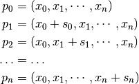
$p_0 & = (x_0, x_1, \cdots , x_n) \\ p_1 & = (x_0 + s_0, x_1, \cdots , x_n) \\ p_2 & = (x_0, x_1 + s_1, \cdots , x_n) \\ \dots &= \dots \\ p_n & = (x_0, x_1, \cdots , x_n + s_n)$

These vectors form the $n+1$ vertices of a simplex in $n$ dimensions. On each iteration the algorithm uses simple geometrical transformations to update the vector corresponding to the highest function value. The geometric transformations are reflection, reflection followed by expansion, contraction and multiple contraction. Using these transformations the simplex moves through the space towards the minimum, where it contracts itself.

After each iteration, the best vertex is returned. Note, that due to the nature of the algorithm not every step improves the current best parameter vector. Usually several iterations are required.

The minimizer-specific characteristic size is calculated as the average distance from the geometrical center of the simplex to all its vertices. This size can be used as a stopping criteria, as the simplex contracts itself near the minimum. The size is returned by the function gsl_multimin_fminimizer_size().

The gsl_multimin_fminimizer_nmsimplex2 version of this minimiser is a new $O(N)$ operations implementation of the earlier $O(N^2)$ operations gsl_multimin_fminimizer_nmsimplex minimiser. It uses the same underlying algorithm, but the simplex updates are computed more efficiently for high-dimensional problems. In addition, the size of simplex is calculated as the RMS distance of each vertex from the center rather than the mean distance, allowing a linear update of this quantity on each step. The memory usage is $O(N^2)$ for both algorithms.

gsl_multimin_fminimizer_type *gsl_multimin_fminimizer_nmsimplex2rand¶: This method is a variant of gsl_multimin_fminimizer_nmsimplex2 which initialises the simplex around the starting point x using a randomly-oriented set of basis vectors instead of the fixed coordinate axes. The final dimensions of the simplex are scaled along the coordinate axes by the vector step_size. The randomisation uses a simple deterministic generator so that repeated calls to gsl_multimin_fminimizer_set() for a given solver object will vary the orientation in a well-defined way.

Examples¶

This example program finds the minimum of the paraboloid function defined earlier. The location of the minimum is offset from the origin in $x$ and $y$ , and the function value at the minimum is non-zero. The main program is given below, it requires the example function given earlier in this chapter.

int
main (void)
{
  size_t iter = 0;
  int status;

  const gsl_multimin_fdfminimizer_type *T;
  gsl_multimin_fdfminimizer *s;

  /* Position of the minimum (1,2), scale factors
     10,20, height 30. */
  double par[5] = { 1.0, 2.0, 10.0, 20.0, 30.0 };

  gsl_vector *x;
  gsl_multimin_function_fdf my_func;

  my_func.n = 2;
  my_func.f = my_f;
  my_func.df = my_df;
  my_func.fdf = my_fdf;
  my_func.params = par;

  /* Starting point, x = (5,7) */
  x = gsl_vector_alloc (2);
  gsl_vector_set (x, 0, 5.0);
  gsl_vector_set (x, 1, 7.0);

  T = gsl_multimin_fdfminimizer_conjugate_fr;
  s = gsl_multimin_fdfminimizer_alloc (T, 2);

  gsl_multimin_fdfminimizer_set (s, &my_func, x, 0.01, 1e-4);

  do
    {
      iter++;
      status = gsl_multimin_fdfminimizer_iterate (s);

      if (status)
        break;

      status = gsl_multimin_test_gradient (s->gradient, 1e-3);

      if (status == GSL_SUCCESS)
        printf ("Minimum found at:\n");

      printf ("%5d %.5f %.5f %10.5f\n", iter,
              gsl_vector_get (s->x, 0),
              gsl_vector_get (s->x, 1),
              s->f);

    }
  while (status == GSL_CONTINUE && iter < 100);

  gsl_multimin_fdfminimizer_free (s);
  gsl_vector_free (x);

  return 0;
}

The initial step-size is chosen as 0.01, a conservative estimate in this case, and the line minimization parameter is set at 0.0001. The program terminates when the norm of the gradient has been reduced below 0.001. The output of the program is shown below,

         x       y         f
4.99629 6.99072  687.84780
4.98886 6.97215  683.55456
4.97400 6.93501  675.01278
4.94429 6.86073  658.10798
4.88487 6.71217  625.01340
4.76602 6.41506  561.68440
4.52833 5.82083  446.46694
4.05295 4.63238  261.79422
3.10219 2.25548   75.49762
2.85185 1.62963   67.03704
2.19088 1.76182   45.31640
0.86892 2.02622   30.18555
Minimum found at:
1.00000 2.00000   30.00000

Note that the algorithm gradually increases the step size as it successfully moves downhill, as can be seen by plotting the successive points in Fig. 29.

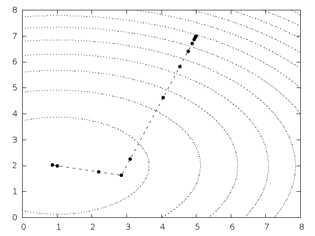
Fig. 29 Function contours with path taken by minimization algorithm¶

The conjugate gradient algorithm finds the minimum on its second direction because the function is purely quadratic. Additional iterations would be needed for a more complicated function.

Here is another example using the Nelder-Mead Simplex algorithm to minimize the same example object function, as above.

int
main(void)
{
  double par[5] = {1.0, 2.0, 10.0, 20.0, 30.0};

  const gsl_multimin_fminimizer_type *T =
    gsl_multimin_fminimizer_nmsimplex2;
  gsl_multimin_fminimizer *s = NULL;
  gsl_vector *ss, *x;
  gsl_multimin_function minex_func;

  size_t iter = 0;
  int status;
  double size;

  /* Starting point */
  x = gsl_vector_alloc (2);
  gsl_vector_set (x, 0, 5.0);
  gsl_vector_set (x, 1, 7.0);

  /* Set initial step sizes to 1 */
  ss = gsl_vector_alloc (2);
  gsl_vector_set_all (ss, 1.0);

  /* Initialize method and iterate */
  minex_func.n = 2;
  minex_func.f = my_f;
  minex_func.params = par;

  s = gsl_multimin_fminimizer_alloc (T, 2);
  gsl_multimin_fminimizer_set (s, &minex_func, x, ss);

  do
    {
      iter++;
      status = gsl_multimin_fminimizer_iterate(s);

      if (status)
        break;

      size = gsl_multimin_fminimizer_size (s);
      status = gsl_multimin_test_size (size, 1e-2);

      if (status == GSL_SUCCESS)
        {
          printf ("converged to minimum at\n");
        }

      printf ("%5d %10.3e %10.3e f() = %7.3f size = %.3f\n",
              iter,
              gsl_vector_get (s->x, 0),
              gsl_vector_get (s->x, 1),
              s->fval, size);
    }
  while (status == GSL_CONTINUE && iter < 100);

  gsl_vector_free(x);
  gsl_vector_free(ss);
  gsl_multimin_fminimizer_free (s);

  return status;
}

The minimum search stops when the Simplex size drops to 0.01. The output is shown below.

6.500e+00  5.000e+00 f() = 512.500 size = 1.130
5.250e+00  4.000e+00 f() = 290.625 size = 1.409
5.250e+00  4.000e+00 f() = 290.625 size = 1.409
5.500e+00  1.000e+00 f() = 252.500 size = 1.409
2.625e+00  3.500e+00 f() = 101.406 size = 1.847
2.625e+00  3.500e+00 f() = 101.406 size = 1.847
0.000e+00  3.000e+00 f() =  60.000 size = 1.847
2.094e+00  1.875e+00 f() =  42.275 size = 1.321
2.578e-01  1.906e+00 f() =  35.684 size = 1.069
5.879e-01  2.445e+00 f() =  35.664 size = 0.841
1.258e+00  2.025e+00 f() =  30.680 size = 0.476
1.258e+00  2.025e+00 f() =  30.680 size = 0.367
1.093e+00  1.849e+00 f() =  30.539 size = 0.300
8.830e-01  2.004e+00 f() =  30.137 size = 0.172
8.830e-01  2.004e+00 f() =  30.137 size = 0.126
9.582e-01  2.060e+00 f() =  30.090 size = 0.106
1.022e+00  2.004e+00 f() =  30.005 size = 0.063
1.022e+00  2.004e+00 f() =  30.005 size = 0.043
1.022e+00  2.004e+00 f() =  30.005 size = 0.043
1.022e+00  2.004e+00 f() =  30.005 size = 0.027
1.022e+00  2.004e+00 f() =  30.005 size = 0.022
9.920e-01  1.997e+00 f() =  30.001 size = 0.016
9.920e-01  1.997e+00 f() =  30.001 size = 0.013
converged to minimum at
9.920e-01  1.997e+00 f() =  30.001 size = 0.008

The simplex size first increases, while the simplex moves towards the minimum. After a while the size begins to decrease as the simplex contracts around the minimum.

References and Further Reading¶

The conjugate gradient and BFGS methods are described in detail in the following book,

R. Fletcher, Practical Methods of Optimization (Second Edition) Wiley (1987), ISBN 0471915475.

A brief description of multidimensional minimization algorithms and more recent references can be found in,

C.W. Ueberhuber, Numerical Computation (Volume 2), Chapter 14, Section 4.4 “Minimization Methods”, p.: 325–335, Springer (1997), ISBN 3-540-62057-5.

The simplex algorithm is described in the following paper,

J.A. Nelder and R. Mead, A simplex method for function minimization, Computer Journal vol.: 7 (1965), 308–313.