Numerical Integration
This chapter describes routines for performing numerical integration (quadrature) of a function in one dimension. There are routines for adaptive and non-adaptive integration of general functions, with specialised routines for specific cases. These include integration over infinite and semi-infinite ranges, singular integrals, including logarithmic singularities, computation of Cauchy principal values and oscillatory integrals. The library reimplements the algorithms used in QUADPACK, a numerical integration package written by Piessens, de Doncker-Kapenga, Ueberhuber and Kahaner. Fortran code for QUADPACK is available on Netlib. Also included are non-adaptive, fixed-order Gauss-Legendre integration routines with high precision coefficients, as well as fixed-order quadrature rules for a variety of weighting functions from IQPACK.
The functions described in this chapter are declared in the header file
gsl_integration.h.
Introduction
Each algorithm computes an approximation to a definite integral of the form,
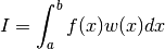
where  is a weight function (for general integrands
  ).
The user provides absolute and relative error bounds
).
The user provides absolute and relative error bounds
 which specify the following accuracy requirement,

where  is the numerical approximation obtained by the
algorithm. The algorithms attempt to estimate the absolute error
is the numerical approximation obtained by the
algorithm. The algorithms attempt to estimate the absolute error
 in such a way that the following inequality
holds,
in such a way that the following inequality
holds,

In short, the routines return the first approximation
which has an absolute error smaller than
 or a relative error smaller than
  .
.
Note that this is an either-or constraint,
not simultaneous. To compute to a specified absolute error, set
to zero. To compute to a specified relative error,
set to zero.
The routines will fail to converge if the error bounds are too
stringent, but always return the best approximation obtained up to
that stage.
The algorithms in QUADPACK use a naming convention based on the following letters:
Q - quadrature routine

N - non-adaptive integrator
A - adaptive integrator

G - general integrand (user-defined)
W - weight function with integrand

S - singularities can be more readily integrated
P - points of special difficulty can be supplied
I - infinite range of integration
O - oscillatory weight function, cos or sin
F - Fourier integral
C - Cauchy principal value
The algorithms are built on pairs of quadrature rules, a higher order rule and a lower order rule. The higher order rule is used to compute the best approximation to an integral over a small range. The difference between the results of the higher order rule and the lower order rule gives an estimate of the error in the approximation.
Integrands without weight functions
The algorithms for general functions (without a weight function) are based on Gauss-Kronrod rules.
A Gauss-Kronrod rule begins with a classical Gaussian quadrature rule of
order  . This is extended with additional points between each of
the abscissae to give a higher order Kronrod rule of order
. This is extended with additional points between each of
the abscissae to give a higher order Kronrod rule of order  .
The Kronrod rule is efficient because it reuses existing function
evaluations from the Gaussian rule.
.
The Kronrod rule is efficient because it reuses existing function
evaluations from the Gaussian rule.
The higher order Kronrod rule is used as the best approximation to the integral, and the difference between the two rules is used as an estimate of the error in the approximation.
Integrands with weight functions
For integrands with weight functions the algorithms use Clenshaw-Curtis quadrature rules.
A Clenshaw-Curtis rule begins with an  -th order Chebyshev
polynomial approximation to the integrand. This polynomial can be
integrated exactly to give an approximation to the integral of the
original function. The Chebyshev expansion can be extended to higher
orders to improve the approximation and provide an estimate of the
error.
-th order Chebyshev
polynomial approximation to the integrand. This polynomial can be
integrated exactly to give an approximation to the integral of the
original function. The Chebyshev expansion can be extended to higher
orders to improve the approximation and provide an estimate of the
error.
Integrands with singular weight functions
The presence of singularities (or other behavior) in the integrand can cause slow convergence in the Chebyshev approximation. The modified Clenshaw-Curtis rules used in QUADPACK separate out several common weight functions which cause slow convergence.
These weight functions are integrated analytically against the Chebyshev polynomials to precompute modified Chebyshev moments. Combining the moments with the Chebyshev approximation to the function gives the desired integral. The use of analytic integration for the singular part of the function allows exact cancellations and substantially improves the overall convergence behavior of the integration.
QNG non-adaptive Gauss-Kronrod integration
The QNG algorithm is a non-adaptive procedure which uses fixed Gauss-Kronrod-Patterson abscissae to sample the integrand at a maximum of 87 points. It is provided for fast integration of smooth functions.
-
int gsl_integration_qng(const gsl_function *f, double a, double b, double epsabs, double epsrel, double *result, double *abserr, size_t *neval)
This function applies the Gauss-Kronrod 10-point, 21-point, 43-point and 87-point integration rules in succession until an estimate of the integral of
 over
over  is achieved within the desired
absolute and relative error limits,
is achieved within the desired
absolute and relative error limits, epsabsandepsrel. The function returns the final approximation,result, an estimate of the absolute error,abserrand the number of function evaluations used,neval. The Gauss-Kronrod rules are designed in such a way that each rule uses all the results of its predecessors, in order to minimize the total number of function evaluations.
QAG adaptive integration
The QAG algorithm is a simple adaptive integration procedure. The integration region is divided into subintervals, and on each iteration the subinterval with the largest estimated error is bisected. This reduces the overall error rapidly, as the subintervals become concentrated around local difficulties in the integrand. These subintervals are managed by the following struct,
-
type gsl_integration_workspace
This workspace handles the memory for the subinterval ranges, results and error estimates.
-
gsl_integration_workspace *gsl_integration_workspace_alloc(size_t n)
This function allocates a workspace sufficient to hold
ndouble precision intervals, their integration results and error estimates. One workspace may be used multiple times as all necessary reinitialization is performed automatically by the integration routines.
-
void gsl_integration_workspace_free(gsl_integration_workspace *w)
This function frees the memory associated with the workspace
w.
-
int gsl_integration_qag(const gsl_function *f, double a, double b, double epsabs, double epsrel, size_t limit, int key, gsl_integration_workspace *workspace, double *result, double *abserr)
This function applies an integration rule adaptively until an estimate of the integral of
over is achieved within the
desired absolute and relative error limits, epsabsandepsrel. The function returns the final approximation,result, and an estimate of the absolute error,abserr. The integration rule is determined by the value ofkey, which should be chosen from the following symbolic names,Symbolic Name
Key
GSL_INTEG_GAUSS151
GSL_INTEG_GAUSS212
GSL_INTEG_GAUSS313
GSL_INTEG_GAUSS414
GSL_INTEG_GAUSS515
GSL_INTEG_GAUSS616
corresponding to the 15, 21, 31, 41, 51 and 61 point Gauss-Kronrod rules. The higher-order rules give better accuracy for smooth functions, while lower-order rules save time when the function contains local difficulties, such as discontinuities.
On each iteration the adaptive integration strategy bisects the interval with the largest error estimate. The subintervals and their results are stored in the memory provided by
workspace. The maximum number of subintervals is given bylimit, which may not exceed the allocated size of the workspace.
QAGS adaptive integration with singularities
The presence of an integrable singularity in the integration region causes an adaptive routine to concentrate new subintervals around the singularity. As the subintervals decrease in size the successive approximations to the integral converge in a limiting fashion. This approach to the limit can be accelerated using an extrapolation procedure. The QAGS algorithm combines adaptive bisection with the Wynn epsilon-algorithm to speed up the integration of many types of integrable singularities.
-
int gsl_integration_qags(const gsl_function *f, double a, double b, double epsabs, double epsrel, size_t limit, gsl_integration_workspace *workspace, double *result, double *abserr)
This function applies the Gauss-Kronrod 21-point integration rule adaptively until an estimate of the integral of
over
is achieved within the desired absolute and relative error
limits, epsabsandepsrel. The results are extrapolated using the epsilon-algorithm, which accelerates the convergence of the integral in the presence of discontinuities and integrable singularities. The function returns the final approximation from the extrapolation,result, and an estimate of the absolute error,abserr. The subintervals and their results are stored in the memory provided byworkspace. The maximum number of subintervals is given bylimit, which may not exceed the allocated size of the workspace.
QAGP adaptive integration with known singular points
-
int gsl_integration_qagp(const gsl_function *f, double *pts, size_t npts, double epsabs, double epsrel, size_t limit, gsl_integration_workspace *workspace, double *result, double *abserr)
This function applies the adaptive integration algorithm QAGS taking account of the user-supplied locations of singular points. The array
ptsof lengthnptsshould contain the endpoints of the integration ranges defined by the integration region and locations of the singularities. For example, to integrate over the region with break-points at  (where
 ) the following
 ptsarray should be used:pts[0] = a pts[1] = x_1 pts[2] = x_2 pts[3] = x_3 pts[4] = b
with
npts= 5.If you know the locations of the singular points in the integration region then this routine will be faster than
gsl_integration_qags().
QAGI adaptive integration on infinite intervals
-
int gsl_integration_qagi(gsl_function *f, double epsabs, double epsrel, size_t limit, gsl_integration_workspace *workspace, double *result, double *abserr)
This function computes the integral of the function
fover the infinite interval . The integral is mapped onto the
semi-open interval
. The integral is mapped onto the
semi-open interval ![(0,1]](_images/math/a0063095d691b496eed43bd797d9f2a70fb01541.png) using the transformation
using the transformation  ,
,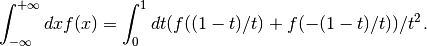
It is then integrated using the QAGS algorithm. The normal 21-point Gauss-Kronrod rule of QAGS is replaced by a 15-point rule, because the transformation can generate an integrable singularity at the origin. In this case a lower-order rule is more efficient.
-
int gsl_integration_qagiu(gsl_function *f, double a, double epsabs, double epsrel, size_t limit, gsl_integration_workspace *workspace, double *result, double *abserr)
This function computes the integral of the function
fover the semi-infinite interval . The integral is mapped onto the
semi-open interval using the transformation
. The integral is mapped onto the
semi-open interval using the transformation 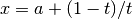 ,
,
and then integrated using the QAGS algorithm.
-
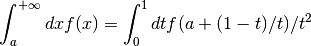
int gsl_integration_qagil(gsl_function *f, double b, double epsabs, double epsrel, size_t limit, gsl_integration_workspace *workspace, double *result, double *abserr)
This function computes the integral of the function
fover the semi-infinite interval . The integral is mapped onto the
semi-open interval using the transformation
. The integral is mapped onto the
semi-open interval using the transformation 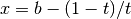 ,
,
and then integrated using the QAGS algorithm.
QAWC adaptive integration for Cauchy principal values
-
int gsl_integration_qawc(gsl_function *f, double a, double b, double c, double epsabs, double epsrel, size_t limit, gsl_integration_workspace *workspace, double *result, double *abserr)
This function computes the Cauchy principal value of the integral of
over , with a singularity at c,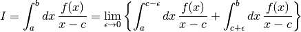
The adaptive bisection algorithm of QAG is used, with modifications to ensure that subdivisions do not occur at the singular point
 .
When a subinterval contains the point or is close to
it then a special 25-point modified Clenshaw-Curtis rule is used to control
the singularity. Further away from the
singularity the algorithm uses an ordinary 15-point Gauss-Kronrod
integration rule.
.
When a subinterval contains the point or is close to
it then a special 25-point modified Clenshaw-Curtis rule is used to control
the singularity. Further away from the
singularity the algorithm uses an ordinary 15-point Gauss-Kronrod
integration rule.
QAWS adaptive integration for singular functions
The QAWS algorithm is designed for integrands with algebraic-logarithmic singularities at the end-points of an integration region. In order to work efficiently the algorithm requires a precomputed table of Chebyshev moments.
-
type gsl_integration_qaws_table
This structure contains precomputed quantities for the QAWS algorithm.
-
gsl_integration_qaws_table *gsl_integration_qaws_table_alloc(double alpha, double beta, int mu, int nu)
This function allocates space for a
gsl_integration_qaws_tablestruct describing a singular weight function with the parameters  ,
,
where
 ,
,  , and
, and  ,
,
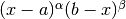
 . The weight function can take four different forms
depending on the values of
. The weight function can take four different forms
depending on the values of  and
and  ,
,Weight function


The singular points
do not have to be specified until the
integral is computed, where they are the endpoints of the integration
range.The function returns a pointer to the newly allocated table
gsl_integration_qaws_tableif no errors were detected, and 0 in the case of error.
-
int gsl_integration_qaws_table_set(gsl_integration_qaws_table *t, double alpha, double beta, int mu, int nu)
This function modifies the parameters
of
an existing gsl_integration_qaws_tablestructt.
-
void gsl_integration_qaws_table_free(gsl_integration_qaws_table *t)
This function frees all the memory associated with the
gsl_integration_qaws_tablestructt.
-
int gsl_integration_qaws(gsl_function *f, const double a, const double b, gsl_integration_qaws_table *t, const double epsabs, const double epsrel, const size_t limit, gsl_integration_workspace *workspace, double *result, double *abserr)
This function computes the integral of the function
 over the
interval with the singular weight function
over the
interval with the singular weight function
 . The parameters
of the weight function are taken from the
table
. The parameters
of the weight function are taken from the
table t. The integral is,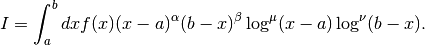
The adaptive bisection algorithm of QAG is used. When a subinterval contains one of the endpoints then a special 25-point modified Clenshaw-Curtis rule is used to control the singularities. For subintervals which do not include the endpoints an ordinary 15-point Gauss-Kronrod integration rule is used.
QAWO adaptive integration for oscillatory functions
The QAWO algorithm is designed for integrands with an oscillatory
factor,  or
or  . In order to
work efficiently the algorithm requires a table of Chebyshev moments
which must be pre-computed with calls to the functions below.
. In order to
work efficiently the algorithm requires a table of Chebyshev moments
which must be pre-computed with calls to the functions below.
-
gsl_integration_qawo_table *gsl_integration_qawo_table_alloc(double omega, double L, enum gsl_integration_qawo_enum sine, size_t n)
This function allocates space for a
gsl_integration_qawo_tablestruct and its associated workspace describing a sine or cosine weight function with the parameters  ,
,
The parameter
Lmust be the length of the interval over which the function will be integrated . The choice of sine or
cosine is made with the parameter
. The choice of sine or
cosine is made with the parameter sinewhich should be chosen from one of the two following symbolic values:-
GSL_INTEG_COSINE
-
GSL_INTEG_SINE
The
gsl_integration_qawo_tableis a table of the trigonometric coefficients required in the integration process. The parameterndetermines the number of levels of coefficients that are computed. Each level corresponds to one bisection of the interval , so that
nlevels are sufficient for subintervals down to the length . The integration routine
 gsl_integration_qawo()returns the errorGSL_ETABLEif the number of levels is insufficient for the requested accuracy.-
GSL_INTEG_COSINE
-
int gsl_integration_qawo_table_set(gsl_integration_qawo_table *t, double omega, double L, enum gsl_integration_qawo_enum sine)
This function changes the parameters
omega,Landsineof the existing workspacet.
-
int gsl_integration_qawo_table_set_length(gsl_integration_qawo_table *t, double L)
This function allows the length parameter
Lof the workspacetto be changed.
-
void gsl_integration_qawo_table_free(gsl_integration_qawo_table *t)
This function frees all the memory associated with the workspace
t.
-
int gsl_integration_qawo(gsl_function *f, const double a, const double epsabs, const double epsrel, const size_t limit, gsl_integration_workspace *workspace, gsl_integration_qawo_table *wf, double *result, double *abserr)
This function uses an adaptive algorithm to compute the integral of
over with the weight function
or defined
by the table wf,
The results are extrapolated using the epsilon-algorithm to accelerate the convergence of the integral. The function returns the final approximation from the extrapolation,
result, and an estimate of the absolute error,abserr. The subintervals and their results are stored in the memory provided byworkspace. The maximum number of subintervals is given bylimit, which may not exceed the allocated size of the workspace.Those subintervals with “large” widths
 where
where  are
computed using a 25-point Clenshaw-Curtis integration rule, which handles the
oscillatory behavior. Subintervals with a “small” widths where
are
computed using a 25-point Clenshaw-Curtis integration rule, which handles the
oscillatory behavior. Subintervals with a “small” widths where
 are computed using a 15-point Gauss-Kronrod integration.
QAWF adaptive integration for Fourier integrals
-
int gsl_integration_qawf(gsl_function *f, const double a, const double epsabs, const size_t limit, gsl_integration_workspace *workspace, gsl_integration_workspace *cycle_workspace, gsl_integration_qawo_table *wf, double *result, double *abserr)
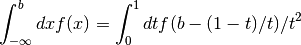
This function attempts to compute a Fourier integral of the function
fover the semi-infinite interval
The parameter
 and choice of
  or
or  is
taken from the table
is
taken from the table wf(the lengthLcan take any value, since it is overridden by this function to a value appropriate for the Fourier integration). The integral is computed using the QAWO algorithm over each of the subintervals,![C_1 &= [a,a+c] \\
C_2 &= [a+c,a+2c] \\
\dots &= \dots \\
C_k &= [a+(k-1)c,a+kc]](_images/math/4b4ba4d61ec98feec47edfcc9e1ddd2ac6f26f65.png)
where
 . The width
  is
chosen to cover an odd number of periods so that the contributions from
the intervals alternate in sign and are monotonically decreasing when
is
chosen to cover an odd number of periods so that the contributions from
the intervals alternate in sign and are monotonically decreasing when
fis positive and monotonically decreasing. The sum of this sequence of contributions is accelerated using the epsilon-algorithm.This function works to an overall absolute tolerance of
abserr. The following strategy is used: on each interval the algorithm tries to achieve the tolerance
where
 and
and  .
The sum of the geometric series of contributions from each interval
gives an overall tolerance of
.
The sum of the geometric series of contributions from each interval
gives an overall tolerance of abserr.If the integration of a subinterval leads to difficulties then the accuracy requirement for subsequent intervals is relaxed,
where
 is the estimated error on the interval .
The subintervals and their results are stored in the memory provided by
workspace. The maximum number of subintervals is given bylimit, which may not exceed the allocated size of the workspace. The integration over each subinterval uses the memory provided bycycle_workspaceas workspace for the QAWO algorithm.
CQUAD doubly-adaptive integration
CQUAD is a new doubly-adaptive general-purpose quadrature
routine which can handle most types of singularities,
non-numerical function values such as Inf or NaN,
as well as some divergent integrals. It generally requires more
function evaluations than the integration routines in
QUADPACK, yet fails less often for difficult integrands.
The underlying algorithm uses a doubly-adaptive scheme in which
Clenshaw-Curtis quadrature rules of increasing degree are used
to compute the integral in each interval. The  -norm of
the difference between the underlying interpolatory polynomials
of two successive rules is used as an error estimate. The
interval is subdivided if the difference between two successive
rules is too large or a rule of maximum degree has been reached.
-norm of
the difference between the underlying interpolatory polynomials
of two successive rules is used as an error estimate. The
interval is subdivided if the difference between two successive
rules is too large or a rule of maximum degree has been reached.
-
gsl_integration_cquad_workspace *gsl_integration_cquad_workspace_alloc(size_t n)
This function allocates a workspace sufficient to hold the data for
nintervals. The numbernis not the maximum number of intervals that will be evaluated. If the workspace is full, intervals with smaller error estimates will be discarded. A minimum of 3 intervals is required and for most functions, a workspace of size 100 is sufficient.
-
void gsl_integration_cquad_workspace_free(gsl_integration_cquad_workspace *w)
This function frees the memory associated with the workspace
w.
-
int gsl_integration_cquad(const gsl_function *f, double a, double b, double epsabs, double epsrel, gsl_integration_cquad_workspace *workspace, double *result, double *abserr, size_t *nevals)
This function computes the integral of
over
within the desired absolute and relative error limits, epsabsandepsrelusing the CQUAD algorithm. The function returns the final approximation,result, an estimate of the absolute error,abserr, and the number of function evaluations required,nevals.The CQUAD algorithm divides the integration region into subintervals, and in each iteration, the subinterval with the largest estimated error is processed. The algorithm uses Clenshaw-Curtis quadrature rules of degree 4, 8, 16 and 32 over 5, 9, 17 and 33 nodes respectively. Each interval is initialized with the lowest-degree rule. When an interval is processed, the next-higher degree rule is evaluated and an error estimate is computed based on the
-norm of the difference between the underlying interpolating
polynomials of both rules. If the highest-degree rule has already been
used, or the interpolatory polynomials differ significantly, the
interval is bisected.The subintervals and their results are stored in the memory provided by
workspace. If the error estimate or the number of function evaluations is not needed, the pointersabserrandnevalscan be set toNULL.
Romberg integration
The Romberg integration method estimates the definite integral
by applying Richardson extrapolation on the trapezoidal rule, using equally spaced points with spacing
for  . For each
  , Richardson extrapolation
is used
, Richardson extrapolation
is used  times on previous approximations to improve the order
of accuracy as much as possible. Romberg integration typically works
well (and converges quickly) for smooth integrands with no singularities in
the interval or at the end points.
times on previous approximations to improve the order
of accuracy as much as possible. Romberg integration typically works
well (and converges quickly) for smooth integrands with no singularities in
the interval or at the end points.
-
gsl_integration_romberg_workspace *gsl_integration_romberg_alloc(const size_t n)
This function allocates a workspace for Romberg integration, specifying a maximum of
iterations, or divisions of the interval. Since
the number of divisions is  , can be kept relatively
small (i.e.
, can be kept relatively
small (i.e.  or
or  ). It is capped at a maximum value of
 to prevent overflow. The size of the workspace is
  .
.
-
void gsl_integration_romberg_free(gsl_integration_romberg_workspace *w)
This function frees the memory associated with the workspace
w.
-
int gsl_integration_romberg(const gsl_function *f, const double a, const double b, const double epsabs, const double epsrel, double *result, size_t *neval, gsl_integration_romberg_workspace *w)
This function integrates
, specified by f, fromatob, storing the answer inresult. At each step in the iteration, convergence is tested by checking:
where
 is the current approximation and
  is the approximation
of the previous iteration. If the method does not converge within the previously
specified iterations, the function stores the best current estimate in
is the approximation
of the previous iteration. If the method does not converge within the previously
specified iterations, the function stores the best current estimate in
resultand returnsGSL_EMAXITER. If the method converges, the function returnsGSL_SUCCESS. The total number of function evaluations is returned inneval.
Gauss-Legendre integration
The fixed-order Gauss-Legendre integration routines are provided for fast
integration of smooth functions with known polynomial order. The
-point Gauss-Legendre rule is exact for polynomials of order
 or less. For example, these rules are useful when integrating
basis functions to form mass matrices for the Galerkin method. Unlike other
numerical integration routines within the library, these routines do not accept
absolute or relative error bounds.
or less. For example, these rules are useful when integrating
basis functions to form mass matrices for the Galerkin method. Unlike other
numerical integration routines within the library, these routines do not accept
absolute or relative error bounds.
-
gsl_integration_glfixed_table *gsl_integration_glfixed_table_alloc(size_t n)
This function determines the Gauss-Legendre abscissae and weights necessary for an
-point fixed order integration scheme. If possible, high precision
precomputed coefficients are used. If precomputed weights are not available,
lower precision coefficients are computed on the fly.
-
double gsl_integration_glfixed(const gsl_function *f, double a, double b, const gsl_integration_glfixed_table *t)
This function applies the Gauss-Legendre integration rule contained in table
tand returns the result.
-
int gsl_integration_glfixed_point(double a, double b, size_t i, double *xi, double *wi, const gsl_integration_glfixed_table *t)
For
iin![[0, \dots, n - 1]](_images/math/aa265b7178a163409df4e3c362d2368c688fe40d.png) , this function obtains the
, this function obtains the
i-th Gauss-Legendre pointxiand weightwion the interval [a,b]. The points and weights are ordered by increasing point value. A function may be integrated on [a,b] by summing over
over i.
Fixed point quadratures
The routines in this section approximate an integral by the sum
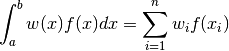
where is the function to be integrated and is
a weighting function. The weights  and nodes
  are carefully chosen
so that the result is exact when is a polynomial of degree
or less. Once the user chooses the order and weighting function , the
weights and nodes can be precomputed and used to efficiently evaluate
integrals for any number of functions .
are carefully chosen
so that the result is exact when is a polynomial of degree
or less. Once the user chooses the order and weighting function , the
weights and nodes can be precomputed and used to efficiently evaluate
integrals for any number of functions .
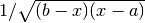
This method works best when is well approximated by a polynomial on the interval
, and so is not suitable for functions with singularities.
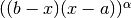
Since the user specifies ahead of time how many quadrature nodes will be used, these
routines do not accept absolute or relative error bounds. The table below lists
the weighting functions currently supported.
Name |
Interval |
Weighting function |
Constraints |
|---|---|---|---|
Legendre |
|
|
|
Chebyshev Type 1 |
|
|
|
Gegenbauer |
|
|
|
Jacobi |
|
|
|
Laguerre |
|
|
|
Hermite |
|
|
|
Exponential |
|
|
|
Rational |
|
|
|
Chebyshev Type 2 |
|
|
|


The fixed point quadrature routines use the following workspace to store the nodes and weights, as well as additional variables for intermediate calculations:
-
type gsl_integration_fixed_workspace
This workspace is used for fixed point quadrature rules and looks like this:
typedef struct
{
  size_t n;        /* number of nodes/weights */
  double *weights; /* quadrature weights */
  double *x;       /* quadrature nodes */
  double *diag;    /* diagonal of Jacobi matrix */
  double *subdiag; /* subdiagonal of Jacobi matrix */
  const gsl_integration_fixed_type * type;
} gsl_integration_fixed_workspace;
-
gsl_integration_fixed_workspace *gsl_integration_fixed_alloc(const gsl_integration_fixed_type *T, const size_t n, const double a, const double b, const double alpha, const double beta)
This function allocates a workspace for computing integrals with interpolating quadratures using
nquadrature nodes. The parametersa,b,alpha, andbetaspecify the integration interval and/or weighting function for the various quadrature types. See the table above for constraints on these parameters. The size of the workspace is .
.-
type gsl_integration_fixed_type
The type of quadrature used is specified by
Twhich can be set to the following choices:-
gsl_integration_fixed_type *gsl_integration_fixed_legendre
This specifies Legendre quadrature integration. The parameters
alphaandbetaare ignored for this type.
-
gsl_integration_fixed_type *gsl_integration_fixed_chebyshev
This specifies Chebyshev type 1 quadrature integration. The parameters
alphaandbetaare ignored for this type.
-
gsl_integration_fixed_type *gsl_integration_fixed_gegenbauer
This specifies Gegenbauer quadrature integration. The parameter
betais ignored for this type.
-
gsl_integration_fixed_type *gsl_integration_fixed_jacobi
This specifies Jacobi quadrature integration.
-
gsl_integration_fixed_type *gsl_integration_fixed_laguerre
This specifies Laguerre quadrature integration. The parameter
betais ignored for this type.
-
gsl_integration_fixed_type *gsl_integration_fixed_hermite
This specifies Hermite quadrature integration. The parameter
betais ignored for this type.
-
gsl_integration_fixed_type *gsl_integration_fixed_exponential
This specifies exponential quadrature integration. The parameter
betais ignored for this type.
-
gsl_integration_fixed_type *gsl_integration_fixed_rational
This specifies rational quadrature integration.
-
gsl_integration_fixed_type *gsl_integration_fixed_chebyshev2
This specifies Chebyshev type 2 quadrature integration. The parameters
alphaandbetaare ignored for this type.
-
gsl_integration_fixed_type *gsl_integration_fixed_legendre
-
type gsl_integration_fixed_type
-
void gsl_integration_fixed_free(gsl_integration_fixed_workspace *w)
This function frees the memory assocated with the workspace
w
-
size_t gsl_integration_fixed_n(const gsl_integration_fixed_workspace *w)
This function returns the number of quadrature nodes and weights.
-
double *gsl_integration_fixed_nodes(const gsl_integration_fixed_workspace *w)
This function returns a pointer to an array of size
ncontaining the quadrature nodes.
-
double *gsl_integration_fixed_weights(const gsl_integration_fixed_workspace *w)
This function returns a pointer to an array of size
ncontaining the quadrature weights.
-
int gsl_integration_fixed(const gsl_function *func, double *result, const gsl_integration_fixed_workspace *w)
This function integrates the function
provided in funcusing previously computed fixed quadrature rules. The integral is approximated as
where
are the quadrature weights and are the quadrature nodes computed
previously by gsl_integration_fixed_alloc(). The sum is stored inresulton output.
Integrating on the unit sphere
This section contains routines to calculate the surface integral of a function over the unit sphere,
![I[f] = \int d\Omega f(\Omega) = \int_0^{\pi} \sin{\theta} d\theta \int_0^{2\pi} d\phi f(\theta,\phi)](_images/math/3ed06d12c506ad475a3464d67035b4f340d7cfc3.png)
Lebedev developed a quadrature scheme to approximate this integral using a single sum,
![I[f] \approx 4 \pi \sum_{i=1}^n w_i f(\theta_i, \phi_i)](_images/math/39d288c70fd7bfacf8042e9edacdc02574f657ec.png)
for appropriately chosen weights and nodes  .
The Lebedev nodes are chosen to lie on the unit sphere and be invariant
under the octahedral rotation group with inversion.
.
The Lebedev nodes are chosen to lie on the unit sphere and be invariant
under the octahedral rotation group with inversion.
The number of quadrature nodes is often chosen in order to exactly
integrate a certain degree spherical harmonic function  .
A general rule of thumb for integrating spherical harmonics up to degree
and order is to choose the number of nodes as,
.
A general rule of thumb for integrating spherical harmonics up to degree
and order is to choose the number of nodes as,

Calculating the Lebedev weights and nodes requires solving a set of nonlinear equations. These equations have been solved, and the nodes and weights have been tabulated for integrating spherical harmonics up to degree and order 131. GSL offers a smaller subset of 32 quadrature rules, which are listed in the table below.
Spherical Harmonic degree |
Quadrature weights and nodes |
|---|---|
3 |
6 |
5 |
14 |
7 |
26 |
9 |
38 |
11 |
50 |
13 |
74 |
15 |
86 |
17 |
110 |
19 |
146 |
21 |
170 |
23 |
194 |
25 |
230 |
27 |
266 |
29 |
302 |
31 |
350 |
35 |
434 |
41 |
590 |
47 |
770 |
53 |
974 |
59 |
1202 |
65 |
1454 |
71 |
1730 |
77 |
2030 |
83 |
2354 |
89 |
2702 |
95 |
3074 |
101 |
3470 |
107 |
3890 |
113 |
4334 |
119 |
4802 |
125 |
5294 |
131 |
5810 |
-
type gsl_integration_lebedev_workspace
This workspace is used for Lebedev quadrature rules and looks like this:
typedef struct
{
  size_t n;        /* number of nodes/weights */
  double *weights; /* quadrature weights */
  double *x;       /* x quadrature nodes */
  double *y;       /* y quadrature nodes */
  double *z;       /* z quadrature nodes */
  double *theta;   /* theta quadrature nodes */
  double *phi;     /* phi quadrature nodes */
} gsl_integration_lebedev_workspace;
The arrays
x,y,zof length
contain the Cartesian coordinates  of the
Lebedev nodes which lie on the unit sphere. The arrays
of the
Lebedev nodes which lie on the unit sphere. The arrays
theta,phicontain the spherical coordinates of the same nodes on the unit sphere.
-
gsl_integration_lebedev_workspace *gsl_integration_lebedev_alloc(const size_t n)
This function allocates a workspace for a Lebedev quadrature rule of size
nand computes the nodes and weights. The size of the workspace is .
.If the input
ndoes not match one of the rules in the table above, the error codeGSL_EDOMis returned.Here is some example code for integrating a function
 with Lebedev quadrature:
const size_t n = 230; /* integrate exactly up to spherical harmonic degree 25 */
gsl_integration_lebedev_workspace * w = gsl_integration_lebedev_alloc(n);
double result = 0.0;
size_t i;

for (i = 0; i < n; ++i)
  result += w->weights[i] * f(w->theta[i], w->phi[i]);

result *= 4.0 * M_PI;
gsl_integration_lebedev_free(w);
-
void gsl_integration_lebedev_free(gsl_integration_lebedev_workspace *w)
This function frees the memory associated with the workspace
w.
-
size_t gsl_integration_lebedev_n(const gsl_integration_lebedev_workspace *w)
This function returns the number of quadrature nodes associated with the workspace
w.
Error codes
In addition to the standard error codes for invalid arguments the functions can return the following values,
|
the maximum number of subdivisions was exceeded. |
|
cannot reach tolerance because of roundoff error, or roundoff error was detected in the extrapolation table. |
|
a non-integrable singularity or other bad integrand behavior was found in the integration interval. |
|
the integral is divergent, or too slowly convergent to be integrated numerically. |
error in the values of the input arguments |
Examples
Adaptive integration example
The integrator QAGS will handle a large class of definite
integrals. For example, consider the following integral, which has an
algebraic-logarithmic singularity at the origin,
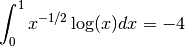
The program below computes this integral to a relative accuracy bound of
1e-7.
#include <stdio.h>
#include <math.h>
#include <gsl/gsl_integration.h>
double f (double x, void * params) {
double alpha = *(double *) params;
double f = log(alpha*x) / sqrt(x);
return f;
}
int
main (void)
{
gsl_integration_workspace * w
= gsl_integration_workspace_alloc (1000);
double result, error;
double expected = -4.0;
double alpha = 1.0;
gsl_function F;
F.function = &f;
F.params = α
gsl_integration_qags (&F, 0, 1, 0, 1e-7, 1000,
w, &result, &error);
printf ("result = % .18f\n", result);
printf ("exact result = % .18f\n", expected);
printf ("estimated error = % .18f\n", error);
printf ("actual error = % .18f\n", result - expected);
printf ("intervals = %zu\n", w->size);
gsl_integration_workspace_free (w);
return 0;
}
The results below show that the desired accuracy is achieved after 8 subdivisions.
result          = -4.000000000000085265
exact result    = -4.000000000000000000
estimated error =  0.000000000000135447
actual error    = -0.000000000000085265
intervals       = 8
In fact, the extrapolation procedure used by QAGS produces an
accuracy of almost twice as many digits. The error estimate returned by
the extrapolation procedure is larger than the actual error, giving a
margin of safety of one order of magnitude.
Fixed-point quadrature example
In this example, we use a fixed-point quadrature rule to integrate the integral
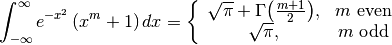
for integer . Consulting our table of fixed point quadratures,
we see that this integral can be evaluated with a Hermite quadrature rule,
setting  . Since we are integrating a polynomial
of degree , we need to choose the number of nodes
. Since we are integrating a polynomial
of degree , we need to choose the number of nodes  to achieve the best results.
First we will try integrating for  , which does not satisfy
our criteria above:
, which does not satisfy
our criteria above:
$ ./integration2 10 5
The output is,
m               = 10
intervals       = 5
result          =  47.468529694563351029
exact result    =  54.115231635459025483
actual error    = -6.646701940895674454
So, we find a large error. Now we try integrating for  which
does satisfy the criteria above:
which
does satisfy the criteria above:
$ ./integration2 10 6
The output is,
m               = 10
intervals       = 6
result          =  54.115231635459096537
exact result    =  54.115231635459025483
actual error    =  0.000000000000071054
The program is given below.
#include <stdio.h>
#include <math.h>
#include <gsl/gsl_integration.h>
#include <gsl/gsl_sf_gamma.h>

double
f(double x, void * params)
{
  int m = *(int *) params;
  double f = gsl_pow_int(x, m) + 1.0;
  return f;
}

int
main (int argc, char *argv[])
{
  gsl_integration_fixed_workspace * w;
  const gsl_integration_fixed_type * T = gsl_integration_fixed_hermite;
  int m = 10;
  int n = 6;
  double expected, result;
  gsl_function F;

  if (argc > 1)
    m = atoi(argv[1]);

  if (argc > 2)
    n = atoi(argv[2]);

  w = gsl_integration_fixed_alloc(T, n, 0.0, 1.0, 0.0, 0.0);

  F.function = &f;
  F.params = &m;

  gsl_integration_fixed(&F, &result, w);

  if (m % 2 == 0)
    expected = M_SQRTPI + gsl_sf_gamma(0.5*(1.0 + m));
  else
    expected = M_SQRTPI;

  printf ("m               = %d\n", m);
  printf ("intervals       = %zu\n", gsl_integration_fixed_n(w));
  printf ("result          = % .18f\n", result);
  printf ("exact result    = % .18f\n", expected);
  printf ("actual error    = % .18f\n", result - expected);

  gsl_integration_fixed_free (w);

  return 0;
}
References and Further Reading
The following book is the definitive reference for QUADPACK, and was written by the original authors. It provides descriptions of the algorithms, program listings, test programs and examples. It also includes useful advice on numerical integration and many references to the numerical integration literature used in developing QUADPACK.
R. Piessens, E. de Doncker-Kapenga, C.W. Ueberhuber, D.K. Kahaner. QUADPACK A subroutine package for automatic integration Springer Verlag, 1983.
The CQUAD integration algorithm is described in the following paper:
P. Gonnet, “Increasing the Reliability of Adaptive Quadrature Using Explicit Interpolants”, ACM Transactions on Mathematical Software, Volume 37 (2010), Issue 3, Article 26.
The fixed-point quadrature routines are based on IQPACK, described in the following papers:
S. Elhay, J. Kautsky, Algorithm 655: IQPACK, FORTRAN Subroutines for the Weights of Interpolatory Quadrature, ACM Transactions on Mathematical Software, Volume 13, Number 4, December 1987, pages 399-415.
J. Kautsky, S. Elhay, Calculation of the Weights of Interpolatory Quadratures, Numerische Mathematik, Volume 40, Number 3, October 1982, pages 407-422.
The Lebedev quadrature routines are based on the paper:
Lebedev, V. I. and Laikov, D. N. (1999). A quadrature formula for the sphere of the 131st algebraic order of accuracy. In Doklady Mathematics (Vol. 59, No. 3, pp. 477-481).