Polynomials¶

This chapter describes functions for evaluating and solving polynomials. There are routines for finding real and complex roots of quadratic and cubic equations using analytic methods. An iterative polynomial solver is also available for finding the roots of general polynomials with real coefficients (of any order). The functions are declared in the header file gsl_poly.h.

Polynomial Evaluation¶

The functions described here evaluate the polynomial

$P(x) = c[0] + c[1] x + c[2] x^2 + \dots + c[len-1] x^{len-1}$

using Horner’s method for stability. Inline versions of these functions are used when HAVE_INLINE is defined.

double gsl_poly_eval(const double c[], const int len, const double x)¶: This function evaluates a polynomial with real coefficients for the real variable x.

gsl_complex gsl_poly_complex_eval(const double c[], const int len, const gsl_complex z)¶: This function evaluates a polynomial with real coefficients for the complex variable z.

gsl_complex gsl_complex_poly_complex_eval(const gsl_complex c[], const int len, const gsl_complex z)¶: This function evaluates a polynomial with complex coefficients for the complex variable z.

int gsl_poly_eval_derivs(const double c[], const size_t lenc, const double x, double res[], const size_t lenres)¶: This function evaluates a polynomial and its derivatives storing the results in the array res of size lenres. The output array contains the values of $d^k P(x)/d x^k$ for the specified value of x starting with $k = 0$ .

Divided Difference Representation of Polynomials¶

The functions described here manipulate polynomials stored in Newton’s divided-difference representation. The use of divided-differences is described in Abramowitz & Stegun sections 25.1.4 and 25.2.26, and Burden and Faires, chapter 3, and discussed briefly below.

Given a function $f(x)$ , an $n$ th degree interpolating polynomial $P_{n}(x)$ can be constructed which agrees with $f$ at $n+1$ distinct points $x_0,x_1,...,x_{n}$ . This polynomial can be written in a form known as Newton’s divided-difference representation

$P_{n}(x) = f(x_0) + \sum_{k=1}^n [x_0,x_1,...,x_k] (x-x_0)(x-x_1) \cdots (x-x_{k-1})$

where the divided differences $[x_0,x_1,...,x_k]$ are defined in section 25.1.4 of Abramowitz and Stegun. Additionally, it is possible to construct an interpolating polynomial of degree $2n+1$ which also matches the first derivatives of $f$ at the points $x_0,x_1,...,x_n$ . This is called the Hermite interpolating polynomial and is defined as

$H_{2n+1}(x) = f(z_0) + \sum_{k=1}^{2n+1} [z_0,z_1,...,z_k] (x-z_0)(x-z_1) \cdots (x-z_{k-1})$

where the elements of $z = \{x_0,x_0,x_1,x_1,...,x_n,x_n\}$ are defined by $z_{2k} = z_{2k+1} = x_k$ . The divided-differences $[z_0,z_1,...,z_k]$ are discussed in Burden and Faires, section 3.4.

int gsl_poly_dd_init(double dd[], const double xa[], const double ya[], size_t size)¶: This function computes a divided-difference representation of the interpolating polynomial for the points $(x, y)$ stored in the arrays xa and ya of length size. On output the divided-differences of (xa, ya) are stored in the array dd, also of length size. Using the notation above, $dd[k] = [x_0,x_1,...,x_k]$ .

double gsl_poly_dd_eval(const double dd[], const double xa[], const size_t size, const double x)¶: This function evaluates the polynomial stored in divided-difference form in the arrays dd and xa of length size at the point x. An inline version of this function is used when HAVE_INLINE is defined.

int gsl_poly_dd_taylor(double c[], double xp, const double dd[], const double xa[], size_t size, double w[])¶: This function converts the divided-difference representation of a polynomial to a Taylor expansion. The divided-difference representation is supplied in the arrays dd and xa of length size. On output the Taylor coefficients of the polynomial expanded about the point xp are stored in the array c also of length size. A workspace of length size must be provided in the array w.

int gsl_poly_dd_hermite_init(double dd[], double za[], const double xa[], const double ya[], const double dya[], const size_t size)¶: This function computes a divided-difference representation of the interpolating Hermite polynomial for the points $(x,y)$ stored in the arrays xa and ya of length size. Hermite interpolation constructs polynomials which also match first derivatives $dy/dx$ which are provided in the array dya also of length size. The first derivatives can be incorported into the usual divided-difference algorithm by forming a new dataset $z = \{x_0,x_0,x_1,x_1,...\}$ , which is stored in the array za of length 2*size on output. On output the divided-differences of the Hermite representation are stored in the array dd, also of length 2*size. Using the notation above, $dd[k] = [z_0,z_1,...,z_k]$ . The resulting Hermite polynomial can be evaluated by calling gsl_poly_dd_eval() and using za for the input argument xa.

Quadratic Equations¶

int gsl_poly_solve_quadratic(double a, double b, double c, double *x0, double *x1)¶

This function finds the real roots of the quadratic equation,

$a x^2 + b x + c = 0$

The number of real roots (either zero, one or two) is returned, and their locations are stored in x0 and x1. If no real roots are found then x0 and x1 are not modified. If one real root is found (i.e. if $a=0$ ) then it is stored in x0. When two real roots are found they are stored in x0 and x1 in ascending order. The case of coincident roots is not considered special. For example $(x-1)^2=0$ will have two roots, which happen to have exactly equal values.

The number of roots found depends on the sign of the discriminant $b^2 - 4 a c$ . This will be subject to rounding and cancellation errors when computed in double precision, and will also be subject to errors if the coefficients of the polynomial are inexact. These errors may cause a discrete change in the number of roots. However, for polynomials with small integer coefficients the discriminant can always be computed exactly.

int gsl_poly_complex_solve_quadratic(double a, double b, double c, gsl_complex *z0, gsl_complex *z1)¶

This function finds the complex roots of the quadratic equation,

$a z^2 + b z + c = 0$

The number of complex roots is returned (either one or two) and the locations of the roots are stored in z0 and z1. The roots are returned in ascending order, sorted first by their real components and then by their imaginary components. If only one real root is found (i.e. if $a=0$ ) then it is stored in z0.

Cubic Equations¶

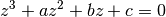
int gsl_poly_solve_cubic(double a, double b, double c, double *x0, double *x1, double *x2)¶

This function finds the real roots of the cubic equation,

$x^3 + a x^2 + b x + c = 0$

with a leading coefficient of unity. The number of real roots (either one or three) is returned, and their locations are stored in x0, x1 and x2. If one real root is found then only x0 is modified. When three real roots are found they are stored in x0, x1 and x2 in ascending order. The case of coincident roots is not considered special. For example, the equation $(x-1)^3=0$ will have three roots with exactly equal values. As in the quadratic case, finite precision may cause equal or closely-spaced real roots to move off the real axis into the complex plane, leading to a discrete change in the number of real roots.

int gsl_poly_complex_solve_cubic(double a, double b, double c, gsl_complex *z0, gsl_complex *z1, gsl_complex *z2)¶

This function finds the complex roots of the cubic equation,

$z^3 + a z^2 + b z + c = 0$

The number of complex roots is returned (always three) and the locations of the roots are stored in z0, z1 and z2. The roots are returned in ascending order, sorted first by their real components and then by their imaginary components.

General Polynomial Equations¶

The roots of polynomial equations cannot be found analytically beyond the special cases of the quadratic, cubic and quartic equation. The algorithm described in this section uses an iterative method to find the approximate locations of roots of higher order polynomials.

type gsl_poly_complex_workspace¶: This workspace contains parameters used for finding roots of general polynomials

gsl_poly_complex_workspace *gsl_poly_complex_workspace_alloc(size_t n)¶

This function allocates space for a gsl_poly_complex_workspace struct and a workspace suitable for solving a polynomial with n coefficients using the routine gsl_poly_complex_solve().

The function returns a pointer to the newly allocated gsl_poly_complex_workspace if no errors were detected, and a null pointer in the case of error.

void gsl_poly_complex_workspace_free(gsl_poly_complex_workspace *w)¶: This function frees all the memory associated with the workspace w.

int gsl_poly_complex_solve(const double *a, size_t n, gsl_poly_complex_workspace *w, gsl_complex_packed_ptr z)¶

This function computes the roots of the general polynomial

$P(x) = a_0 + a_1 x + a_2 x^2 + \cdots + a_{n-1} x^{n-1}$

using balanced-QR reduction of the companion matrix. The parameter n specifies the length of the coefficient array. The coefficient of the highest order term must be non-zero. The function requires a workspace w of the appropriate size. The $n-1$ roots are returned in the packed complex array z of length $2(n-1)$ , alternating real and imaginary parts.

The function returns GSL_SUCCESS if all the roots are found. If the QR reduction does not converge, the error handler is invoked with an error code of GSL_EFAILED. Note that due to finite precision, roots of higher multiplicity are returned as a cluster of simple roots with reduced accuracy. The solution of polynomials with higher-order roots requires specialized algorithms that take the multiplicity structure into account (see e.g. Z. Zeng, Algorithm 835, ACM Transactions on Mathematical Software, Volume 30, Issue 2 (2004), pp 218–236).

Examples¶

To demonstrate the use of the general polynomial solver we will take the polynomial 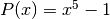$P(x) = x^5 - 1$ which has these roots:

$1, e^{2\pi i / 5}, e^{4\pi i / 5}, e^{6\pi i / 5}, e^{8\pi i / 5}$

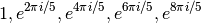
The following program will find these roots.

#include <stdio.h>
#include <gsl/gsl_poly.h>

int
main (void)
{
  int i;
  /* coefficients of P(x) =  -1 + x^5  */
  double a[6] = { -1, 0, 0, 0, 0, 1 };
  double z[10];

  gsl_poly_complex_workspace * w
      = gsl_poly_complex_workspace_alloc (6);

  gsl_poly_complex_solve (a, 6, w, z);

  gsl_poly_complex_workspace_free (w);

  for (i = 0; i < 5; i++)
    {
      printf ("z%d = %+.18f %+.18f\n",
              i, z[2*i], z[2*i+1]);
    }

  return 0;
}

The output of the program is

z0 = -0.809016994374947673 +0.587785252292473359
z1 = -0.809016994374947673 -0.587785252292473359
z2 = +0.309016994374947507 +0.951056516295152976
z3 = +0.309016994374947507 -0.951056516295152976
z4 = +0.999999999999999889 +0.000000000000000000

which agrees with the analytic result, 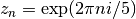$z_n = \exp(2 \pi n i/5)$ .

References and Further Reading¶

The balanced-QR method and its error analysis are described in the following papers,

R.S. Martin, G. Peters and J.H. Wilkinson, “The QR Algorithm for Real Hessenberg Matrices”, Numerische Mathematik, 14 (1970), 219–231.
B.N. Parlett and C. Reinsch, “Balancing a Matrix for Calculation of Eigenvalues and Eigenvectors”, Numerische Mathematik, 13 (1969), 293–304.
A. Edelman and H. Murakami, “Polynomial roots from companion matrix eigenvalues”, Mathematics of Computation, Vol.: 64, No.: 210 (1995), 763–776.

The formulas for divided differences are given in the following texts,

Abramowitz and Stegun, Handbook of Mathematical Functions, Sections 25.1.4 and 25.2.26.
R. L. Burden and J. D. Faires, Numerical Analysis, 9th edition, ISBN 0-538-73351-9, 2011.