Sparse Linear Algebra
This chapter describes functions for solving sparse linear systems
of equations. The library provides linear algebra routines which
operate directly on the gsl_spmatrix and gsl_vector
objects.
The functions described in this chapter are declared in the header file
gsl_splinalg.h.
Overview
This chapter is primarily concerned with the solution of the linear system

where  is a general square
  -by- non-singular
sparse matrix,
-by- non-singular
sparse matrix,  is an unknown -by-
 vector, and
 is a given -by-1 right hand side vector. There exist
many methods for solving such sparse linear systems, which broadly
fall into either direct or iterative categories. Direct methods include
LU and QR decompositions, while iterative methods start with an
initial guess for the vector and update the guess through
iteration until convergence. GSL does not currently provide any
direct sparse solvers.
is a given -by-1 right hand side vector. There exist
many methods for solving such sparse linear systems, which broadly
fall into either direct or iterative categories. Direct methods include
LU and QR decompositions, while iterative methods start with an
initial guess for the vector and update the guess through
iteration until convergence. GSL does not currently provide any
direct sparse solvers.
Sparse Iterative Solvers
Overview
Many practical iterative methods of solving large -by-
sparse linear systems involve projecting an approximate solution for
x onto a subspace of  . If we define a
  -dimensional
subspace
-dimensional
subspace  as the subspace of approximations to the solution
x, then constraints must be imposed to determine
the next approximation. These constraints define another
-dimensional subspace denoted by  . The
subspace dimension is typically chosen to be much smaller than
in order to reduce the computational
effort needed to generate the next approximate solution vector.
The many iterative algorithms which exist differ mainly
in their choice of and .
. The
subspace dimension is typically chosen to be much smaller than
in order to reduce the computational
effort needed to generate the next approximate solution vector.
The many iterative algorithms which exist differ mainly
in their choice of and .
Types of Sparse Iterative Solvers
The sparse linear algebra library provides the following types of iterative solvers:
-
type gsl_splinalg_itersolve_type
-
gsl_splinalg_itersolve_type *gsl_splinalg_itersolve_gmres
This specifies the Generalized Minimum Residual Method (GMRES). This is a projection method using
 and
and  where
where  is
the -th Krylov subspace
is
the -th Krylov subspace
and
 is the residual vector of the initial guess
 . If is set equal to , then the Krylov
subspace is and GMRES will provide the exact solution
. If is set equal to , then the Krylov
subspace is and GMRES will provide the exact solution
x. However, the goal is for the method to arrive at a very good approximation toxusing a much smaller subspace. By
default, the GMRES method selects  but the user
may specify a different value for . The GMRES storage
requirements grow as
but the user
may specify a different value for . The GMRES storage
requirements grow as  and the number of flops
grow as
and the number of flops
grow as  .
.In the below function
gsl_splinalg_itersolve_iterate(), one GMRES iteration is defined as projecting the approximate solution vector onto each Krylov subspace ,
and so can be kept smaller by “restarting” the method
and calling
,
and so can be kept smaller by “restarting” the method
and calling gsl_splinalg_itersolve_iterate()multiple times, providing the updated approximationxto each new call. If the method is not adequately converging, the user may try increasing the parameter.GMRES is considered a robust general purpose iterative solver, however there are cases where the method stagnates if the matrix is not positive-definite and fails to reduce the residual until the very last projection onto the subspace
 . In these
cases, preconditioning the linear system can help, but GSL does not
currently provide any preconditioners.
. In these
cases, preconditioning the linear system can help, but GSL does not
currently provide any preconditioners.
-
gsl_splinalg_itersolve_type *gsl_splinalg_itersolve_gmres
Iterating the Sparse Linear System
The following functions are provided to allocate storage for the sparse linear solvers and iterate the system to a solution.
-
gsl_splinalg_itersolve *gsl_splinalg_itersolve_alloc(const gsl_splinalg_itersolve_type *T, const size_t n, const size_t m)
This function allocates a workspace for the iterative solution of
n-by-nsparse matrix systems. The iterative solver type is specified byT. The argumentmspecifies the size of the solution candidate subspace. The dimension
mmay be set to 0 in which case a reasonable default value is used.
-
void gsl_splinalg_itersolve_free(gsl_splinalg_itersolve *w)
This function frees the memory associated with the workspace
w.
-
const char *gsl_splinalg_itersolve_name(const gsl_splinalg_itersolve *w)
This function returns a string pointer to the name of the solver.
-
int gsl_splinalg_itersolve_iterate(const gsl_spmatrix *A, const gsl_vector *b, const double tol, gsl_vector *x, gsl_splinalg_itersolve *w)
This function performs one iteration of the iterative method for the sparse linear system specfied by the matrix
A, right hand side vectorband solution vectorx. On input,xmust be set to an initial guess for the solution. On output,xis updated to give the current solution estimate. The parametertolspecifies the relative tolerance between the residual norm and norm ofbin order to check for convergence. When the following condition is satisfied:
the method has converged, the function returns
GSL_SUCCESSand the final solution is provided inx. Otherwise, the function returnsGSL_CONTINUEto signal that more iterations are required. Here, represents the Euclidean norm.
The input matrix
represents the Euclidean norm.
The input matrix Amay be in triplet or compressed format.
-
double gsl_splinalg_itersolve_normr(const gsl_splinalg_itersolve *w)
This function returns the current residual norm
 , which is updated after each call to
gsl_splinalg_itersolve_iterate().
Examples
This example program demonstrates the sparse linear algebra routines on
the solution of a simple 1D Poisson equation on ![[0,1]](_images/math/e7e8ac4ddd4ab0fc62c2a6435f8373f48c776858.png) :
:
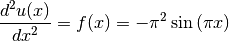
with boundary conditions 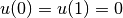 . The analytic solution of
this simple problem is
. The analytic solution of
this simple problem is 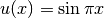 . We will solve this
problem by finite differencing the left hand side to give
. We will solve this
problem by finite differencing the left hand side to give
Defining a grid of  points,
  . In the finite
difference equation above,
. In the finite
difference equation above,  are known from
the boundary conditions, so we will only put the equations for
are known from
the boundary conditions, so we will only put the equations for
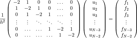
 into the matrix system. The resulting
 matrix equation is
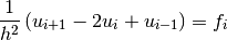
An example program which constructs and solves this system is given below. The system is solved using the iterative GMRES solver. Here is the output of the program:
iter 0 residual = 4.297275996844e-11
Converged
showing that the method converged in a single iteration. The calculated solution is shown in Fig. 50.

Fig. 50 Solution of PDE
#include <stdio.h>
#include <stdlib.h>
#include <math.h>

#include <gsl/gsl_math.h>
#include <gsl/gsl_vector.h>
#include <gsl/gsl_spmatrix.h>
#include <gsl/gsl_splinalg.h>

int
main()
{
  const size_t N = 100;                       /* number of grid points */
  const size_t n = N - 2;                     /* subtract 2 to exclude boundaries */
  const double h = 1.0 / (N - 1.0);           /* grid spacing */
  gsl_spmatrix *A = gsl_spmatrix_alloc(n ,n); /* triplet format */
  gsl_spmatrix *C;                            /* compressed format */
  gsl_vector *f = gsl_vector_alloc(n);        /* right hand side vector */
  gsl_vector *u = gsl_vector_alloc(n);        /* solution vector */
  size_t i;

  /* construct the sparse matrix for the finite difference equation */

  /* construct first row */
  gsl_spmatrix_set(A, 0, 0, -2.0);
  gsl_spmatrix_set(A, 0, 1, 1.0);

  /* construct rows [1:n-2] */
  for (i = 1; i < n - 1; ++i)
    {
      gsl_spmatrix_set(A, i, i + 1, 1.0);
      gsl_spmatrix_set(A, i, i, -2.0);
      gsl_spmatrix_set(A, i, i - 1, 1.0);
    }

  /* construct last row */
  gsl_spmatrix_set(A, n - 1, n - 1, -2.0);
  gsl_spmatrix_set(A, n - 1, n - 2, 1.0);

  /* scale by h^2 */
  gsl_spmatrix_scale(A, 1.0 / (h * h));

  /* construct right hand side vector */
  for (i = 0; i < n; ++i)
    {
      double xi = (i + 1) * h;
      double fi = -M_PI * M_PI * sin(M_PI * xi);
      gsl_vector_set(f, i, fi);
    }

  /* convert to compressed column format */
  C = gsl_spmatrix_ccs(A);

  /* now solve the system with the GMRES iterative solver */
  {
    const double tol = 1.0e-6;  /* solution relative tolerance */
    const size_t max_iter = 10; /* maximum iterations */
    const gsl_splinalg_itersolve_type *T = gsl_splinalg_itersolve_gmres;
    gsl_splinalg_itersolve *work =
      gsl_splinalg_itersolve_alloc(T, n, 0);
    size_t iter = 0;
    double residual;
    int status;

    /* initial guess u = 0 */
    gsl_vector_set_zero(u);

    /* solve the system A u = f */
    do
      {
        status = gsl_splinalg_itersolve_iterate(C, f, tol, u, work);

        /* print out residual norm ||A*u - f|| */
        residual = gsl_splinalg_itersolve_normr(work);
        fprintf(stderr, "iter %zu residual = %.12e\n", iter, residual);

        if (status == GSL_SUCCESS)
          fprintf(stderr, "Converged\n");
      }
    while (status == GSL_CONTINUE && ++iter < max_iter);

    /* output solution */
    for (i = 0; i < n; ++i)
      {
        double xi = (i + 1) * h;
        double u_exact = sin(M_PI * xi);
        double u_gsl = gsl_vector_get(u, i);

        printf("%f %.12e %.12e\n", xi, u_gsl, u_exact);
      }

    gsl_splinalg_itersolve_free(work);
  }

  gsl_spmatrix_free(A);
  gsl_spmatrix_free(C);
  gsl_vector_free(f);
  gsl_vector_free(u);

  return 0;
} /* main() */
References and Further Reading
The implementation of the GMRES iterative solver closely follows the publications
H. F. Walker, Implementation of the GMRES method using Householder transformations, SIAM J. Sci. Stat. Comput. 9(1), 1988.
Y. Saad, Iterative methods for sparse linear systems, 2nd edition, SIAM, 2003.