Special Functions
This chapter describes the GSL special function library. The library includes routines for calculating the values of Airy functions, Bessel functions, Clausen functions, Coulomb wave functions, Coupling coefficients, the Dawson function, Debye functions, Dilogarithms, Elliptic integrals, Jacobi elliptic functions, Error functions, Exponential integrals, Fermi-Dirac functions, Gamma functions, Gegenbauer functions, Hermite polynomials and functions, Hypergeometric functions, Laguerre functions, Legendre functions and Spherical Harmonics, the Psi (Digamma) Function, Synchrotron functions, Transport functions, Trigonometric functions and Zeta functions. Each routine also computes an estimate of the numerical error in the calculated value of the function.
The functions in this chapter are declared in individual header files,
such as gsl_sf_airy.h, gsl_sf_bessel.h, etc. The complete
set of header files can be included using the file gsl_sf.h.
Usage
The special functions are available in two calling conventions, a natural form which returns the numerical value of the function and an error-handling form which returns an error code. The two types of function provide alternative ways of accessing the same underlying code.
The natural form returns only the value of the function and can be
used directly in mathematical expressions. For example, the following
function call will compute the value of the Bessel function
 :
:
double y = gsl_sf_bessel_J0 (x);
There is no way to access an error code or to estimate the error using this method. To allow access to this information the alternative error-handling form stores the value and error in a modifiable argument:
gsl_sf_result result;
int status = gsl_sf_bessel_J0_e (x, &result);
The error-handling functions have the suffix _e. The returned
status value indicates error conditions such as overflow, underflow or
loss of precision. If there are no errors the error-handling functions
return GSL_SUCCESS.
The gsl_sf_result struct
The error handling form of the special functions always calculate an
error estimate along with the value of the result. Therefore,
structures are provided for amalgamating a value and error estimate.
These structures are declared in the header file gsl_sf_result.h.
The following struct contains value and error fields.
-
type gsl_sf_result
typedef struct
{
  double val;
  double err;
} gsl_sf_result;
The field
valcontains the value and the fielderrcontains an estimate of the absolute error in the value.
In some cases, an overflow or underflow can be detected and handled by a
function. In this case, it may be possible to return a scaling exponent
as well as an error/value pair in order to save the result from
exceeding the dynamic range of the built-in types. The
following struct contains value and error fields as well
as an exponent field such that the actual result is obtained as
result * 10^(e10).
-
type gsl_sf_result_e10
typedef struct
{
  double val;
  double err;
  int    e10;
} gsl_sf_result_e10;
Modes
The goal of the library is to achieve double precision accuracy wherever
possible. However the cost of evaluating some special functions to
double precision can be significant, particularly where very high order
terms are required. In these cases a mode argument, of type
gsl_mode_t allows the
accuracy of the function to be reduced in order to improve performance.
The following precision levels are available for the mode argument,
-
type gsl_mode_t
-
GSL_PREC_DOUBLE
Double-precision, a relative accuracy of approximately
 .
.
-
GSL_PREC_SINGLE
Single-precision, a relative accuracy of approximately
 .
.
-
GSL_PREC_APPROX
Approximate values, a relative accuracy of approximately
 .
.
-
GSL_PREC_DOUBLE
The approximate mode provides the fastest evaluation at the lowest accuracy.
Airy Functions and Derivatives
The Airy functions  and
and  are defined by the
integral representations,
are defined by the
integral representations,
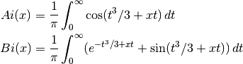
For further information see Abramowitz & Stegun, Section 10.4. The Airy
functions are defined in the header file gsl_sf_airy.h.
Airy Functions
-
double gsl_sf_airy_Ai(double x, gsl_mode_t mode)
-
int gsl_sf_airy_Ai_e(double x, gsl_mode_t mode, gsl_sf_result *result)
These routines compute the Airy function
with an accuracy
specified by mode.
-
double gsl_sf_airy_Bi(double x, gsl_mode_t mode)
-
int gsl_sf_airy_Bi_e(double x, gsl_mode_t mode, gsl_sf_result *result)
These routines compute the Airy function
with an accuracy
specified by mode.
-
double gsl_sf_airy_Ai_scaled(double x, gsl_mode_t mode)
-
int gsl_sf_airy_Ai_scaled_e(double x, gsl_mode_t mode, gsl_sf_result *result)
These routines compute a scaled version of the Airy function
 . For
. For  the scaling factor
  is
is
 ,
and is 1 for
,
and is 1 for  .
.
-
double gsl_sf_airy_Bi_scaled(double x, gsl_mode_t mode)
-
int gsl_sf_airy_Bi_scaled_e(double x, gsl_mode_t mode, gsl_sf_result *result)
These routines compute a scaled version of the Airy function
 . For the scaling factor
  is
is
 , and is 1 for .
Derivatives of Airy Functions
-
double gsl_sf_airy_Ai_deriv(double x, gsl_mode_t mode)
-
int gsl_sf_airy_Ai_deriv_e(double x, gsl_mode_t mode, gsl_sf_result *result)
These routines compute the Airy function derivative
 with
an accuracy specified by
with
an accuracy specified by mode.
-
double gsl_sf_airy_Bi_deriv(double x, gsl_mode_t mode)
-
int gsl_sf_airy_Bi_deriv_e(double x, gsl_mode_t mode, gsl_sf_result *result)
These routines compute the Airy function derivative
 with
an accuracy specified by
with
an accuracy specified by mode.
-
double gsl_sf_airy_Ai_deriv_scaled(double x, gsl_mode_t mode)
-
int gsl_sf_airy_Ai_deriv_scaled_e(double x, gsl_mode_t mode, gsl_sf_result *result)
These routines compute the scaled Airy function derivative
 .
For the scaling factor is
, and is 1 for .
.
For the scaling factor is
, and is 1 for .
-
double gsl_sf_airy_Bi_deriv_scaled(double x, gsl_mode_t mode)
-
int gsl_sf_airy_Bi_deriv_scaled_e(double x, gsl_mode_t mode, gsl_sf_result *result)
These routines compute the scaled Airy function derivative
 .
For the scaling factor is
, and is 1 for .
.
For the scaling factor is
, and is 1 for .
Zeros of Airy Functions
-
double gsl_sf_airy_zero_Ai(unsigned int s)
-
int gsl_sf_airy_zero_Ai_e(unsigned int s, gsl_sf_result *result)
These routines compute the location of the
s-th zero of the Airy function.
-
double gsl_sf_airy_zero_Bi(unsigned int s)
-
int gsl_sf_airy_zero_Bi_e(unsigned int s, gsl_sf_result *result)
These routines compute the location of the
s-th zero of the Airy function.
Zeros of Derivatives of Airy Functions
-
double gsl_sf_airy_zero_Ai_deriv(unsigned int s)
-
int gsl_sf_airy_zero_Ai_deriv_e(unsigned int s, gsl_sf_result *result)
These routines compute the location of the
s-th zero of the Airy function derivative.
-
double gsl_sf_airy_zero_Bi_deriv(unsigned int s)
-
int gsl_sf_airy_zero_Bi_deriv_e(unsigned int s, gsl_sf_result *result)
These routines compute the location of the
s-th zero of the Airy function derivative.
Bessel Functions
The routines described in this section compute the Cylindrical Bessel
functions  ,
,  , Modified cylindrical Bessel
functions
, Modified cylindrical Bessel
functions  ,
,  , Spherical Bessel functions
 ,
,  , and Modified Spherical Bessel functions
 ,
,  . For more information see Abramowitz & Stegun,
Chapters 9 and 10. The Bessel functions are defined in the header file
. For more information see Abramowitz & Stegun,
Chapters 9 and 10. The Bessel functions are defined in the header file
gsl_sf_bessel.h.
Regular Cylindrical Bessel Functions
-
double gsl_sf_bessel_J0(double x)
-
int gsl_sf_bessel_J0_e(double x, gsl_sf_result *result)
These routines compute the regular cylindrical Bessel function of zeroth order,
.
-
double gsl_sf_bessel_J1(double x)
-
int gsl_sf_bessel_J1_e(double x, gsl_sf_result *result)
These routines compute the regular cylindrical Bessel function of first order,
 .
.
-
double gsl_sf_bessel_Jn(int n, double x)
-
int gsl_sf_bessel_Jn_e(int n, double x, gsl_sf_result *result)
These routines compute the regular cylindrical Bessel function of order
n,.
-
int gsl_sf_bessel_Jn_array(int nmin, int nmax, double x, double result_array[])
This routine computes the values of the regular cylindrical Bessel functions
for  from
from nmintonmaxinclusive, storing the results in the arrayresult_array. The values are computed using recurrence relations for efficiency, and therefore may differ slightly from the exact values.
Irregular Cylindrical Bessel Functions
-
double gsl_sf_bessel_Y0(double x)
-
int gsl_sf_bessel_Y0_e(double x, gsl_sf_result *result)
These routines compute the irregular cylindrical Bessel function of zeroth order,
 , for
, for  .
.
-
double gsl_sf_bessel_Y1(double x)
-
int gsl_sf_bessel_Y1_e(double x, gsl_sf_result *result)
These routines compute the irregular cylindrical Bessel function of first order,
 , for .
-
double gsl_sf_bessel_Yn(int n, double x)
-
int gsl_sf_bessel_Yn_e(int n, double x, gsl_sf_result *result)
These routines compute the irregular cylindrical Bessel function of order
n,, for .
-
int gsl_sf_bessel_Yn_array(int nmin, int nmax, double x, double result_array[])
This routine computes the values of the irregular cylindrical Bessel functions
for from nmintonmaxinclusive, storing the results in the arrayresult_array. The domain of the function is. The values are computed using
recurrence relations for efficiency, and therefore may differ slightly
from the exact values.
Regular Modified Cylindrical Bessel Functions
-
double gsl_sf_bessel_I0(double x)
-
int gsl_sf_bessel_I0_e(double x, gsl_sf_result *result)
These routines compute the regular modified cylindrical Bessel function of zeroth order,
 .
.
-
double gsl_sf_bessel_I1(double x)
-
int gsl_sf_bessel_I1_e(double x, gsl_sf_result *result)
These routines compute the regular modified cylindrical Bessel function of first order,
 .
.
-
double gsl_sf_bessel_In(int n, double x)
-
int gsl_sf_bessel_In_e(int n, double x, gsl_sf_result *result)
These routines compute the regular modified cylindrical Bessel function of order
n,.
-
int gsl_sf_bessel_In_array(int nmin, int nmax, double x, double result_array[])
This routine computes the values of the regular modified cylindrical Bessel functions
for from nmintonmaxinclusive, storing the results in the arrayresult_array. The start of the rangenminmust be positive or zero. The values are computed using recurrence relations for efficiency, and therefore may differ slightly from the exact values.
-
double gsl_sf_bessel_I0_scaled(double x)
-
int gsl_sf_bessel_I0_scaled_e(double x, gsl_sf_result *result)
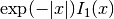
These routines compute the scaled regular modified cylindrical Bessel function of zeroth order
 .
.
-
double gsl_sf_bessel_I1_scaled(double x)
-
int gsl_sf_bessel_I1_scaled_e(double x, gsl_sf_result *result)
These routines compute the scaled regular modified cylindrical Bessel function of first order
 .
.
-
double gsl_sf_bessel_In_scaled(int n, double x)
-
int gsl_sf_bessel_In_scaled_e(int n, double x, gsl_sf_result *result)
These routines compute the scaled regular modified cylindrical Bessel function of order
n,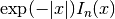
-
int gsl_sf_bessel_In_scaled_array(int nmin, int nmax, double x, double result_array[])
This routine computes the values of the scaled regular cylindrical Bessel functions
for from
nmintonmaxinclusive, storing the results in the arrayresult_array. The start of the rangenminmust be positive or zero. The values are computed using recurrence relations for efficiency, and therefore may differ slightly from the exact values.
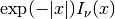
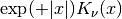
Irregular Modified Cylindrical Bessel Functions
-
double gsl_sf_bessel_K0(double x)
-
int gsl_sf_bessel_K0_e(double x, gsl_sf_result *result)
These routines compute the irregular modified cylindrical Bessel function of zeroth order,
 , for .
-
double gsl_sf_bessel_K1(double x)
-
int gsl_sf_bessel_K1_e(double x, gsl_sf_result *result)
These routines compute the irregular modified cylindrical Bessel function of first order,
 , for .
-
double gsl_sf_bessel_Kn(int n, double x)
-
int gsl_sf_bessel_Kn_e(int n, double x, gsl_sf_result *result)
These routines compute the irregular modified cylindrical Bessel function of order
n,, for .
-
int gsl_sf_bessel_Kn_array(int nmin, int nmax, double x, double result_array[])
This routine computes the values of the irregular modified cylindrical Bessel functions
for from nmintonmaxinclusive, storing the results in the arrayresult_array. The start of the rangenminmust be positive or zero. The domain of the function is. The values are
computed using recurrence relations for efficiency, and therefore
may differ slightly from the exact values.
-
double gsl_sf_bessel_K0_scaled(double x)
-
int gsl_sf_bessel_K0_scaled_e(double x, gsl_sf_result *result)
These routines compute the scaled irregular modified cylindrical Bessel function of zeroth order
 for .
for .
-
double gsl_sf_bessel_K1_scaled(double x)
-
int gsl_sf_bessel_K1_scaled_e(double x, gsl_sf_result *result)
These routines compute the scaled irregular modified cylindrical Bessel function of first order
 for .
for .
-
double gsl_sf_bessel_Kn_scaled(int n, double x)
-
int gsl_sf_bessel_Kn_scaled_e(int n, double x, gsl_sf_result *result)
These routines compute the scaled irregular modified cylindrical Bessel function of order
n, , for .
-
int gsl_sf_bessel_Kn_scaled_array(int nmin, int nmax, double x, double result_array[])
This routine computes the values of the scaled irregular cylindrical Bessel functions
for from nmintonmaxinclusive, storing the results in the arrayresult_array. The start of the rangenminmust be positive or zero. The domain of the function is. The values are
computed using recurrence relations for efficiency, and therefore
may differ slightly from the exact values.
Regular Spherical Bessel Functions
-
double gsl_sf_bessel_j0(double x)
-
int gsl_sf_bessel_j0_e(double x, gsl_sf_result *result)
These routines compute the regular spherical Bessel function of zeroth order,
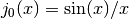 .
.
-
double gsl_sf_bessel_j1(double x)
-
int gsl_sf_bessel_j1_e(double x, gsl_sf_result *result)
These routines compute the regular spherical Bessel function of first order,
 .
.
-
double gsl_sf_bessel_j2(double x)
-
int gsl_sf_bessel_j2_e(double x, gsl_sf_result *result)
These routines compute the regular spherical Bessel function of second order,
 .
.
-
double gsl_sf_bessel_jl(int l, double x)
-
int gsl_sf_bessel_jl_e(int l, double x, gsl_sf_result *result)
These routines compute the regular spherical Bessel function of order
l,, for
 and
and  .
.
-
int gsl_sf_bessel_jl_array(int lmax, double x, double result_array[])
This routine computes the values of the regular spherical Bessel functions
for  from 0 to
 lmaxinclusive for and
, storing the results in the array
and
, storing the results in the array result_array. The values are computed using recurrence relations for efficiency, and therefore may differ slightly from the exact values.
-
int gsl_sf_bessel_jl_steed_array(int lmax, double x, double *result_array)
This routine uses Steed’s method to compute the values of the regular spherical Bessel functions
for from 0 to
lmaxinclusive for and
, storing the results in the array
result_array. The Steed/Barnett algorithm is described in Comp. Phys. Comm. 21, 297 (1981). Steed’s method is more stable than the recurrence used in the other functions but is also slower.
Irregular Spherical Bessel Functions
-
double gsl_sf_bessel_y0(double x)
-
int gsl_sf_bessel_y0_e(double x, gsl_sf_result *result)
These routines compute the irregular spherical Bessel function of zeroth order,
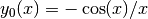 .
.
-
double gsl_sf_bessel_y1(double x)
-
int gsl_sf_bessel_y1_e(double x, gsl_sf_result *result)
These routines compute the irregular spherical Bessel function of first order,
 .
.
-
double gsl_sf_bessel_y2(double x)
-
int gsl_sf_bessel_y2_e(double x, gsl_sf_result *result)
These routines compute the irregular spherical Bessel function of second order,
 .
.
-
double gsl_sf_bessel_yl(int l, double x)
-
int gsl_sf_bessel_yl_e(int l, double x, gsl_sf_result *result)
These routines compute the irregular spherical Bessel function of order
l,, for
.
-
int gsl_sf_bessel_yl_array(int lmax, double x, double result_array[])
This routine computes the values of the irregular spherical Bessel functions
for from 0 to lmaxinclusive for, storing the results in the array result_array. The values are computed using recurrence relations for efficiency, and therefore may differ slightly from the exact values.
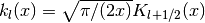
Regular Modified Spherical Bessel Functions
The regular modified spherical Bessel functions
are related to the modified Bessel functions of fractional order,
-
double gsl_sf_bessel_i0_scaled(double x)
-
int gsl_sf_bessel_i0_scaled_e(double x, gsl_sf_result *result)
These routines compute the scaled regular modified spherical Bessel function of zeroth order,
 .
.
-
double gsl_sf_bessel_i1_scaled(double x)
-
int gsl_sf_bessel_i1_scaled_e(double x, gsl_sf_result *result)
These routines compute the scaled regular modified spherical Bessel function of first order,
 .
.
-
double gsl_sf_bessel_i2_scaled(double x)
-
int gsl_sf_bessel_i2_scaled_e(double x, gsl_sf_result *result)
These routines compute the scaled regular modified spherical Bessel function of second order,
-
double gsl_sf_bessel_il_scaled(int l, double x)
-
int gsl_sf_bessel_il_scaled_e(int l, double x, gsl_sf_result *result)
These routines compute the scaled regular modified spherical Bessel function of order
l,
-
int gsl_sf_bessel_il_scaled_array(int lmax, double x, double result_array[])
This routine computes the values of the scaled regular modified spherical Bessel functions
for from
0 to lmaxinclusive for, storing the results in
the array result_array. The values are computed using recurrence relations for efficiency, and therefore may differ slightly from the exact values.
Irregular Modified Spherical Bessel Functions
The irregular modified spherical Bessel functions
are related to the irregular modified Bessel functions of fractional order,
 .
.
-
double gsl_sf_bessel_k0_scaled(double x)
-
int gsl_sf_bessel_k0_scaled_e(double x, gsl_sf_result *result)
These routines compute the scaled irregular modified spherical Bessel function of zeroth order,
 , for .
-
double gsl_sf_bessel_k1_scaled(double x)
-
int gsl_sf_bessel_k1_scaled_e(double x, gsl_sf_result *result)
These routines compute the scaled irregular modified spherical Bessel function of first order,
 , for .
-
double gsl_sf_bessel_k2_scaled(double x)
-
int gsl_sf_bessel_k2_scaled_e(double x, gsl_sf_result *result)
These routines compute the scaled irregular modified spherical Bessel function of second order,
 , for .
-
double gsl_sf_bessel_kl_scaled(int l, double x)
-
int gsl_sf_bessel_kl_scaled_e(int l, double x, gsl_sf_result *result)
These routines compute the scaled irregular modified spherical Bessel function of order
l, , for .
-
int gsl_sf_bessel_kl_scaled_array(int lmax, double x, double result_array[])
This routine computes the values of the scaled irregular modified spherical Bessel functions
for from
0 to lmaxinclusive for and , storing the results in
the array result_array. The values are computed using recurrence relations for efficiency, and therefore may differ slightly from the exact values.
Regular Bessel Function—Fractional Order
-
double gsl_sf_bessel_Jnu(double nu, double x)
-
int gsl_sf_bessel_Jnu_e(double nu, double x, gsl_sf_result *result)
These routines compute the regular cylindrical Bessel function of fractional order
 ,
,  .
.
-
int gsl_sf_bessel_sequence_Jnu_e(double nu, gsl_mode_t mode, size_t size, double v[])
This function computes the regular cylindrical Bessel function of fractional order
, , evaluated at a series of
 values. The array
 vof lengthsizecontains the values. They are assumed to be strictly ordered and positive.
The array is over-written with the values of  .
.
Irregular Bessel Functions—Fractional Order
-
double gsl_sf_bessel_Ynu(double nu, double x)
-
int gsl_sf_bessel_Ynu_e(double nu, double x, gsl_sf_result *result)
These routines compute the irregular cylindrical Bessel function of fractional order
,  .
.
Regular Modified Bessel Functions—Fractional Order
-
double gsl_sf_bessel_Inu(double nu, double x)
-
int gsl_sf_bessel_Inu_e(double nu, double x, gsl_sf_result *result)
These routines compute the regular modified Bessel function of fractional order
,  for ,
for ,
 .
.
-
double gsl_sf_bessel_Inu_scaled(double nu, double x)
-
int gsl_sf_bessel_Inu_scaled_e(double nu, double x, gsl_sf_result *result)
These routines compute the scaled regular modified Bessel function of fractional order
,  for ,
.
for ,
.
Irregular Modified Bessel Functions—Fractional Order
-
double gsl_sf_bessel_Knu(double nu, double x)
-
int gsl_sf_bessel_Knu_e(double nu, double x, gsl_sf_result *result)
These routines compute the irregular modified Bessel function of fractional order
,  for ,
.
for ,
.
-
double gsl_sf_bessel_lnKnu(double nu, double x)
-
int gsl_sf_bessel_lnKnu_e(double nu, double x, gsl_sf_result *result)
These routines compute the logarithm of the irregular modified Bessel function of fractional order
,  for
, .
for
, .
-
double gsl_sf_bessel_Knu_scaled(double nu, double x)
-
int gsl_sf_bessel_Knu_scaled_e(double nu, double x, gsl_sf_result *result)
These routines compute the scaled irregular modified Bessel function of fractional order
,  for ,
.
for ,
.
Zeros of Regular Bessel Functions
-
double gsl_sf_bessel_zero_J0(unsigned int s)
-
int gsl_sf_bessel_zero_J0_e(unsigned int s, gsl_sf_result *result)
These routines compute the location of the
s-th positive zero of the Bessel function.
-
double gsl_sf_bessel_zero_J1(unsigned int s)
-
int gsl_sf_bessel_zero_J1_e(unsigned int s, gsl_sf_result *result)
These routines compute the location of the
s-th positive zero of the Bessel function.
-
double gsl_sf_bessel_zero_Jnu(double nu, unsigned int s)
-
int gsl_sf_bessel_zero_Jnu_e(double nu, unsigned int s, gsl_sf_result *result)
These routines compute the location of the
s-th positive zero of the Bessel function. The current implementation does not
support negative values of nu.
Clausen Functions
The Clausen function is defined by the following integral,
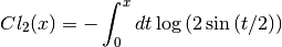
It is related to the dilogarithm by
 .
The Clausen functions are declared in the header file
.
The Clausen functions are declared in the header file
gsl_sf_clausen.h.
-
double gsl_sf_clausen(double x)
-
int gsl_sf_clausen_e(double x, gsl_sf_result *result)
These routines compute the Clausen integral
 .
.
Coulomb Functions
The prototypes of the Coulomb functions are declared in the header file
gsl_sf_coulomb.h. Both bound state and scattering solutions are
available.
Normalized Hydrogenic Bound States
-
double gsl_sf_hydrogenicR_1(double Z, double r)
-
int gsl_sf_hydrogenicR_1_e(double Z, double r, gsl_sf_result *result)
These routines compute the lowest-order normalized hydrogenic bound state radial wavefunction
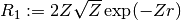 .
.
-
double gsl_sf_hydrogenicR(int n, int l, double Z, double r)
-
int gsl_sf_hydrogenicR_e(int n, int l, double Z, double r, gsl_sf_result *result)
These routines compute the
n-th normalized hydrogenic bound state radial wavefunction,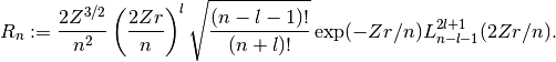
where
 is the generalized Laguerre polynomial.
The normalization is chosen such that the wavefunction
is the generalized Laguerre polynomial.
The normalization is chosen such that the wavefunction  is
given by
is
given by 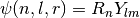 .
.
Coulomb Wave Functions
The Coulomb wave functions  ,
,  are
described in Abramowitz & Stegun, Chapter 14. Because there can be a
large dynamic range of values for these functions, overflows are handled
gracefully. If an overflow occurs,
are
described in Abramowitz & Stegun, Chapter 14. Because there can be a
large dynamic range of values for these functions, overflows are handled
gracefully. If an overflow occurs, GSL_EOVRFLW is signalled and
exponent(s) are returned through the modifiable parameters exp_F,
exp_G. The full solution can be reconstructed from the following
relations,
![F_L(\eta,x) &= fc[k_L] * \exp(exp_F) \\
G_L(\eta,x) &= gc[k_L] * \exp(exp_G)](_images/math/6190fd08dc74c14aa85c0b7c42a5d364ceb6aa30.png)
![F_L'(\eta,x) &= fcp[k_L] * \exp(exp_F) \\
G_L'(\eta,x) &= gcp[k_L] * \exp(exp_G)](_images/math/f3620d8d9a3906043a593fe219a6825784b0282a.png)
-
int gsl_sf_coulomb_wave_FG_e(double eta, double x, double L_F, int k, gsl_sf_result *F, gsl_sf_result *Fp, gsl_sf_result *G, gsl_sf_result *Gp, double *exp_F, double *exp_G)
This function computes the Coulomb wave functions
,
 and their derivatives
 ,
,
 with respect to . The parameters are restricted to
  ,
and integer
,
and integer  . Note that
  itself is not restricted to being an integer. The results are stored in
the parameters F, G for the function values and
itself is not restricted to being an integer. The results are stored in
the parameters F, G for the function values and Fp,Gpfor the derivative values. If an overflow occurs,GSL_EOVRFLWis returned and scaling exponents are stored in the modifiable parametersexp_F,exp_G.
-
int gsl_sf_coulomb_wave_F_array(double L_min, int kmax, double eta, double x, double fc_array[], double *F_exponent)
This function computes the Coulomb wave function
for
 , storing the results in
 fc_array. In the case of overflow the exponent is stored inF_exponent.
-
int gsl_sf_coulomb_wave_FG_array(double L_min, int kmax, double eta, double x, double fc_array[], double gc_array[], double *F_exponent, double *G_exponent)
This function computes the functions
,
for storing the
results in fc_arrayandgc_array. In the case of overflow the exponents are stored inF_exponentandG_exponent.
-
int gsl_sf_coulomb_wave_FGp_array(double L_min, int kmax, double eta, double x, double fc_array[], double fcp_array[], double gc_array[], double gcp_array[], double *F_exponent, double *G_exponent)
This function computes the functions
,
and their derivatives ,
 for storing the
results in
for storing the
results in fc_array,gc_array,fcp_arrayandgcp_array. In the case of overflow the exponents are stored inF_exponentandG_exponent.
-
int gsl_sf_coulomb_wave_sphF_array(double L_min, int kmax, double eta, double x, double fc_array[], double F_exponent[])
This function computes the Coulomb wave function divided by the argument
 for , storing the
results in
for , storing the
results in fc_array. In the case of overflow the exponent is stored inF_exponent. This function reduces to spherical Bessel functions in the limit .
.
Coulomb Wave Function Normalization Constant
The Coulomb wave function normalization constant is defined in Abramowitz 14.1.7.
-
int gsl_sf_coulomb_CL_e(double L, double eta, gsl_sf_result *result)
This function computes the Coulomb wave function normalization constant
 for
for  .
.
-
int gsl_sf_coulomb_CL_array(double Lmin, int kmax, double eta, double cl[])
This function computes the Coulomb wave function normalization constant
for ,  .
.
Coupling Coefficients
The Wigner 3-j, 6-j and 9-j symbols give the coupling coefficients for
combined angular momentum vectors. Since the arguments of the standard
coupling coefficient functions are integer or half-integer, the
arguments of the following functions are, by convention, integers equal
to twice the actual spin value. For information on the 3-j coefficients
see Abramowitz & Stegun, Section 27.9. The functions described in this
section are declared in the header file gsl_sf_coupling.h.
3-j Symbols
-
double gsl_sf_coupling_3j(int two_ja, int two_jb, int two_jc, int two_ma, int two_mb, int two_mc)
-
int gsl_sf_coupling_3j_e(int two_ja, int two_jb, int two_jc, int two_ma, int two_mb, int two_mc, gsl_sf_result *result)
These routines compute the Wigner 3-j coefficient,
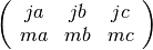
where the arguments are given in half-integer units,
 =
=
two_ja/2, =
= two_ma/2, etc.
6-j Symbols
-
double gsl_sf_coupling_6j(int two_ja, int two_jb, int two_jc, int two_jd, int two_je, int two_jf)
-
int gsl_sf_coupling_6j_e(int two_ja, int two_jb, int two_jc, int two_jd, int two_je, int two_jf, gsl_sf_result *result)
These routines compute the Wigner 6-j coefficient,
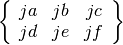
where the arguments are given in half-integer units,
=
two_ja/2, = two_ma/2, etc.
9-j Symbols
-
double gsl_sf_coupling_9j(int two_ja, int two_jb, int two_jc, int two_jd, int two_je, int two_jf, int two_jg, int two_jh, int two_ji)
-
int gsl_sf_coupling_9j_e(int two_ja, int two_jb, int two_jc, int two_jd, int two_je, int two_jf, int two_jg, int two_jh, int two_ji, gsl_sf_result *result)
These routines compute the Wigner 9-j coefficient,
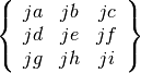
where the arguments are given in half-integer units,
=
two_ja/2, = two_ma/2, etc.
Dawson Function
The Dawson integral is defined by
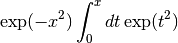
A table of Dawson’s integral can be found in Abramowitz &
Stegun, Table 7.5. The Dawson functions are declared in the header file
gsl_sf_dawson.h.
-
double gsl_sf_dawson(double x)
-
int gsl_sf_dawson_e(double x, gsl_sf_result *result)
These routines compute the value of Dawson’s integral for
x.
Debye Functions
The Debye functions  are defined by the following integral,
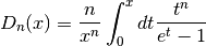
For further information see Abramowitz &
Stegun, Section 27.1. The Debye functions are declared in the header
file gsl_sf_debye.h.
-
double gsl_sf_debye_1(double x)
-
int gsl_sf_debye_1_e(double x, gsl_sf_result *result)
These routines compute the first-order Debye function
 .
.
-
double gsl_sf_debye_2(double x)
-
int gsl_sf_debye_2_e(double x, gsl_sf_result *result)
These routines compute the second-order Debye function
 .
.
-
double gsl_sf_debye_3(double x)
-
int gsl_sf_debye_3_e(double x, gsl_sf_result *result)
These routines compute the third-order Debye function
 .
.
-
double gsl_sf_debye_4(double x)
-
int gsl_sf_debye_4_e(double x, gsl_sf_result *result)
These routines compute the fourth-order Debye function
 .
.
-
double gsl_sf_debye_5(double x)
-
int gsl_sf_debye_5_e(double x, gsl_sf_result *result)
These routines compute the fifth-order Debye function
 .
.
-
double gsl_sf_debye_6(double x)
-
int gsl_sf_debye_6_e(double x, gsl_sf_result *result)
These routines compute the sixth-order Debye function
 .
.
Dilogarithm
The dilogarithm is defined as
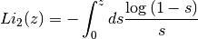
The functions described in this section are declared in the header file
gsl_sf_dilog.h.
Real Argument
-
double gsl_sf_dilog(double x)
-
int gsl_sf_dilog_e(double x, gsl_sf_result *result)
These routines compute the dilogarithm for a real argument. In Lewin’s notation this is
 , the real part of the dilogarithm of a
real . It is defined by the integral representation
, the real part of the dilogarithm of a
real . It is defined by the integral representation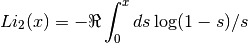
Note that
 for
for
 , and
, and  for
for  .
.Note that Abramowitz & Stegun refer to the Spence integral
 as the dilogarithm rather than .
Complex Argument
-
int gsl_sf_complex_dilog_e(double r, double theta, gsl_sf_result *result_re, gsl_sf_result *result_im)
This function computes the full complex-valued dilogarithm for the complex argument
 . The real and imaginary
parts of the result are returned in
. The real and imaginary
parts of the result are returned in result_re,result_im.
Elementary Operations
The following functions allow for the propagation of errors when
combining quantities by multiplication. The functions are declared in
the header file gsl_sf_elementary.h.
 is stored in
 Elliptic Integrals
The functions described in this section are declared in the header
file gsl_sf_ellint.h. Further information about the elliptic
integrals can be found in Abramowitz & Stegun, Chapter 17.
Definition of Legendre Forms
The Legendre forms of elliptic integrals  ,
,
 and
and  are defined by,
The complete Legendre forms are denoted by  and
and
 .
.
The notation used here is based on Carlson, “Numerische
Mathematik” 33 (1979) 1 and differs slightly from that used by
Abramowitz & Stegun, where the functions are given in terms of the
parameter  and is replaced by
  .
.
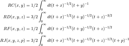
Definition of Carlson Forms
The Carlson symmetric forms of elliptical integrals  ,
,
 ,
,  and
and 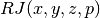 are defined
by,
are defined
by,
Legendre Form of Complete Elliptic Integrals
-
double gsl_sf_ellint_Kcomp(double k, gsl_mode_t mode)
-
int gsl_sf_ellint_Kcomp_e(double k, gsl_mode_t mode, gsl_sf_result *result)
These routines compute the complete elliptic integral
 to
the accuracy specified by the mode variable
to
the accuracy specified by the mode variable mode. Note that Abramowitz & Stegun define this function in terms of the parameter.
-
double gsl_sf_ellint_Ecomp(double k, gsl_mode_t mode)
-
int gsl_sf_ellint_Ecomp_e(double k, gsl_mode_t mode, gsl_sf_result *result)
These routines compute the complete elliptic integral
 to the
accuracy specified by the mode variable
to the
accuracy specified by the mode variable mode. Note that Abramowitz & Stegun define this function in terms of the parameter.
-
double gsl_sf_ellint_Pcomp(double k, double n, gsl_mode_t mode)
-
int gsl_sf_ellint_Pcomp_e(double k, double n, gsl_mode_t mode, gsl_sf_result *result)
These routines compute the complete elliptic integral
 to the
accuracy specified by the mode variable
to the
accuracy specified by the mode variable mode. Note that Abramowitz & Stegun define this function in terms of the parameters and  , with the
change of sign
, with the
change of sign  .
.
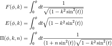
Legendre Form of Incomplete Elliptic Integrals
-
double gsl_sf_ellint_F(double phi, double k, gsl_mode_t mode)
-
int gsl_sf_ellint_F_e(double phi, double k, gsl_mode_t mode, gsl_sf_result *result)
These routines compute the incomplete elliptic integral
to the accuracy specified by the mode variable mode. Note that Abramowitz & Stegun define this function in terms of the parameter.
-
double gsl_sf_ellint_E(double phi, double k, gsl_mode_t mode)
-
int gsl_sf_ellint_E_e(double phi, double k, gsl_mode_t mode, gsl_sf_result *result)
These routines compute the incomplete elliptic integral
to the accuracy specified by the mode variable mode. Note that Abramowitz & Stegun define this function in terms of the parameter.
-
double gsl_sf_ellint_P(double phi, double k, double n, gsl_mode_t mode)
-
int gsl_sf_ellint_P_e(double phi, double k, double n, gsl_mode_t mode, gsl_sf_result *result)
These routines compute the incomplete elliptic integral
to the accuracy specified by the mode variable mode. Note that Abramowitz & Stegun define this function in terms of the parameters and , with the
change of sign .
-
double gsl_sf_ellint_D(double phi, double k, gsl_mode_t mode)
-
int gsl_sf_ellint_D_e(double phi, double k, gsl_mode_t mode, gsl_sf_result *result)
These functions compute the incomplete elliptic integral
 which is defined through the Carlson form
by the following relation,
which is defined through the Carlson form
by the following relation,
Carlson Forms
-
double gsl_sf_ellint_RC(double x, double y, gsl_mode_t mode)
-
int gsl_sf_ellint_RC_e(double x, double y, gsl_mode_t mode, gsl_sf_result *result)
These routines compute the incomplete elliptic integral
to the accuracy specified by the mode variable mode.
-
double gsl_sf_ellint_RD(double x, double y, double z, gsl_mode_t mode)
-
int gsl_sf_ellint_RD_e(double x, double y, double z, gsl_mode_t mode, gsl_sf_result *result)
These routines compute the incomplete elliptic integral
to the accuracy specified by the mode variable mode.
-
double gsl_sf_ellint_RF(double x, double y, double z, gsl_mode_t mode)
-
int gsl_sf_ellint_RF_e(double x, double y, double z, gsl_mode_t mode, gsl_sf_result *result)
These routines compute the incomplete elliptic integral
to the accuracy specified by the mode variable mode.
-
double gsl_sf_ellint_RJ(double x, double y, double z, double p, gsl_mode_t mode)
-
int gsl_sf_ellint_RJ_e(double x, double y, double z, double p, gsl_mode_t mode, gsl_sf_result *result)
These routines compute the incomplete elliptic integral
to the accuracy specified by the mode variable mode.
Elliptic Functions (Jacobi)
The Jacobian Elliptic functions are defined in Abramowitz & Stegun,
Chapter 16. The functions are declared in the header file
gsl_sf_elljac.h.
-
int gsl_sf_elljac_e(double u, double m, double *sn, double *cn, double *dn)
This function computes the Jacobian elliptic functions
 ,
,
 ,
,  by descending Landen
transformations.
by descending Landen
transformations.
Error Functions
The error function is described in Abramowitz & Stegun, Chapter 7. The
functions in this section are declared in the header file
gsl_sf_erf.h.
Error Function
-
double gsl_sf_erf(double x)
-
int gsl_sf_erf_e(double x, gsl_sf_result *result)
These routines compute the error function
 ,
where
,
where
 .
.
Complementary Error Function
-
double gsl_sf_erfc(double x)
-
int gsl_sf_erfc_e(double x, gsl_sf_result *result)
These routines compute the complementary error function

Log Complementary Error Function
-
double gsl_sf_log_erfc(double x)
-
int gsl_sf_log_erfc_e(double x, gsl_sf_result *result)
These routines compute the logarithm of the complementary error function
 .
.
Probability functions
The probability functions for the Normal or Gaussian distribution are described in Abramowitz & Stegun, Section 26.2.
-
double gsl_sf_erf_Z(double x)
-
int gsl_sf_erf_Z_e(double x, gsl_sf_result *result)
These routines compute the Gaussian probability density function

-
double gsl_sf_erf_Q(double x)
-
int gsl_sf_erf_Q_e(double x, gsl_sf_result *result)
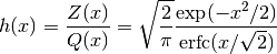
These routines compute the upper tail of the Gaussian probability function

The hazard function for the normal distribution, also known as the inverse Mills’ ratio, is defined as,
It decreases rapidly as approaches  and asymptotes
to
and asymptotes
to  as approaches
  .
.
-
double gsl_sf_hazard(double x)
-
int gsl_sf_hazard_e(double x, gsl_sf_result *result)
These routines compute the hazard function for the normal distribution.
Exponential Functions
The functions described in this section are declared in the header file
gsl_sf_exp.h.
Exponential Function
-
double gsl_sf_exp(double x)
-
int gsl_sf_exp_e(double x, gsl_sf_result *result)
These routines provide an exponential function
 using GSL
semantics and error checking.
using GSL
semantics and error checking.
-
int gsl_sf_exp_e10_e(double x, gsl_sf_result_e10 *result)
This function computes the exponential
using the
gsl_sf_result_e10type to return a result with extended range. This function may be useful if the value of would
overflow the numeric range of double.
-
double gsl_sf_exp_mult(double x, double y)
-
int gsl_sf_exp_mult_e(double x, double y, gsl_sf_result *result)
These routines exponentiate
xand multiply by the factoryto return the product .
.
-
int gsl_sf_exp_mult_e10_e(const double x, const double y, gsl_sf_result_e10 *result)
This function computes the product
using the
gsl_sf_result_e10type to return a result with extended numeric range.
Relative Exponential Functions
-
double gsl_sf_expm1(double x)
-
int gsl_sf_expm1_e(double x, gsl_sf_result *result)
These routines compute the quantity
 using an algorithm
that is accurate for small .
using an algorithm
that is accurate for small .
-
double gsl_sf_exprel(double x)
-
int gsl_sf_exprel_e(double x, gsl_sf_result *result)
These routines compute the quantity
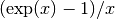 using an
algorithm that is accurate for small
using an
algorithm that is accurate for small x. For smallxthe algorithm is based on the expansion .
.
-
double gsl_sf_exprel_2(double x)
-
int gsl_sf_exprel_2_e(double x, gsl_sf_result *result)
These routines compute the quantity
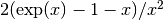 using an
algorithm that is accurate for small
using an
algorithm that is accurate for small x. For smallxthe algorithm is based on the expansion .
.
-
double gsl_sf_exprel_n(int n, double x)
-
int gsl_sf_exprel_n_e(int n, double x, gsl_sf_result *result)
These routines compute the
 -relative exponential, which is the
n-th generalization of the functionsgsl_sf_exprel()andgsl_sf_exprel_2(). The-relative exponential is given by,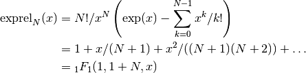
Exponentiation With Error Estimate
-
int gsl_sf_exp_err_e(double x, double dx, gsl_sf_result *result)
This function exponentiates
xwith an associated absolute errordx.
-
int gsl_sf_exp_err_e10_e(double x, double dx, gsl_sf_result_e10 *result)
This function exponentiates a quantity
xwith an associated absolute errordxusing thegsl_sf_result_e10type to return a result with extended range.
-
int gsl_sf_exp_mult_err_e(double x, double dx, double y, double dy, gsl_sf_result *result)
This routine computes the product
for the quantities
x,ywith associated absolute errorsdx,dy.
-
int gsl_sf_exp_mult_err_e10_e(double x, double dx, double y, double dy, gsl_sf_result_e10 *result)
This routine computes the product
for the quantities
x,ywith associated absolute errorsdx,dyusing thegsl_sf_result_e10type to return a result with extended range.
Exponential Integrals
Information on the exponential integrals can be found in Abramowitz &
Stegun, Chapter 5. These functions are declared in the header file
gsl_sf_expint.h.
Exponential Integral
-
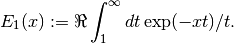
double gsl_sf_expint_E1(double x)
-
int gsl_sf_expint_E1_e(double x, gsl_sf_result *result)
These routines compute the exponential integral
 ,
,
-
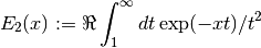
double gsl_sf_expint_E2(double x)
-
int gsl_sf_expint_E2_e(double x, gsl_sf_result *result)
These routines compute the second-order exponential integral
 ,
,
-
double gsl_sf_expint_En(int n, double x)
-
int gsl_sf_expint_En_e(int n, double x, gsl_sf_result *result)
These routines compute the exponential integral
 of order
 n,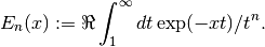
Ei(x)
-
double gsl_sf_expint_Ei(double x)
-
int gsl_sf_expint_Ei_e(double x, gsl_sf_result *result)
These routines compute the exponential integral
 ,
,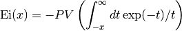
where
 denotes the principal value of the integral.
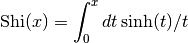
Hyperbolic Integrals
-
double gsl_sf_Shi(double x)
-
int gsl_sf_Shi_e(double x, gsl_sf_result *result)
These routines compute the integral
-
double gsl_sf_Chi(double x)
-
int gsl_sf_Chi_e(double x, gsl_sf_result *result)
These routines compute the integral
![\hbox{Chi}(x) := \Re \left[ \gamma_E + \log(x) + \int_0^x dt (\cosh(t)-1)/t \right]](_images/math/8df3dad937a6dbd0ce68a7b32ea0646a2b1153d1.png)
where
 is the Euler constant (available as the macro
 M_EULER).
Ei_3(x)
-
double gsl_sf_expint_3(double x)
-
int gsl_sf_expint_3_e(double x, gsl_sf_result *result)
These routines compute the third-order exponential integral
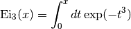
for
 .
.
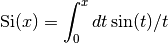
Trigonometric Integrals
-
double gsl_sf_Si(const double x)
-
int gsl_sf_Si_e(double x, gsl_sf_result *result)
These routines compute the Sine integral
-
double gsl_sf_Ci(const double x)
-
int gsl_sf_Ci_e(double x, gsl_sf_result *result)
These routines compute the Cosine integral
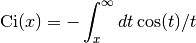
for
Arctangent Integral
-
double gsl_sf_atanint(double x)
-
int gsl_sf_atanint_e(double x, gsl_sf_result *result)
These routines compute the Arctangent integral, which is defined as
Fermi-Dirac Function
The functions described in this section are declared in the header file
gsl_sf_fermi_dirac.h.
Complete Fermi-Dirac Integrals
The complete Fermi-Dirac integral  is given by,
Note that the Fermi-Dirac integral is sometimes defined without the normalisation factor in other texts.
-
double gsl_sf_fermi_dirac_m1(double x)
-
int gsl_sf_fermi_dirac_m1_e(double x, gsl_sf_result *result)
These routines compute the complete Fermi-Dirac integral with an index of
 .
This integral is given by
.
This integral is given by
 .
.
-
double gsl_sf_fermi_dirac_0(double x)
-
int gsl_sf_fermi_dirac_0_e(double x, gsl_sf_result *result)
These routines compute the complete Fermi-Dirac integral with an index of
 .
This integral is given by
.
This integral is given by  .
.
-
double gsl_sf_fermi_dirac_1(double x)
-
int gsl_sf_fermi_dirac_1_e(double x, gsl_sf_result *result)
These routines compute the complete Fermi-Dirac integral with an index of
 ,
,
 .
.
-
double gsl_sf_fermi_dirac_2(double x)
-
int gsl_sf_fermi_dirac_2_e(double x, gsl_sf_result *result)
These routines compute the complete Fermi-Dirac integral with an index of
 ,
,
 .
.
-
double gsl_sf_fermi_dirac_int(int j, double x)
-
int gsl_sf_fermi_dirac_int_e(int j, double x, gsl_sf_result *result)
These routines compute the complete Fermi-Dirac integral with an integer index of
 ,
,
 .
.
-
double gsl_sf_fermi_dirac_mhalf(double x)
-
int gsl_sf_fermi_dirac_mhalf_e(double x, gsl_sf_result *result)
These routines compute the complete Fermi-Dirac integral
 .
.
-
double gsl_sf_fermi_dirac_half(double x)
-
int gsl_sf_fermi_dirac_half_e(double x, gsl_sf_result *result)
These routines compute the complete Fermi-Dirac integral
 .
.
-
double gsl_sf_fermi_dirac_3half(double x)
-
int gsl_sf_fermi_dirac_3half_e(double x, gsl_sf_result *result)
These routines compute the complete Fermi-Dirac integral
 .
.
Incomplete Fermi-Dirac Integrals
The incomplete Fermi-Dirac integral  is given by,
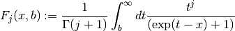
-
double gsl_sf_fermi_dirac_inc_0(double x, double b)
-
int gsl_sf_fermi_dirac_inc_0_e(double x, double b, gsl_sf_result *result)
These routines compute the incomplete Fermi-Dirac integral with an index of zero,

Gamma and Beta Functions
The following routines compute the gamma and beta functions in their
full and incomplete forms, as well as various kinds of factorials.
The functions described in this section are declared in the header
file gsl_sf_gamma.h.
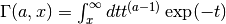
Gamma Functions
The Gamma function is defined by the following integral,
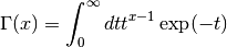
It is related to the factorial function by 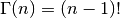 for positive integer . Further information on the Gamma function
can be found in Abramowitz & Stegun, Chapter 6.
for positive integer . Further information on the Gamma function
can be found in Abramowitz & Stegun, Chapter 6.
-
double gsl_sf_gamma(double x)
-
int gsl_sf_gamma_e(double x, gsl_sf_result *result)
These routines compute the Gamma function
 , subject to
not being a negative integer or zero. The function is computed using the real
Lanczos method. The maximum value of such that is not
considered an overflow is given by the macro
, subject to
not being a negative integer or zero. The function is computed using the real
Lanczos method. The maximum value of such that is not
considered an overflow is given by the macro GSL_SF_GAMMA_XMAXand is 171.0.
-
double gsl_sf_lngamma(double x)
-
int gsl_sf_lngamma_e(double x, gsl_sf_result *result)
These routines compute the logarithm of the Gamma function,
 , subject to not being a negative
integer or zero. For the real part of is
returned, which is equivalent to
, subject to not being a negative
integer or zero. For the real part of is
returned, which is equivalent to  . The function
is computed using the real Lanczos method.
. The function
is computed using the real Lanczos method.
-
int gsl_sf_lngamma_sgn_e(double x, gsl_sf_result *result_lg, double *sgn)
This routine computes the sign of the gamma function and the logarithm of its magnitude, subject to
not being a negative integer or zero. The
function is computed using the real Lanczos method. The value of the
gamma function and its error can be reconstructed using the relation
 , taking into account the two
components of
, taking into account the two
components of result_lg.
-
double gsl_sf_gammastar(double x)
-
int gsl_sf_gammastar_e(double x, gsl_sf_result *result)
These routines compute the regulated Gamma Function
 for . The regulated gamma function is given by,
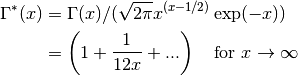
and is a useful suggestion of Temme.
-
double gsl_sf_gammainv(double x)
-
int gsl_sf_gammainv_e(double x, gsl_sf_result *result)
These routines compute the reciprocal of the gamma function,
 using the real Lanczos method.
-
int gsl_sf_lngamma_complex_e(double zr, double zi, gsl_sf_result *lnr, gsl_sf_result *arg)
This routine computes
 for complex
  and
and  not a negative integer or zero, using the complex Lanczos
method. The returned parameters are
not a negative integer or zero, using the complex Lanczos
method. The returned parameters are  and
and
 in
in ![(-\pi,\pi]](_images/math/f5aebcae7457b93a1bdbbaea798fa93f72a31d0d.png) . Note that the phase
part (
. Note that the phase
part (arg) is not well-determined when is very large,
due to inevitable roundoff in restricting to . This
will result in a
is very large,
due to inevitable roundoff in restricting to . This
will result in a GSL_ELOSSerror when it occurs. The absolute value part (lnr), however, never suffers from loss of precision.
Factorials
Although factorials can be computed from the Gamma function, using
the relation  for non-negative integer ,
it is usually more efficient to call the functions in this section,
particularly for small values of , whose factorial values are
maintained in hardcoded tables.
for non-negative integer ,
it is usually more efficient to call the functions in this section,
particularly for small values of , whose factorial values are
maintained in hardcoded tables.
-
double gsl_sf_fact(unsigned int n)
-
int gsl_sf_fact_e(unsigned int n, gsl_sf_result *result)
These routines compute the factorial
 . The factorial is
related to the Gamma function by .
The maximum value of such that is not
considered an overflow is given by the macro
. The factorial is
related to the Gamma function by .
The maximum value of such that is not
considered an overflow is given by the macro GSL_SF_FACT_NMAXand is 170.
-
double gsl_sf_doublefact(unsigned int n)
-
int gsl_sf_doublefact_e(unsigned int n, gsl_sf_result *result)
These routines compute the double factorial
 .
The maximum value of such that
.
The maximum value of such that  is not
considered an overflow is given by the macro
is not
considered an overflow is given by the macro GSL_SF_DOUBLEFACT_NMAXand is 297.
-
double gsl_sf_lnfact(unsigned int n)
-
int gsl_sf_lnfact_e(unsigned int n, gsl_sf_result *result)
These routines compute the logarithm of the factorial of
n, . The algorithm is faster than computing
 via
via gsl_sf_lngamma()for ,
but defers for larger
,
but defers for larger n.
-
double gsl_sf_lndoublefact(unsigned int n)
-
int gsl_sf_lndoublefact_e(unsigned int n, gsl_sf_result *result)
These routines compute the logarithm of the double factorial of
n, .
.
-
double gsl_sf_choose(unsigned int n, unsigned int m)
-
int gsl_sf_choose_e(unsigned int n, unsigned int m, gsl_sf_result *result)
These routines compute the combinatorial factor
n choose m
-
double gsl_sf_lnchoose(unsigned int n, unsigned int m)
-
int gsl_sf_lnchoose_e(unsigned int n, unsigned int m, gsl_sf_result *result)
These routines compute the logarithm of
n choose m. This is equivalent to the sum .
.
-
double gsl_sf_taylorcoeff(int n, double x)
-
int gsl_sf_taylorcoeff_e(int n, double x, gsl_sf_result *result)
These routines compute the Taylor coefficient
 for
,
for
, 
Pochhammer Symbol
-
double gsl_sf_poch(double a, double x)
-
int gsl_sf_poch_e(double a, double x, gsl_sf_result *result)
These routines compute the Pochhammer symbol
 .
The Pochhammer symbol is also known as the Apell symbol and
sometimes written as
.
The Pochhammer symbol is also known as the Apell symbol and
sometimes written as  . When
  and
and  are negative integers or zero, the limiting value of the ratio is returned.
-
double gsl_sf_lnpoch(double a, double x)
-
int gsl_sf_lnpoch_e(double a, double x, gsl_sf_result *result)
These routines compute the logarithm of the Pochhammer symbol,
 .
.
-
int gsl_sf_lnpoch_sgn_e(double a, double x, gsl_sf_result *result, double *sgn)
These routines compute the sign of the Pochhammer symbol and the logarithm of its magnitude. The computed parameters are
 with a corresponding error term, and
  where .
-
double gsl_sf_pochrel(double a, double x)
-
int gsl_sf_pochrel_e(double a, double x, gsl_sf_result *result)
These routines compute the relative Pochhammer symbol
 where .
Incomplete Gamma Functions
-
double gsl_sf_gamma_inc(double a, double x)
-
int gsl_sf_gamma_inc_e(double a, double x, gsl_sf_result *result)
These functions compute the unnormalized incomplete Gamma Function
 for real and .
-
double gsl_sf_gamma_inc_Q(double a, double x)
-
int gsl_sf_gamma_inc_Q_e(double a, double x, gsl_sf_result *result)
These routines compute the normalized incomplete Gamma Function
 for
for  , .
, .
-
double gsl_sf_gamma_inc_P(double a, double x)
-
int gsl_sf_gamma_inc_P_e(double a, double x, gsl_sf_result *result)
These routines compute the complementary normalized incomplete Gamma Function
 for , .
Note that Abramowitz & Stegun call
 the incomplete gamma
function (section 6.5).
the incomplete gamma
function (section 6.5).
Beta Functions
-
double gsl_sf_beta(double a, double b)
-
int gsl_sf_beta_e(double a, double b, gsl_sf_result *result)
These routines compute the Beta Function,
 subject to and
  not being negative integers.
-
double gsl_sf_lnbeta(double a, double b)
-
int gsl_sf_lnbeta_e(double a, double b, gsl_sf_result *result)
These routines compute the logarithm of the Beta Function,
 subject to and not being negative integers.
Incomplete Beta Function
-
double gsl_sf_beta_inc(double a, double b, double x)
-
int gsl_sf_beta_inc_e(double a, double b, double x, gsl_sf_result *result)
These routines compute the normalized incomplete Beta function
 where
where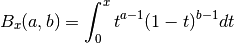
for
 .
For ,
.
For ,  the value is computed using
a continued fraction expansion. For all other values it is computed using
the relation
the value is computed using
a continued fraction expansion. For all other values it is computed using
the relation
Gegenbauer Functions
The Gegenbauer polynomials are defined in Abramowitz & Stegun, Chapter
22, where they are known as Ultraspherical polynomials. The functions
described in this section are declared in the header file
gsl_sf_gegenbauer.h.
-
double gsl_sf_gegenpoly_1(double lambda, double x)
-
double gsl_sf_gegenpoly_2(double lambda, double x)
-
double gsl_sf_gegenpoly_3(double lambda, double x)
-
int gsl_sf_gegenpoly_1_e(double lambda, double x, gsl_sf_result *result)
-
int gsl_sf_gegenpoly_2_e(double lambda, double x, gsl_sf_result *result)
-
int gsl_sf_gegenpoly_3_e(double lambda, double x, gsl_sf_result *result)
These functions evaluate the Gegenbauer polynomials
 using explicit
representations for
using explicit
representations for  .
.
-
double gsl_sf_gegenpoly_n(int n, double lambda, double x)
-
int gsl_sf_gegenpoly_n_e(int n, double lambda, double x, gsl_sf_result *result)
These functions evaluate the Gegenbauer polynomial
for a specific value of n,lambda,xsubject to , .
, .
-
int gsl_sf_gegenpoly_array(int nmax, double lambda, double x, double result_array[])
This function computes an array of Gegenbauer polynomials
for  , subject
to ,
, subject
to ,  .
.
Hermite Polynomials and Functions
Hermite polynomials and functions are discussed in Abramowitz & Stegun, Chapter 22 and
Szego, Gabor (1939, 1958, 1967), Orthogonal Polynomials, American Mathematical Society.
The Hermite polynomials and functions are defined in the header file gsl_sf_hermite.h.
Hermite Polynomials
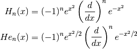
The Hermite polynomials exist in two variants: the physicist version
 and the probabilist version
  .
They are defined by the derivatives
.
They are defined by the derivatives
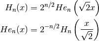
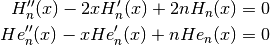
They are connected via
and satisfy the ordinary differential equations
-
double gsl_sf_hermite(const int n, const double x)
-
int gsl_sf_hermite_e(const int n, const double x, gsl_sf_result *result)
These routines evaluate the physicist Hermite polynomial
of order nat positionx. If an overflow is detected,GSL_EOVRFLWis returned without calling the error handler.
-
int gsl_sf_hermite_array(const int nmax, const double x, double *result_array)
This routine evaluates all physicist Hermite polynomials
 up to order
 nmaxat positionx. The results are stored inresult_array.
-
double gsl_sf_hermite_series(const int n, const double x, const double *a)
-
int gsl_sf_hermite_series_e(const int n, const double x, const double *a, gsl_sf_result *result)
These routines evaluate the series
 with
with  being
the -th physicist Hermite polynomial using the Clenshaw algorithm.
being
the -th physicist Hermite polynomial using the Clenshaw algorithm.
-
double gsl_sf_hermite_prob(const int n, const double x)
-
int gsl_sf_hermite_prob_e(const int n, const double x, gsl_sf_result *result)
These routines evaluate the probabilist Hermite polynomial
of order nat positionx. If an overflow is detected,GSL_EOVRFLWis returned without calling the error handler.
-
int gsl_sf_hermite_prob_array(const int nmax, const double x, double *result_array)
This routine evaluates all probabilist Hermite polynomials
up to order nmaxat positionx. The results are stored inresult_array.
-
double gsl_sf_hermite_prob_series(const int n, const double x, const double *a)
-
int gsl_sf_hermite_prob_series_e(const int n, const double x, const double *a, gsl_sf_result *result)
These routines evaluate the series
 with
with  being the
-th probabilist Hermite polynomial using the Clenshaw algorithm.
being the
-th probabilist Hermite polynomial using the Clenshaw algorithm.
Derivatives of Hermite Polynomials
-
double gsl_sf_hermite_deriv(const int m, const int n, const double x)
-
int gsl_sf_hermite_deriv_e(const int m, const int n, const double x, gsl_sf_result *result)
These routines evaluate the
m-th derivative of the physicist Hermite polynomial of order nat positionx.
-
int gsl_sf_hermite_array_deriv(const int m, const int nmax, const double x, double *result_array)
This routine evaluates the
m-th derivative of all physicist Hermite polynomials from
orders  at position
 x. The result is stored in
 result_array[n]. The outputresult_arraymust have length at leastnmax + 1.
-
int gsl_sf_hermite_deriv_array(const int mmax, const int n, const double x, double *result_array)
This routine evaluates all derivative orders from
 of the
physicist Hermite polynomial of order
of the
physicist Hermite polynomial of order n,, at position x. The result is stored in result_array[m]. The outputresult_arraymust have length at leastmmax + 1.
-
double gsl_sf_hermite_prob_deriv(const int m, const int n, const double x)
-
int gsl_sf_hermite_prob_deriv_e(const int m, const int n, const double x, gsl_sf_result *result)
These routines evaluate the
m-th derivative of the probabilist Hermite polynomial
of order nat positionx.
-
int gsl_sf_hermite_prob_array_deriv(const int m, const int nmax, const double x, double *result_array)
This routine evaluates the
m-th derivative of all probabilist Hermite polynomials from
orders at position x. The result is stored in
 result_array[n]. The outputresult_arraymust have length at leastnmax + 1.
-
int gsl_sf_hermite_prob_deriv_array(const int mmax, const int n, const double x, double *result_array)
This routine evaluates all derivative orders from
of the
probabilist Hermite polynomial of order n, , at position
 x. The result is stored in result_array[m]. The outputresult_arraymust have length at leastmmax + 1.
Hermite Functions
The Hermite functions are defined by
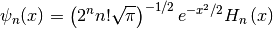
and satisfy the Schrödinger equation for a quantum mechanical harmonic oscillator

They are orthonormal,
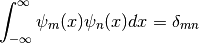
and form an orthonormal basis of  . The Hermite functions
are also eigenfunctions of the continuous Fourier transform. GSL offers two
methods for evaluating the Hermite functions. The first uses the standard three-term
recurrence relation which has
. The Hermite functions
are also eigenfunctions of the continuous Fourier transform. GSL offers two
methods for evaluating the Hermite functions. The first uses the standard three-term
recurrence relation which has  complexity and is the most accurate. The
second uses a Cauchy integral approach due to Bunck (2009) which has
complexity and is the most accurate. The
second uses a Cauchy integral approach due to Bunck (2009) which has  complexity which represents a significant speed improvement for large , although
it is slightly less accurate.
complexity which represents a significant speed improvement for large , although
it is slightly less accurate.
-
double gsl_sf_hermite_func(const int n, const double x)
-
int gsl_sf_hermite_func_e(const int n, const double x, gsl_sf_result *result)
These routines evaluate the Hermite function
 of order
 nat positionxusing a three term recurrence relation. The algorithm complexity is.
-
double gsl_sf_hermite_func_fast(const int n, const double x)
-
int gsl_sf_hermite_func_fast_e(const int n, const double x, gsl_sf_result *result)
These routines evaluate the Hermite function
of order nat positionxusing a the Cauchy integral algorithm due to Bunck, 2009. The algorithm complexity is.
-
int gsl_sf_hermite_func_array(const int nmax, const double x, double *result_array)
This routine evaluates all Hermite functions
for orders  at position
 x, using the recurrence relation algorithm. The results are stored inresult_arraywhich has length at leastnmax + 1.
-
double gsl_sf_hermite_func_series(const int n, const double x, const double *a)
-
int gsl_sf_hermite_func_series_e(const int n, const double x, const double *a, gsl_sf_result *result)
These routines evaluate the series
 with
with  being
the -th Hermite function using the Clenshaw algorithm.
being
the -th Hermite function using the Clenshaw algorithm.
Derivatives of Hermite Functions
Zeros of Hermite Polynomials and Hermite Functions
These routines calculate the  -th zero of the Hermite polynomial/function of order
. Since the zeros are symmetrical around zero, only positive zeros are calculated,
ordered from smallest to largest, starting from index 1. Only for odd polynomial orders a
zeroth zero exists, its value always being zero.
-th zero of the Hermite polynomial/function of order
. Since the zeros are symmetrical around zero, only positive zeros are calculated,
ordered from smallest to largest, starting from index 1. Only for odd polynomial orders a
zeroth zero exists, its value always being zero.
-
double gsl_sf_hermite_zero(const int n, const int s)
-
int gsl_sf_hermite_zero_e(const int n, const int s, gsl_sf_result *result)
These routines evaluate the
s-th zero of the physicist Hermite polynomial of order n.
-
double gsl_sf_hermite_prob_zero(const int n, const int s)
-
int gsl_sf_hermite_prob_zero_e(const int n, const int s, gsl_sf_result *result)
These routines evaluate the
s-th zero of the probabilist Hermite polynomial of order n.
-
double gsl_sf_hermite_func_zero(const int n, const int s)
-
int gsl_sf_hermite_func_zero_e(const int n, const int s, gsl_sf_result *result)
These routines evaluate the
s-th zero of the Hermite function of order n.
Hypergeometric Functions
Hypergeometric functions are described in Abramowitz & Stegun, Chapters
13 and 15. These functions are declared in the header file
gsl_sf_hyperg.h.
-
double gsl_sf_hyperg_0F1(double c, double x)
-
int gsl_sf_hyperg_0F1_e(double c, double x, gsl_sf_result *result)
These routines compute the hypergeometric function

-
double gsl_sf_hyperg_1F1_int(int m, int n, double x)
-
int gsl_sf_hyperg_1F1_int_e(int m, int n, double x, gsl_sf_result *result)
These routines compute the confluent hypergeometric function

-
double gsl_sf_hyperg_1F1(double a, double b, double x)
-
int gsl_sf_hyperg_1F1_e(double a, double b, double x, gsl_sf_result *result)
These routines compute the confluent hypergeometric function

-
double gsl_sf_hyperg_U_int(int m, int n, double x)
-
int gsl_sf_hyperg_U_int_e(int m, int n, double x, gsl_sf_result *result)
These routines compute the confluent hypergeometric function
 for integer parameters
 m,n.
-
int gsl_sf_hyperg_U_int_e10_e(int m, int n, double x, gsl_sf_result_e10 *result)
This routine computes the confluent hypergeometric function
for integer parameters m,nusing thegsl_sf_result_e10type to return a result with extended range.
-
double gsl_sf_hyperg_U(double a, double b, double x)
-
int gsl_sf_hyperg_U_e(double a, double b, double x, gsl_sf_result *result)
These routines compute the confluent hypergeometric function
 .
.
-
int gsl_sf_hyperg_U_e10_e(double a, double b, double x, gsl_sf_result_e10 *result)
This routine computes the confluent hypergeometric function
using the gsl_sf_result_e10type to return a result with extended range.
-
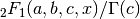
double gsl_sf_hyperg_2F1(double a, double b, double c, double x)
-
int gsl_sf_hyperg_2F1_e(double a, double b, double c, double x, gsl_sf_result *result)
These routines compute the Gauss hypergeometric function

for
 . If the arguments
  are too close to a singularity then
the function can return the error code
are too close to a singularity then
the function can return the error code GSL_EMAXITERwhen the series approximation converges too slowly. This occurs in the region of ,
,  for integer m.
-
double gsl_sf_hyperg_2F1_conj(double aR, double aI, double c, double x)
-
int gsl_sf_hyperg_2F1_conj_e(double aR, double aI, double c, double x, gsl_sf_result *result)
These routines compute the Gauss hypergeometric function

with complex parameters for
.
-
double gsl_sf_hyperg_2F1_renorm(double a, double b, double c, double x)
-
int gsl_sf_hyperg_2F1_renorm_e(double a, double b, double c, double x, gsl_sf_result *result)
These routines compute the renormalized Gauss hypergeometric function
for
.
-
double gsl_sf_hyperg_2F1_conj_renorm(double aR, double aI, double c, double x)
-
int gsl_sf_hyperg_2F1_conj_renorm_e(double aR, double aI, double c, double x, gsl_sf_result *result)
These routines compute the renormalized Gauss hypergeometric function

for
.
-
double gsl_sf_hyperg_2F0(double a, double b, double x)
-
int gsl_sf_hyperg_2F0_e(double a, double b, double x, gsl_sf_result *result)
These routines compute the hypergeometric function

The series representation is a divergent hypergeometric series. However, for
we have
Laguerre Functions
The generalized Laguerre polynomials, sometimes referred to as associated Laguerre polynomials, are defined in terms of confluent hypergeometric functions as
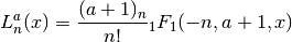
where  is the Pochhammer symbol (rising factorial).
They are related to the plain
Laguerre polynomials
is the Pochhammer symbol (rising factorial).
They are related to the plain
Laguerre polynomials  by
by  and
and
 For more information see Abramowitz & Stegun, Chapter 22.
The functions described in this section are
declared in the header file gsl_sf_laguerre.h.
-
double gsl_sf_laguerre_1(double a, double x)
-
double gsl_sf_laguerre_2(double a, double x)
-
double gsl_sf_laguerre_3(double a, double x)
-
int gsl_sf_laguerre_1_e(double a, double x, gsl_sf_result *result)
-
int gsl_sf_laguerre_2_e(double a, double x, gsl_sf_result *result)
-
int gsl_sf_laguerre_3_e(double a, double x, gsl_sf_result *result)
These routines evaluate the generalized Laguerre polynomials
 ,
,  ,
,  using explicit
representations.
using explicit
representations.
-
double gsl_sf_laguerre_n(const int n, const double a, const double x)
-
int gsl_sf_laguerre_n_e(int n, double a, double x, gsl_sf_result *result)
These routines evaluate the generalized Laguerre polynomials
 for
for  ,
.
,
.
Lambert W Functions
Lambert’s W functions,  , are defined to be solutions
of the equation
, are defined to be solutions
of the equation  . This function has
multiple branches for ; however, it has only
two real-valued branches. We define
. This function has
multiple branches for ; however, it has only
two real-valued branches. We define  to be the
principal branch, where
to be the
principal branch, where  for , and
 to be the other real branch, where
 for . The Lambert functions are
declared in the header file
for . The Lambert functions are
declared in the header file gsl_sf_lambert.h.
-
double gsl_sf_lambert_W0(double x)
-
int gsl_sf_lambert_W0_e(double x, gsl_sf_result *result)
These compute the principal branch of the Lambert W function,
.
-
double gsl_sf_lambert_Wm1(double x)
-
int gsl_sf_lambert_Wm1_e(double x, gsl_sf_result *result)
These compute the secondary real-valued branch of the Lambert W function,
.
Legendre Functions and Spherical Harmonics
The Legendre Functions and Legendre Polynomials are described in
Abramowitz & Stegun, Chapter 8. These functions are declared in
the header file gsl_sf_legendre.h.
Legendre Polynomials
-
double gsl_sf_legendre_P1(double x)
-
double gsl_sf_legendre_P2(double x)
-
double gsl_sf_legendre_P3(double x)
-
int gsl_sf_legendre_P1_e(double x, gsl_sf_result *result)
-
int gsl_sf_legendre_P2_e(double x, gsl_sf_result *result)
-
int gsl_sf_legendre_P3_e(double x, gsl_sf_result *result)
These functions evaluate the Legendre polynomials
 using explicit representations for
  .
.
-
double gsl_sf_legendre_Pl(int l, double x)
-
int gsl_sf_legendre_Pl_e(int l, double x, gsl_sf_result *result)
These functions evaluate the Legendre polynomial
for a specific value of l,xsubject to and
and
 .
.
-
int gsl_sf_legendre_Pl_array(int lmax, double x, double result_array[])
-
int gsl_sf_legendre_Pl_deriv_array(int lmax, double x, double result_array[], double result_deriv_array[])
These functions compute arrays of Legendre polynomials
and derivatives  for
for  and .
and .
-
double gsl_sf_legendre_Q0(double x)
-
int gsl_sf_legendre_Q0_e(double x, gsl_sf_result *result)
These routines compute the Legendre function
 for
for
 and
and  .
.
-
double gsl_sf_legendre_Q1(double x)
-
int gsl_sf_legendre_Q1_e(double x, gsl_sf_result *result)
These routines compute the Legendre function
 for
and .
for
and .
-
double gsl_sf_legendre_Ql(int l, double x)
-
int gsl_sf_legendre_Ql_e(int l, double x, gsl_sf_result *result)
These routines compute the Legendre function
 for
, and .
for
, and .
Associated Legendre Polynomials and Spherical Harmonics
The following functions compute the associated Legendre polynomials
 which are solutions of the differential equation

where the degree and order  satisfy
  and
and
 .
The functions grow combinatorially with
and can overflow for larger than about 150.
Alternatively, one may calculate normalized associated Legendre
polynomials. There are a number of different normalization conventions,
and these
functions can be stably computed up to degree and order 2700. The
following normalizations are provided:
.
The functions grow combinatorially with
and can overflow for larger than about 150.
Alternatively, one may calculate normalized associated Legendre
polynomials. There are a number of different normalization conventions,
and these
functions can be stably computed up to degree and order 2700. The
following normalizations are provided:
Schmidt semi-normalization
Schmidt semi-normalized associated Legendre polynomials are often used in the magnetics community and are defined as
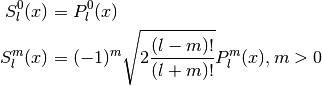
The factor of
 is called the Condon-Shortley phase
factor and can be excluded if desired by setting the parameter
is called the Condon-Shortley phase
factor and can be excluded if desired by setting the parameter
csphase = 1in the functions below.Spherical Harmonic Normalization
The associated Legendre polynomials suitable for calculating spherical harmonics are defined as
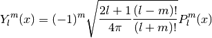
where again the phase factor
can be included or excluded
if desired.Full Normalization
The fully normalized associated Legendre polynomials are defined as
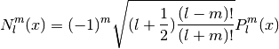
and have the property
The normalized associated Legendre routines below use a recurrence
relation which is stable up to a degree and order of about 2700.
Beyond this, the computed functions could suffer from underflow
leading to incorrect results. Routines are provided to compute
first and second derivatives
 and
and  as well as their alternate
versions
as well as their alternate
versions  and
and
 . While there is a simple
scaling relationship between the two forms, the derivatives
involving
. While there is a simple
scaling relationship between the two forms, the derivatives
involving  are heavily used in spherical harmonic
expansions and so these routines are also provided.
are heavily used in spherical harmonic
expansions and so these routines are also provided.
In the functions below, a parameter of type gsl_sf_legendre_t
specifies the type of normalization to use. The possible values are
-
type gsl_sf_legendre_t
Value
Description
GSL_SF_LEGENDRE_NONEThe unnormalized associated Legendre polynomials
GSL_SF_LEGENDRE_SCHMIDTThe Schmidt semi-normalized associated Legendre polynomials

GSL_SF_LEGENDRE_SPHARMThe spherical harmonic associated Legendre polynomials

GSL_SF_LEGENDRE_FULLThe fully normalized associated Legendre polynomials

-
int gsl_sf_legendre_array(const gsl_sf_legendre_t norm, const size_t lmax, const double x, double result_array[])
-
int gsl_sf_legendre_array_e(const gsl_sf_legendre_t norm, const size_t lmax, const double x, const double csphase, double result_array[])
These functions calculate all normalized associated Legendre polynomials for
 and
for .
The
and
for .
The normparameter specifies which normalization is used. The normalized values are stored in result_array, whose minimum size can be obtained from callinggsl_sf_legendre_array_n(). The array index of is obtained from calling
gsl_sf_legendre_array_index(l, m). To include or exclude the Condon-Shortley phase factor of, set the parameter
csphaseto either or respectively in the
_efunction. This factor is excluded by default.
-
int gsl_sf_legendre_deriv_array(const gsl_sf_legendre_t norm, const size_t lmax, const double x, double result_array[], double result_deriv_array[])
-
int gsl_sf_legendre_deriv_array_e(const gsl_sf_legendre_t norm, const size_t lmax, const double x, const double csphase, double result_array[], double result_deriv_array[])
These functions calculate all normalized associated Legendre functions and their first derivatives up to degree
lmaxfor.
The parameter normspecifies the normalization used. The normalized values and their derivatives
are stored in result_arrayandresult_deriv_arrayrespectively. To include or exclude the Condon-Shortley phase factor of, set the parameter
csphaseto either or respectively in the
_efunction. This factor is excluded by default.
-
int gsl_sf_legendre_deriv_alt_array(const gsl_sf_legendre_t norm, const size_t lmax, const double x, double result_array[], double result_deriv_array[])
-
int gsl_sf_legendre_deriv_alt_array_e(const gsl_sf_legendre_t norm, const size_t lmax, const double x, const double csphase, double result_array[], double result_deriv_array[])
These functions calculate all normalized associated Legendre functions and their (alternate) first derivatives up to degree
lmaxfor.
The normalized values and their derivatives
 are stored in
 result_arrayandresult_deriv_arrayrespectively. To include or exclude the Condon-Shortley phase factor of, set the parameter
csphaseto either or respectively in the
_efunction. This factor is excluded by default.
-
int gsl_sf_legendre_deriv2_array(const gsl_sf_legendre_t norm, const size_t lmax, const double x, double result_array[], double result_deriv_array[], double result_deriv2_array[])
-
int gsl_sf_legendre_deriv2_array_e(const gsl_sf_legendre_t norm, const size_t lmax, const double x, const double csphase, double result_array[], double result_deriv_array[], double result_deriv2_array[])
These functions calculate all normalized associated Legendre functions and their first and second derivatives up to degree
lmaxfor.
The parameter normspecifies the normalization used. The normalized, their first derivatives
, and their second derivatives
are stored in result_array,result_deriv_array, andresult_deriv2_arrayrespectively. To include or exclude the Condon-Shortley phase factor of, set the parameter
csphaseto either or respectively in the
_efunction. This factor is excluded by default.
-
int gsl_sf_legendre_deriv2_alt_array(const gsl_sf_legendre_t norm, const size_t lmax, const double x, double result_array[], double result_deriv_array[], double result_deriv2_array[])
-
int gsl_sf_legendre_deriv2_alt_array_e(const gsl_sf_legendre_t norm, const size_t lmax, const double x, const double csphase, double result_array[], double result_deriv_array[], double result_deriv2_array[])
These functions calculate all normalized associated Legendre functions and their (alternate) first and second derivatives up to degree
lmaxfor.
The parameter normspecifies the normalization used. The normalized, their first derivatives
, and their second derivatives
are stored in result_array,result_deriv_array, andresult_deriv2_arrayrespectively. To include or exclude the Condon-Shortley phase factor of, set the parameter
csphaseto either or respectively in the
_efunction. This factor is excluded by default.
-
size_t gsl_sf_legendre_nlm(const size_t lmax)
This function returns the total number of associated Legendre functions
for a given lmax. The number is(lmax+1) * (lmax+2) / 2.
-
size_t gsl_sf_legendre_array_n(const size_t lmax)
This function returns the minimum array size for maximum degree
lmaxneeded for the array versions of the associated Legendre functions. Size is calculated as the total number of functions
(see gsl_sf_legendre_nlm()), plus extra space for precomputing multiplicative factors used in the recurrence relations.
-
size_t gsl_sf_legendre_array_index(const size_t l, const size_t m)
This function returns the index into
result_array,result_deriv_array, orresult_deriv2_arraycorresponding to,  , or
, or  . The
index is given by
. The
index is given by  .
.An inline version of this function is used if
HAVE_INLINEis defined.
-
double gsl_sf_legendre_Plm(int l, int m, double x)
-
int gsl_sf_legendre_Plm_e(int l, int m, double x, gsl_sf_result *result)
These routines compute the associated Legendre polynomial
for  ,
,
 , and .
-
double gsl_sf_legendre_sphPlm(int l, int m, double x)
-
int gsl_sf_legendre_sphPlm_e(int l, int m, double x, gsl_sf_result *result)
These routines compute the normalized associated Legendre polynomial
 suitable
for use in spherical harmonics. The parameters must satisfy ,
, and .
These routines avoid the overflows
that occur for the standard normalization of .
suitable
for use in spherical harmonics. The parameters must satisfy ,
, and .
These routines avoid the overflows
that occur for the standard normalization of .
-
int gsl_sf_legendre_Plm_array(int lmax, int m, double x, double result_array[])
-
int gsl_sf_legendre_Plm_deriv_array(int lmax, int m, double x, double result_array[], double result_deriv_array[])
These functions are now deprecated and will be removed in a future release; see
gsl_sf_legendre_array()andgsl_sf_legendre_deriv_array().
-
int gsl_sf_legendre_sphPlm_array(int lmax, int m, double x, double result_array[])
-
int gsl_sf_legendre_sphPlm_deriv_array(int lmax, int m, double x, double result_array[], double result_deriv_array[])
These functions are now deprecated and will be removed in a future release; see
gsl_sf_legendre_array()andgsl_sf_legendre_deriv_array().
-
int gsl_sf_legendre_array_size(const int lmax, const int m)
This function is now deprecated and will be removed in a future release.
Conical Functions
The Conical Functions  and
and  are described in Abramowitz & Stegun, Section 8.12.
-
double gsl_sf_conicalP_half(double lambda, double x)
-
int gsl_sf_conicalP_half_e(double lambda, double x, gsl_sf_result *result)
These routines compute the irregular Spherical Conical Function
 for .
for .
-
double gsl_sf_conicalP_mhalf(double lambda, double x)
-
int gsl_sf_conicalP_mhalf_e(double lambda, double x, gsl_sf_result *result)
These routines compute the regular Spherical Conical Function
 for .
for .
-
double gsl_sf_conicalP_0(double lambda, double x)
-
int gsl_sf_conicalP_0_e(double lambda, double x, gsl_sf_result *result)
These routines compute the conical function
 for .
for .
-
double gsl_sf_conicalP_1(double lambda, double x)
-
int gsl_sf_conicalP_1_e(double lambda, double x, gsl_sf_result *result)
These routines compute the conical function
 for .
for .
-
double gsl_sf_conicalP_sph_reg(int l, double lambda, double x)
-
int gsl_sf_conicalP_sph_reg_e(int l, double lambda, double x, gsl_sf_result *result)
These routines compute the Regular Spherical Conical Function
 for and
  .
.
-
double gsl_sf_conicalP_cyl_reg(int m, double lambda, double x)
-
int gsl_sf_conicalP_cyl_reg_e(int m, double lambda, double x, gsl_sf_result *result)
These routines compute the Regular Cylindrical Conical Function
 for and
  .
.
Radial Functions for Hyperbolic Space
The following spherical functions are specializations of Legendre
functions which give the regular eigenfunctions of the Laplacian on a
3-dimensional hyperbolic space  . Of particular interest is
the flat limit,
. Of particular interest is
the flat limit,  , ,
, ,
 fixed.
-
double gsl_sf_legendre_H3d_0(double lambda, double eta)
-
int gsl_sf_legendre_H3d_0_e(double lambda, double eta, gsl_sf_result *result)
These routines compute the zeroth radial eigenfunction of the Laplacian on the 3-dimensional hyperbolic space,
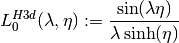
for
 .
In the flat limit this takes the form
.
In the flat limit this takes the form
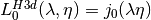 .
.
-
double gsl_sf_legendre_H3d_1(double lambda, double eta)
-
int gsl_sf_legendre_H3d_1_e(double lambda, double eta, gsl_sf_result *result)
These routines compute the first radial eigenfunction of the Laplacian on the 3-dimensional hyperbolic space,
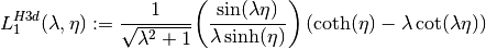
for
In the flat limit this takes the form
 .
.
-
double gsl_sf_legendre_H3d(int l, double lambda, double eta)
-
int gsl_sf_legendre_H3d_e(int l, double lambda, double eta, gsl_sf_result *result)
These routines compute the
l-th radial eigenfunction of the Laplacian on the 3-dimensional hyperbolic space and
.
In the flat limit this takes the form
 .
.
-
int gsl_sf_legendre_H3d_array(int lmax, double lambda, double eta, double result_array[])
This function computes an array of radial eigenfunctions
 for .
for .
Logarithm and Related Functions
Information on the properties of the Logarithm function can be found in
Abramowitz & Stegun, Chapter 4. The functions described in this section
are declared in the header file gsl_sf_log.h.
-
double gsl_sf_log(double x)
-
int gsl_sf_log_e(double x, gsl_sf_result *result)
These routines compute the logarithm of
x, , for
.
, for
.
-
double gsl_sf_log_abs(double x)
-
int gsl_sf_log_abs_e(double x, gsl_sf_result *result)
These routines compute the logarithm of the magnitude of
x, , for
, for  .
.
-
int gsl_sf_complex_log_e(double zr, double zi, gsl_sf_result *lnr, gsl_sf_result *theta)
This routine computes the complex logarithm of
.
The results are returned as lnr,thetasuch that , where lies in
the range
, where lies in
the range ![[-\pi,\pi]](_images/math/58bf004f12f914a4398f6b9638ee5cc7cf724392.png) .
.
-
double gsl_sf_log_1plusx(double x)
-
int gsl_sf_log_1plusx_e(double x, gsl_sf_result *result)
These routines compute
 for using an
algorithm that is accurate for small
for using an
algorithm that is accurate for small x.
-
double gsl_sf_log_1plusx_mx(double x)
-
int gsl_sf_log_1plusx_mx_e(double x, gsl_sf_result *result)
These routines compute
 for using an
algorithm that is accurate for small
for using an
algorithm that is accurate for small x.
Mathieu Functions
The routines described in this section compute the angular and radial Mathieu functions, and their characteristic values. Mathieu functions are the solutions of the following two differential equations:
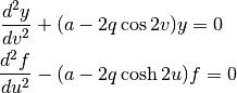
The angular Mathieu functions  ,
,  are
the even and odd periodic solutions of the first equation, which is known as Mathieu’s equation. These exist
only for the discrete sequence of characteristic values
are
the even and odd periodic solutions of the first equation, which is known as Mathieu’s equation. These exist
only for the discrete sequence of characteristic values  (even-periodic) and
  (odd-periodic).
The radial Mathieu functions  and
and
 are the solutions of the second equation,
which is referred to as Mathieu’s modified equation. The
radial Mathieu functions of the first, second, third and fourth kind
are denoted by the parameter , which takes the value 1, 2, 3
or 4.
are the solutions of the second equation,
which is referred to as Mathieu’s modified equation. The
radial Mathieu functions of the first, second, third and fourth kind
are denoted by the parameter , which takes the value 1, 2, 3
or 4.
For more information on the Mathieu functions, see Abramowitz and
Stegun, Chapter 20. These functions are defined in the header file
gsl_sf_mathieu.h.
Mathieu Function Workspace
The Mathieu functions can be computed for a single order or for multiple orders, using array-based routines. The array-based routines require a preallocated workspace.
-
type gsl_sf_mathieu_workspace
Workspace required for array-based routines
-
gsl_sf_mathieu_workspace *gsl_sf_mathieu_alloc(size_t n, double qmax)
This function returns a workspace for the array versions of the Mathieu routines. The arguments n and
qmaxspecify the maximum order and -value of Mathieu functions which can be
computed with this workspace.
-value of Mathieu functions which can be
computed with this workspace.
-
void gsl_sf_mathieu_free(gsl_sf_mathieu_workspace *work)
This function frees the workspace
work.
Mathieu Function Characteristic Values
-
int gsl_sf_mathieu_a(int n, double q)
-
int gsl_sf_mathieu_a_e(int n, double q, gsl_sf_result *result)
-
int gsl_sf_mathieu_b(int n, double q)
-
int gsl_sf_mathieu_b_e(int n, double q, gsl_sf_result *result)
These routines compute the characteristic values
 ,
,
 of the Mathieu functions
  and
and
 , respectively.
-
int gsl_sf_mathieu_a_array(int order_min, int order_max, double q, gsl_sf_mathieu_workspace *work, double result_array[])
-
int gsl_sf_mathieu_b_array(int order_min, int order_max, double q, gsl_sf_mathieu_workspace *work, double result_array[])
These routines compute a series of Mathieu characteristic values
, for from order_mintoorder_maxinclusive, storing the results in the arrayresult_array.
Angular Mathieu Functions
-
int gsl_sf_mathieu_ce(int n, double q, double x)
-
int gsl_sf_mathieu_ce_e(int n, double q, double x, gsl_sf_result *result)
-
int gsl_sf_mathieu_se(int n, double q, double x)
-
int gsl_sf_mathieu_se_e(int n, double q, double x, gsl_sf_result *result)
These routines compute the angular Mathieu functions
and , respectively.
-
int gsl_sf_mathieu_ce_array(int nmin, int nmax, double q, double x, gsl_sf_mathieu_workspace *work, double result_array[])
-
int gsl_sf_mathieu_se_array(int nmin, int nmax, double q, double x, gsl_sf_mathieu_workspace *work, double result_array[])
These routines compute a series of the angular Mathieu functions
and of order from
nmintonmaxinclusive, storing the results in the arrayresult_array.
Radial Mathieu Functions
-
int gsl_sf_mathieu_Mc(int j, int n, double q, double x)
-
int gsl_sf_mathieu_Mc_e(int j, int n, double q, double x, gsl_sf_result *result)
-
int gsl_sf_mathieu_Ms(int j, int n, double q, double x)
-
int gsl_sf_mathieu_Ms_e(int j, int n, double q, double x, gsl_sf_result *result)
These routines compute the radial
j-th kind Mathieu functions and
and  of order
 n.The allowed values of
jare 1 and 2. The functions for can be computed as
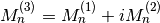 and
and
 ,
where
,
where
 or
or
 .
.
-
int gsl_sf_mathieu_Mc_array(int j, int nmin, int nmax, double q, double x, gsl_sf_mathieu_workspace *work, double result_array[])
-
int gsl_sf_mathieu_Ms_array(int j, int nmin, int nmax, double q, double x, gsl_sf_mathieu_workspace *work, double result_array[])
These routines compute a series of the radial Mathieu functions of kind
j, with order fromnmintonmaxinclusive, storing the results in the arrayresult_array.
Power Function
The following functions are equivalent to the function gsl_pow_int()
with an error estimate. These functions are
declared in the header file gsl_sf_pow_int.h.
-
double gsl_sf_pow_int(double x, int n)
-
int gsl_sf_pow_int_e(double x, int n, gsl_sf_result *result)
These routines compute the power
 for integer
 n. The power is computed using the minimum number of multiplications. For example, is computed as
  , requiring only 3
multiplications. For reasons of efficiency, these functions do not
check for overflow or underflow conditions. The following is a simple example:
, requiring only 3
multiplications. For reasons of efficiency, these functions do not
check for overflow or underflow conditions. The following is a simple example:#include <gsl/gsl_sf_pow_int.h> /* compute 3.0**12 */ double y = gsl_sf_pow_int(3.0, 12);
Psi (Digamma) Function
The polygamma functions of order are defined by
where  is known as the digamma function.
These functions are declared in the header file
is known as the digamma function.
These functions are declared in the header file gsl_sf_psi.h.
Digamma Function
-
double gsl_sf_psi_int(int n)
-
int gsl_sf_psi_int_e(int n, gsl_sf_result *result)
These routines compute the digamma function
 for positive
integer
for positive
integer n. The digamma function is also called the Psi function.
-
double gsl_sf_psi(double x)
-
int gsl_sf_psi_e(double x, gsl_sf_result *result)
These routines compute the digamma function
 for general
x,.
-
double gsl_sf_psi_1piy(double y)
-
int gsl_sf_psi_1piy_e(double y, gsl_sf_result *result)
These routines compute the real part of the digamma function on the line
 ,
, ![\Re[\psi(1 + i y)]](_images/math/7a7e5152e896af59593dc34b7658699ceddd826f.png) .
.
Trigamma Function
-
double gsl_sf_psi_1_int(int n)
-
int gsl_sf_psi_1_int_e(int n, gsl_sf_result *result)
These routines compute the Trigamma function
 for
positive integer .
for
positive integer .
-
double gsl_sf_psi_1(double x)
-
int gsl_sf_psi_1_e(double x, gsl_sf_result *result)
These routines compute the Trigamma function
 for
general
for
general x.
Polygamma Function
-
double gsl_sf_psi_n(int n, double x)
-
int gsl_sf_psi_n_e(int n, double x, gsl_sf_result *result)
These routines compute the polygamma function
 for
, .
for
, .
Synchrotron Functions
The functions described in this section are declared in the header file
gsl_sf_synchrotron.h.
-
double gsl_sf_synchrotron_1(double x)
-
int gsl_sf_synchrotron_1_e(double x, gsl_sf_result *result)
These routines compute the first synchrotron function
 for .
for .
-
double gsl_sf_synchrotron_2(double x)
-
int gsl_sf_synchrotron_2_e(double x, gsl_sf_result *result)
These routines compute the second synchrotron function
 for .
for .
Transport Functions
The transport functions  are defined by the integral
representations
are defined by the integral
representations
They are declared in the header file gsl_sf_transport.h.
-
double gsl_sf_transport_2(double x)
-
int gsl_sf_transport_2_e(double x, gsl_sf_result *result)
These routines compute the transport function
 .
.
-
double gsl_sf_transport_3(double x)
-
int gsl_sf_transport_3_e(double x, gsl_sf_result *result)
These routines compute the transport function
 .
.
-
double gsl_sf_transport_4(double x)
-
int gsl_sf_transport_4_e(double x, gsl_sf_result *result)
These routines compute the transport function
 .
.
-
double gsl_sf_transport_5(double x)
-
int gsl_sf_transport_5_e(double x, gsl_sf_result *result)
These routines compute the transport function
 .
.
Trigonometric Functions
The library includes its own trigonometric functions in order to provide
consistency across platforms and reliable error estimates. These
functions are declared in the header file gsl_sf_trig.h.
Circular Trigonometric Functions
-
double gsl_sf_sin(double x)
-
int gsl_sf_sin_e(double x, gsl_sf_result *result)
These routines compute the sine function
 .
.
-
double gsl_sf_cos(double x)
-
int gsl_sf_cos_e(double x, gsl_sf_result *result)
These routines compute the cosine function
 .
.
-
double gsl_sf_hypot(double x, double y)
-
int gsl_sf_hypot_e(double x, double y, gsl_sf_result *result)
These routines compute the hypotenuse function
 avoiding overflow and underflow.
-
double gsl_sf_sinc(double x)
-
int gsl_sf_sinc_e(double x, gsl_sf_result *result)
These routines compute
 for any
value of
for any
value of x.
Trigonometric Functions for Complex Arguments
-
int gsl_sf_complex_sin_e(double zr, double zi, gsl_sf_result *szr, gsl_sf_result *szi)
This function computes the complex sine,
 storing
the real and imaginary parts in
storing
the real and imaginary parts in szr,szi.
-
int gsl_sf_complex_cos_e(double zr, double zi, gsl_sf_result *czr, gsl_sf_result *czi)
This function computes the complex cosine,
 storing
the real and imaginary parts in
storing
the real and imaginary parts in czr,czi.
-
int gsl_sf_complex_logsin_e(double zr, double zi, gsl_sf_result *lszr, gsl_sf_result *lszi)
This function computes the logarithm of the complex sine,
 storing the real and imaginary parts in
lszr,lszi.
Hyperbolic Trigonometric Functions
-
double gsl_sf_lnsinh(double x)
-
int gsl_sf_lnsinh_e(double x, gsl_sf_result *result)
These routines compute
 for .
for .
-
double gsl_sf_lncosh(double x)
-
int gsl_sf_lncosh_e(double x, gsl_sf_result *result)
These routines compute
 for any
 x.
Conversion Functions
-
int gsl_sf_polar_to_rect(double r, double theta, gsl_sf_result *x, gsl_sf_result *y)
This function converts the polar coordinates (
r,theta) to rectilinear coordinates (x,y), ,
,
 .
.
-
int gsl_sf_rect_to_polar(double x, double y, gsl_sf_result *r, gsl_sf_result *theta)
This function converts the rectilinear coordinates (
x,y) to polar coordinates (r,theta), such that,
. The argument thetalies in the range![[-\pi, \pi]](_images/math/f1d88aa0da78220e264d3d348b86b6c424d4c06c.png) .
.
Restriction Functions
 is slightly greater
than
is slightly greater
than  .
. is slightly greater
than
is slightly greater
than Trigonometric Functions With Error Estimates
-
int gsl_sf_sin_err_e(double x, double dx, gsl_sf_result *result)
This routine computes the sine of an angle
xwith an associated absolute errordx, . Note that this function is provided in the error-handling form only since
its purpose is to compute the propagated error.
. Note that this function is provided in the error-handling form only since
its purpose is to compute the propagated error.
-
int gsl_sf_cos_err_e(double x, double dx, gsl_sf_result *result)
This routine computes the cosine of an angle
xwith an associated absolute errordx, . Note that this function is provided in the error-handling form only since
its purpose is to compute the propagated error.
. Note that this function is provided in the error-handling form only since
its purpose is to compute the propagated error.
Zeta Functions
The Riemann zeta function is defined in Abramowitz & Stegun, Section
23.2. The functions described in this section are declared in the
header file gsl_sf_zeta.h.
Riemann Zeta Function
The Riemann zeta function is defined by the infinite sum
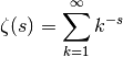
-
double gsl_sf_zeta_int(int n)
-
int gsl_sf_zeta_int_e(int n, gsl_sf_result *result)
These routines compute the Riemann zeta function
 for integer
 n, .
.
-
double gsl_sf_zeta(double s)
-
int gsl_sf_zeta_e(double s, gsl_sf_result *result)
These routines compute the Riemann zeta function
 for arbitrary
 s, .
.
Riemann Zeta Function Minus One
For large positive argument, the Riemann zeta function approaches one. In this region the fractional part is interesting, and therefore we need a function to evaluate it explicitly.
-
double gsl_sf_zetam1_int(int n)
-
int gsl_sf_zetam1_int_e(int n, gsl_sf_result *result)
These routines compute
 for integer
 n,.
-
double gsl_sf_zetam1(double s)
-
int gsl_sf_zetam1_e(double s, gsl_sf_result *result)
These routines compute
 for arbitrary
 s,.
Hurwitz Zeta Function
The Hurwitz zeta function is defined by
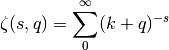
-
double gsl_sf_hzeta(double s, double q)
-
int gsl_sf_hzeta_e(double s, double q, gsl_sf_result *result)
These routines compute the Hurwitz zeta function
 for
for
 ,
,  .
.
Eta Function
The eta function is defined by
-
double gsl_sf_eta_int(int n)
-
int gsl_sf_eta_int_e(int n, gsl_sf_result *result)
These routines compute the eta function
 for integer
 n.
-
double gsl_sf_eta(double s)
-
int gsl_sf_eta_e(double s, gsl_sf_result *result)
These routines compute the eta function
 for arbitrary
 s.
Examples
The following example demonstrates the use of the error handling form of
the special functions, in this case to compute the Bessel function
 ,
,
#include <stdio.h>
#include <gsl/gsl_errno.h>
#include <gsl/gsl_sf_bessel.h>

int
main (void)
{
  double x = 5.0;
  gsl_sf_result result;

  double expected = -0.17759677131433830434739701;

  int status = gsl_sf_bessel_J0_e (x, &result);

  printf ("status  = %s\n", gsl_strerror(status));
  printf ("J0(5.0) = %.18f\n"
          "      +/- % .18f\n",
          result.val, result.err);
  printf ("exact   = %.18f\n", expected);
  return status;
}
Here are the results of running the program,
status  = success
J0(5.0) = -0.177596771314338264
      +/-  0.000000000000000193
exact   = -0.177596771314338292
The next program computes the same quantity using the natural form of
the function. In this case the error term result.err and return
status are not accessible.
#include <stdio.h>
#include <gsl/gsl_sf_bessel.h>

int
main (void)
{
  double x = 5.0;
  double expected = -0.17759677131433830434739701;

  double y = gsl_sf_bessel_J0 (x);

  printf ("J0(5.0) = %.18f\n", y);
  printf ("exact   = %.18f\n", expected);
  return 0;
}
The results of the function are the same,
J0(5.0) = -0.177596771314338264
exact   = -0.177596771314338292
References and Further Reading
The library follows the conventions of the following book where possible,
Handbook of Mathematical Functions, edited by Abramowitz & Stegun, Dover, ISBN 0486612724.
The following papers contain information on the algorithms used to compute the special functions,
Allan J. MacLeod, MISCFUN: A software package to compute uncommon special functions. ACM Trans. Math. Soft., vol.: 22, 1996, 288–301
Bunck, B. F., A fast algorithm for evaluation of normalized Hermite functions, BIT Numer. Math, 49: 281-295, 2009.
G.N. Watson, A Treatise on the Theory of Bessel Functions, 2nd Edition (Cambridge University Press, 1944).
G. Nemeth, Mathematical Approximations of Special Functions, Nova Science Publishers, ISBN 1-56072-052-2
B.C. Carlson, Special Functions of Applied Mathematics (1977)
N. M. Temme, Special Functions: An Introduction to the Classical Functions of Mathematical Physics (1996), ISBN 978-0471113133.
W.J. Thompson, Atlas for Computing Mathematical Functions, John Wiley & Sons, New York (1997).
Y.Y. Luke, Algorithms for the Computation of Mathematical Functions, Academic Press, New York (1977).
S. A. Holmes and W. E. Featherstone, A unified approach to the Clenshaw summation and the recursive computation of very high degree and order normalised associated Legendre functions, Journal of Geodesy, 76, pg. 279-299, 2002.