Statistics¶

This chapter describes the statistical functions in the library. The basic statistical functions include routines to compute the mean, variance and standard deviation. More advanced functions allow you to calculate absolute deviations, skewness, and kurtosis as well as the median and arbitrary percentiles. The algorithms use recurrence relations to compute average quantities in a stable way, without large intermediate values that might overflow.

The functions are available in versions for datasets in the standard floating-point and integer types. The versions for double precision floating-point data have the prefix gsl_stats and are declared in the header file gsl_statistics_double.h. The versions for integer data have the prefix gsl_stats_int and are declared in the header file gsl_statistics_int.h. All the functions operate on C arrays with a stride parameter specifying the spacing between elements.

Mean, Standard Deviation and Variance¶

double gsl_stats_mean(const double data[], size_t stride, size_t n)¶

This function returns the arithmetic mean of data, a dataset of length n with stride stride. The arithmetic mean, or sample mean, is denoted by $\Hat\mu$ and defined as,

$\Hat\mu = {1 \over N} \sum x_i$

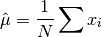
where $x_i$ are the elements of the dataset data. For samples drawn from a gaussian distribution the variance of $\Hat\mu$ is $\sigma^2 / N$ .

double gsl_stats_variance(const double data[], size_t stride, size_t n)¶

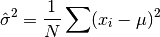
This function returns the estimated, or sample, variance of data, a dataset of length n with stride stride. The estimated variance is denoted by $\Hat\sigma^2$ and is defined by,

${\Hat\sigma}^2 = {1 \over (N-1)} \sum (x_i - {\Hat\mu})^2$

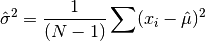
where $x_i$ are the elements of the dataset data. Note that the normalization factor of $1/(N-1)$ results from the derivation of $\Hat\sigma^2$ as an unbiased estimator of the population variance $\sigma^2$ . For samples drawn from a Gaussian distribution the variance of $\Hat\sigma^2$ itself is $2 \sigma^4 / N$ .

This function computes the mean via a call to gsl_stats_mean(). If you have already computed the mean then you can pass it directly to gsl_stats_variance_m().

double gsl_stats_variance_m(const double data[], size_t stride, size_t n, double mean)¶: This function returns the sample variance of data relative to the given value of mean. The function is computed with $\Hat\mu$ replaced by the value of mean that you supply,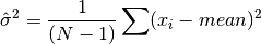

${\Hat\sigma}^2 = {1 \over (N-1)} \sum (x_i - mean)^2$

double gsl_stats_sd(const double data[], size_t stride, size_t n)¶
double gsl_stats_sd_m(const double data[], size_t stride, size_t n, double mean)¶: The standard deviation is defined as the square root of the variance. These functions return the square root of the corresponding variance functions above.

double gsl_stats_tss(const double data[], size_t stride, size_t n)¶
double gsl_stats_tss_m(const double data[], size_t stride, size_t n, double mean)¶: These functions return the total sum of squares (TSS) of data about the mean. For gsl_stats_tss_m() the user-supplied value of mean is used, and for gsl_stats_tss() it is computed using gsl_stats_mean().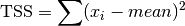

${\rm TSS} = \sum (x_i - mean)^2$

double gsl_stats_variance_with_fixed_mean(const double data[], size_t stride, size_t n, double mean)¶: This function computes an unbiased estimate of the variance of data when the population mean mean of the underlying distribution is known a priori. In this case the estimator for the variance uses the factor $1/N$ and the sample mean $\Hat\mu$ is replaced by the known population mean $\mu$ ,

${\Hat\sigma}^2 = {1 \over N} \sum (x_i - \mu)^2$

double gsl_stats_sd_with_fixed_mean(const double data[], size_t stride, size_t n, double mean)¶: This function calculates the standard deviation of data for a fixed population mean mean. The result is the square root of the corresponding variance function.

Absolute deviation¶

double gsl_stats_absdev(const double data[], size_t stride, size_t n)¶

This function computes the absolute deviation from the mean of data, a dataset of length n with stride stride. The absolute deviation from the mean is defined as,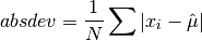

$absdev = {1 \over N} \sum |x_i - {\Hat\mu}|$

where $x_i$ are the elements of the dataset data. The absolute deviation from the mean provides a more robust measure of the width of a distribution than the variance. This function computes the mean of data via a call to gsl_stats_mean().

double gsl_stats_absdev_m(const double data[], size_t stride, size_t n, double mean)¶

This function computes the absolute deviation of the dataset data relative to the given value of mean,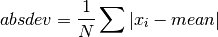

$absdev = {1 \over N} \sum |x_i - mean|$

This function is useful if you have already computed the mean of data (and want to avoid recomputing it), or wish to calculate the absolute deviation relative to another value (such as zero, or the median).

Higher moments (skewness and kurtosis)¶

double gsl_stats_skew(const double data[], size_t stride, size_t n)¶

This function computes the skewness of data, a dataset of length n with stride stride. The skewness is defined as,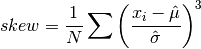

$skew = {1 \over N} \sum {\left( x_i - {\Hat\mu} \over {\Hat\sigma} \right)}^3$

where $x_i$ are the elements of the dataset data. The skewness measures the asymmetry of the tails of a distribution.

The function computes the mean and estimated standard deviation of data via calls to gsl_stats_mean() and gsl_stats_sd().

double gsl_stats_skew_m_sd(const double data[], size_t stride, size_t n, double mean, double sd)¶

This function computes the skewness of the dataset data using the given values of the mean mean and standard deviation sd,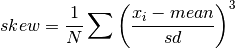

$skew = {1 \over N} \sum {\left( x_i - mean \over sd \right)}^3$

These functions are useful if you have already computed the mean and standard deviation of data and want to avoid recomputing them.

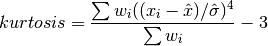
double gsl_stats_kurtosis(const double data[], size_t stride, size_t n)¶

This function computes the kurtosis of data, a dataset of length n with stride stride. The kurtosis is defined as,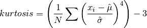

$kurtosis = \left( {1 \over N} \sum {\left(x_i - {\Hat\mu} \over {\Hat\sigma} \right)}^4 \right) - 3$

The kurtosis measures how sharply peaked a distribution is, relative to its width. The kurtosis is normalized to zero for a Gaussian distribution.

double gsl_stats_kurtosis_m_sd(const double data[], size_t stride, size_t n, double mean, double sd)¶

This function computes the kurtosis of the dataset data using the given values of the mean mean and standard deviation sd,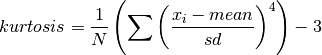

$kurtosis = {1 \over N} \left( \sum {\left(x_i - mean \over sd \right)}^4 \right) - 3$

This function is useful if you have already computed the mean and standard deviation of data and want to avoid recomputing them.

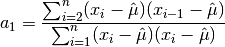
Autocorrelation¶

double gsl_stats_lag1_autocorrelation(const double data[], const size_t stride, const size_t n)¶: This function computes the lag-1 autocorrelation of the dataset data.

$a_1 = {\sum_{i = 2}^{n} (x_{i} - \Hat\mu) (x_{i-1} - \Hat\mu) \over \sum_{i = 1}^{n} (x_{i} - \Hat\mu) (x_{i} - \Hat\mu)}$

double gsl_stats_lag1_autocorrelation_m(const double data[], const size_t stride, const size_t n, const double mean)¶: This function computes the lag-1 autocorrelation of the dataset data using the given value of the mean mean.

Covariance¶

double gsl_stats_covariance(const double data1[], const size_t stride1, const double data2[], const size_t stride2, const size_t n)¶: This function computes the covariance of the datasets data1 and data2 which must both be of the same length n.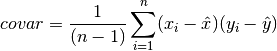

$covar = {1 \over (n - 1)} \sum_{i = 1}^{n} (x_{i} - \Hat x) (y_{i} - \Hat y)$

double gsl_stats_covariance_m(const double data1[], const size_t stride1, const double data2[], const size_t stride2, const size_t n, const double mean1, const double mean2)¶: This function computes the covariance of the datasets data1 and data2 using the given values of the means, mean1 and mean2. This is useful if you have already computed the means of data1 and data2 and want to avoid recomputing them.

Correlation¶

double gsl_stats_correlation(const double data1[], const size_t stride1, const double data2[], const size_t stride2, const size_t n)¶: This function efficiently computes the Pearson correlation coefficient between the datasets data1 and data2 which must both be of the same length n.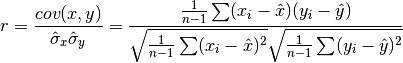

$r = {cov(x, y) \over \Hat\sigma_x \Hat\sigma_y} = {{1 \over n-1} \sum (x_i - \Hat x) (y_i - \Hat y) \over \sqrt{{1 \over n-1} \sum (x_i - {\Hat x})^2} \sqrt{{1 \over n-1} \sum (y_i - {\Hat y})^2} }$

double gsl_stats_spearman(const double data1[], const size_t stride1, const double data2[], const size_t stride2, const size_t n, double work[])¶: This function computes the Spearman rank correlation coefficient between the datasets data1 and data2 which must both be of the same length n. Additional workspace of size 2 * n is required in work. The Spearman rank correlation between vectors $x$ and $y$ is equivalent to the Pearson correlation between the ranked vectors $x_R$ and $y_R$ , where ranks are defined to be the average of the positions of an element in the ascending order of the values.

Weighted Samples¶

The functions described in this section allow the computation of statistics for weighted samples. The functions accept an array of samples, $x_i$ , with associated weights, $w_i$ . Each sample $x_i$ is considered as having been drawn from a Gaussian distribution with variance $\sigma_i^2$ . The sample weight $w_i$ is defined as the reciprocal of this variance, $w_i = 1/\sigma_i^2$ . Setting a weight to zero corresponds to removing a sample from a dataset.

double gsl_stats_wmean(const double w[], size_t wstride, const double data[], size_t stride, size_t n)¶: This function returns the weighted mean of the dataset data with stride stride and length n, using the set of weights w with stride wstride and length n. The weighted mean is defined as,

${\Hat\mu} = {{\sum w_i x_i} \over {\sum w_i}}$

double gsl_stats_wvariance(const double w[], size_t wstride, const double data[], size_t stride, size_t n)¶

This function returns the estimated variance of the dataset data with stride stride and length n, using the set of weights w with stride wstride and length n. The estimated variance of a weighted dataset is calculated as,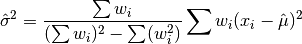

$\Hat\sigma^2 = {{\sum w_i} \over {(\sum w_i)^2 - \sum (w_i^2)}} \sum w_i (x_i - \Hat\mu)^2$

Note that this expression reduces to an unweighted variance with the familiar $1/(N-1)$ factor when there are $N$ equal non-zero weights.

double gsl_stats_wvariance_m(const double w[], size_t wstride, const double data[], size_t stride, size_t n, double wmean)¶: This function returns the estimated variance of the weighted dataset data using the given weighted mean wmean.

double gsl_stats_wsd(const double w[], size_t wstride, const double data[], size_t stride, size_t n)¶: The standard deviation is defined as the square root of the variance. This function returns the square root of the corresponding variance function gsl_stats_wvariance() above.

double gsl_stats_wsd_m(const double w[], size_t wstride, const double data[], size_t stride, size_t n, double wmean)¶: This function returns the square root of the corresponding variance function gsl_stats_wvariance_m() above.

double gsl_stats_wvariance_with_fixed_mean(const double w[], size_t wstride, const double data[], size_t stride, size_t n, const double mean)¶: This function computes an unbiased estimate of the variance of the weighted dataset data when the population mean mean of the underlying distribution is known a priori. In this case the estimator for the variance replaces the sample mean $\Hat\mu$ by the known population mean 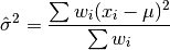$\mu$ ,

$\Hat\sigma^2 = {{\sum w_i (x_i - \mu)^2} \over {\sum w_i}}$

double gsl_stats_wsd_with_fixed_mean(const double w[], size_t wstride, const double data[], size_t stride, size_t n, const double mean)¶: The standard deviation is defined as the square root of the variance. This function returns the square root of the corresponding variance function above.

double gsl_stats_wtss(const double w[], const size_t wstride, const double data[], size_t stride, size_t n)¶
double gsl_stats_wtss_m(const double w[], const size_t wstride, const double data[], size_t stride, size_t n, double wmean)¶: These functions return the weighted total sum of squares (TSS) of data about the weighted mean. For gsl_stats_wtss_m() the user-supplied value of wmean is used, and for gsl_stats_wtss() it is computed using gsl_stats_wmean().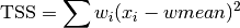

${\rm TSS} = \sum w_i (x_i - wmean)^2$

double gsl_stats_wabsdev(const double w[], size_t wstride, const double data[], size_t stride, size_t n)¶: This function computes the weighted absolute deviation from the weighted mean of data. The absolute deviation from the mean is defined as,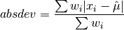

$absdev = {{\sum w_i |x_i - \Hat\mu|} \over {\sum w_i}}$

double gsl_stats_wabsdev_m(const double w[], size_t wstride, const double data[], size_t stride, size_t n, double wmean)¶: This function computes the absolute deviation of the weighted dataset data about the given weighted mean wmean.

double gsl_stats_wskew(const double w[], size_t wstride, const double data[], size_t stride, size_t n)¶: This function computes the weighted skewness of the dataset data.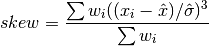

$skew = {{\sum w_i ((x_i - {\Hat x})/{\Hat \sigma})^3} \over {\sum w_i}}$

double gsl_stats_wskew_m_sd(const double w[], size_t wstride, const double data[], size_t stride, size_t n, double wmean, double wsd)¶: This function computes the weighted skewness of the dataset data using the given values of the weighted mean and weighted standard deviation, wmean and wsd.

double gsl_stats_wkurtosis(const double w[], size_t wstride, const double data[], size_t stride, size_t n)¶: This function computes the weighted kurtosis of the dataset data.

$kurtosis = {{\sum w_i ((x_i - {\Hat x})/{\Hat \sigma})^4} \over {\sum w_i}} - 3$

double gsl_stats_wkurtosis_m_sd(const double w[], size_t wstride, const double data[], size_t stride, size_t n, double wmean, double wsd)¶: This function computes the weighted kurtosis of the dataset data using the given values of the weighted mean and weighted standard deviation, wmean and wsd.

Maximum and Minimum values¶

The following functions find the maximum and minimum values of a dataset (or their indices). If the data contains NaN-s then a NaN will be returned, since the maximum or minimum value is undefined. For functions which return an index, the location of the first NaN in the array is returned.

double gsl_stats_max(const double data[], size_t stride, size_t n)¶

This function returns the maximum value in data, a dataset of length n with stride stride. The maximum value is defined as the value of the element $x_i$ which satisfies $x_i \ge x_j$ for all $j$ .

If you want instead to find the element with the largest absolute magnitude you will need to apply fabs() or abs() to your data before calling this function.

double gsl_stats_min(const double data[], size_t stride, size_t n)¶

This function returns the minimum value in data, a dataset of length n with stride stride. The minimum value is defined as the value of the element $x_i$ which satisfies $x_i \le x_j$ for all $j$ .

If you want instead to find the element with the smallest absolute magnitude you will need to apply fabs() or abs() to your data before calling this function.

void gsl_stats_minmax(double *min, double *max, const double data[], size_t stride, size_t n)¶: This function finds both the minimum and maximum values min, max in data in a single pass.

size_t gsl_stats_max_index(const double data[], size_t stride, size_t n)¶: This function returns the index of the maximum value in data, a dataset of length n with stride stride. The maximum value is defined as the value of the element $x_i$ which satisfies $x_i \ge x_j$ for all $j$ . When there are several equal maximum elements then the first one is chosen.

size_t gsl_stats_min_index(const double data[], size_t stride, size_t n)¶: This function returns the index of the minimum value in data, a dataset of length n with stride stride. The minimum value is defined as the value of the element $x_i$ which satisfies $x_i \ge x_j$ for all $j$ . When there are several equal minimum elements then the first one is chosen.

void gsl_stats_minmax_index(size_t *min_index, size_t *max_index, const double data[], size_t stride, size_t n)¶: This function returns the indexes min_index, max_index of the minimum and maximum values in data in a single pass.

Median and Percentiles¶

The median and percentile functions described in this section operate on sorted data in $O(1)$ time. There is also a routine for computing the median of an unsorted input array in average $O(n)$ time using the quickselect algorithm. For convenience we use quantiles, measured on a scale of 0 to 1, instead of percentiles (which use a scale of 0 to 100).

double gsl_stats_median_from_sorted_data(const double sorted_data[], const size_t stride, const size_t n)¶

This function returns the median value of sorted_data, a dataset of length n with stride stride. The elements of the array must be in ascending numerical order. There are no checks to see whether the data are sorted, so the function gsl_sort() should always be used first.

When the dataset has an odd number of elements the median is the value of element $(n-1)/2$ . When the dataset has an even number of elements the median is the mean of the two nearest middle values, elements $(n-1)/2$ and $n/2$ . Since the algorithm for computing the median involves interpolation this function always returns a floating-point number, even for integer data types.

double gsl_stats_median(double data[], const size_t stride, const size_t n)¶: This function returns the median value of data, a dataset of length n with stride stride. The median is found using the quickselect algorithm. The input array does not need to be sorted, but note that the algorithm rearranges the array and so the input is not preserved on output.

double gsl_stats_quantile_from_sorted_data(const double sorted_data[], size_t stride, size_t n, double f)¶

This function returns a quantile value of sorted_data, a double-precision array of length n with stride stride. The elements of the array must be in ascending numerical order. The quantile is determined by the f, a fraction between 0 and 1. For example, to compute the value of the 75th percentile f should have the value 0.75.

There are no checks to see whether the data are sorted, so the function gsl_sort() should always be used first.

The quantile is found by interpolation, using the formula

$\hbox{quantile} = (1 - \delta) x_i + \delta x_{i+1}$

where $i$ is floor((n - 1)f) and $\delta$ is $(n-1)f - i$ .

Thus the minimum value of the array (data[0*stride]) is given by f equal to zero, the maximum value (data[(n-1)*stride]) is given by f equal to one and the median value is given by f equal to 0.5. Since the algorithm for computing quantiles involves interpolation this function always returns a floating-point number, even for integer data types.

Order Statistics¶

The $k$ -th order statistic of a sample is equal to its $k$ -th smallest value. The $k$ -th order statistic of a set of $n$ values $x = \left\{ x_i \right\}, 1 \le i \le n$ is denoted $x_{(k)}$ . The median of the set $x$ is equal to $x_{\left( \frac{n}{2} \right)}$ if $n$ is odd, or the average of $x_{\left( \frac{n}{2} \right)}$ and $x_{\left( \frac{n}{2} + 1 \right)}$ if $n$ is even. The $k$ -th smallest element of a length $n$ vector can be found in average $O(n)$ time using the quickselect algorithm.

double gsl_stats_select(double data[], const size_t stride, const size_t n, const size_t k)¶: This function finds the k-th smallest element of the input array data of length n and stride stride using the quickselect method. The algorithm rearranges the elements of data and so the input array is not preserved on output.

Robust Location Estimates¶

A location estimate refers to a typical or central value which best describes a given dataset. The mean and median are both examples of location estimators. However, the mean has a severe sensitivity to data outliers and can give erroneous values when even a small number of outliers are present. The median on the other hand, has a strong insensitivity to data outliers, but due to its non-smoothness it can behave unexpectedly in certain situations. GSL offers the following alternative location estimators, which are robust to the presence of outliers.

Trimmed Mean¶

The trimmed mean, or truncated mean, discards a certain number of smallest and largest samples from the input vector before computing the mean of the remaining samples. The amount of trimming is specified by a factor $\alpha \in [0,0.5]$ . Then the number of samples discarded from both ends of the input vector is $\left\lfloor \alpha n \right\rfloor$ , where $n$ is the length of the input. So to discard 25% of the samples from each end, one would set $\alpha = 0.25$ .

double gsl_stats_trmean_from_sorted_data(const double alpha, const double sorted_data[], const size_t stride, const size_t n)¶: This function returns the trimmed mean of sorted_data, a dataset of length n with stride stride. The elements of the array must be in ascending numerical order. There are no checks to see whether the data are sorted, so the function gsl_sort() should always be used first. The trimming factor $\alpha$ is given in alpha. If $\alpha \ge 0.5$ , then the median of the input is returned.

Gastwirth Estimator¶

Gastwirth’s location estimator is a weighted sum of three order statistics,

$gastwirth = 0.3 \times Q_{\frac{1}{3}} + 0.4 \times Q_{\frac{1}{2}} + 0.3 \times Q_{\frac{2}{3}}$

where $Q_{\frac{1}{3}}$ is the one-third quantile, $Q_{\frac{1}{2}}$ is the one-half quantile (i.e. median), and $Q_{\frac{2}{3}}$ is the two-thirds quantile.

double gsl_stats_gastwirth_from_sorted_data(const double sorted_data[], const size_t stride, const size_t n)¶: This function returns the Gastwirth location estimator of sorted_data, a dataset of length n with stride stride. The elements of the array must be in ascending numerical order. There are no checks to see whether the data are sorted, so the function gsl_sort() should always be used first.

Robust Scale Estimates¶

A robust scale estimate, also known as a robust measure of scale, attempts to quantify the statistical dispersion (variability, scatter, spread) in a set of data which may contain outliers. In such datasets, the usual variance or standard deviation scale estimate can be rendered useless by even a single outlier.

Median Absolute Deviation (MAD)¶

The median absolute deviation (MAD) is defined as

$MAD = 1.4826 \times \textrm{median} \left\{ \left| x_i - \textrm{median} \left( x \right) \right| \right\}$

In words, first the median of all samples is computed. Then the median is subtracted from all samples in the input to find the deviation of each sample from the median. The median of all absolute deviations is then the MAD. The factor $1.4826$ makes the MAD an unbiased estimator of the standard deviation for Gaussian data. The median absolute deviation has an asymptotic efficiency of 37%.

double gsl_stats_mad0(const double data[], const size_t stride, const size_t n, double work[])¶

double gsl_stats_mad(const double data[], const size_t stride, const size_t n, double work[])¶: These functions return the median absolute deviation of data, a dataset of length n and stride stride. The mad0 function calculates $\textrm{median} \left\{ \left| x_i - \textrm{median} \left( x \right) \right| \right\}$ (i.e. the $MAD$ statistic without the bias correction scale factor). These functions require additional workspace of size n provided in work.

$S_n$ Statistic¶

The $S_n$ statistic developed by Croux and Rousseeuw is defined as

$S_n = 1.1926 \times c_n \times \textrm{median}_i \left\{ \textrm{median}_j \left( \left| x_i - x_j \right| \right) \right\}$

For each sample $x_i, 1 \le i \le n$ , the median of the values $\left| x_i - x_j \right|$ is computed for all $x_j, 1 \le j \le n$ . This yields $n$ values, whose median then gives the final $S_n$ . The factor $1.1926$ makes $S_n$ an unbiased estimate of the standard deviation for Gaussian data. The factor $c_n$ is a correction factor to correct bias in small sample sizes. $S_n$ has an asymptotic efficiency of 58%.

double gsl_stats_Sn0_from_sorted_data(const double sorted_data[], const size_t stride, const size_t n, double work[])¶

double gsl_stats_Sn_from_sorted_data(const double sorted_data[], const size_t stride, const size_t n, double work[])¶: These functions return the $S_n$ statistic of sorted_data, a dataset of length n with stride stride. The elements of the array must be in ascending numerical order. There are no checks to see whether the data are sorted, so the function gsl_sort() should always be used first. The Sn0 function calculates $\textrm{median}_i \left\{ \textrm{median}_j \left( \left| x_i - x_j \right| \right) \right\}$ (i.e. the $S_n$ statistic without the bias correction scale factors). These functions require additional workspace of size n provided in work.

$Q_n$ Statistic¶

The $Q_n$ statistic developed by Croux and Rousseeuw is defined as

$Q_n = 2.21914 \times d_n \times \left\{ \left| x_i - x_j \right|, i < j \right\}_{(k)}$

The factor $2.21914$ makes $Q_n$ an unbiased estimate of the standard deviation for Gaussian data. The factor $d_n$ is a correction factor to correct bias in small sample sizes. The order statistic is

$k = \left( \begin{array}{c} \left\lfloor \frac{n}{2} \right\rfloor + 1 \\ 2 \end{array} \right)$

$Q_n$ has an asymptotic efficiency of 82%.

double gsl_stats_Qn0_from_sorted_data(const double sorted_data[], const size_t stride, const size_t n, double work[], int work_int[])¶
double gsl_stats_Qn_from_sorted_data(const double sorted_data[], const size_t stride, const size_t n, double work[], int work_int[])¶: These functions return the $Q_n$ statistic of sorted_data, a dataset of length n with stride stride. The elements of the array must be in ascending numerical order. There are no checks to see whether the data are sorted, so the function gsl_sort() should always be used first. The Qn0 function calculates $\left\{ \left| x_i - x_j \right|, i < j \right\}_{(k)}$ (i.e. $Q_n$ without the bias correction scale factors). These functions require additional workspace of size 3n provided in work and integer workspace of size 5n provided in work_int.

Examples¶

Here is a basic example of how to use the statistical functions:

#include <stdio.h>
#include <gsl/gsl_statistics.h>

int
main(void)
{
  double data[5] = {17.2, 18.1, 16.5, 18.3, 12.6};
  double mean, variance, largest, smallest;

  mean     = gsl_stats_mean(data, 1, 5);
  variance = gsl_stats_variance(data, 1, 5);
  largest  = gsl_stats_max(data, 1, 5);
  smallest = gsl_stats_min(data, 1, 5);

  printf ("The dataset is %g, %g, %g, %g, %g\n",
         data[0], data[1], data[2], data[3], data[4]);

  printf ("The sample mean is %g\n", mean);
  printf ("The estimated variance is %g\n", variance);
  printf ("The largest value is %g\n", largest);
  printf ("The smallest value is %g\n", smallest);
  return 0;
}

The program should produce the following output,

The dataset is 17.2, 18.1, 16.5, 18.3, 12.6
The sample mean is 16.54
The estimated variance is 5.373
The largest value is 18.3
The smallest value is 12.6

Here is an example using sorted data,

#include <stdio.h>
#include <gsl/gsl_sort.h>
#include <gsl/gsl_statistics.h>

int
main(void)
{
  double data[5] = {17.2, 18.1, 16.5, 18.3, 12.6};
  double median, upperq, lowerq;

  printf ("Original dataset:  %g, %g, %g, %g, %g\n",
         data[0], data[1], data[2], data[3], data[4]);

  gsl_sort (data, 1, 5);

  printf ("Sorted dataset: %g, %g, %g, %g, %g\n",
         data[0], data[1], data[2], data[3], data[4]);

  median
    = gsl_stats_median_from_sorted_data (data,
                                         1, 5);

  upperq
    = gsl_stats_quantile_from_sorted_data (data,
                                           1, 5,
                                           0.75);
  lowerq
    = gsl_stats_quantile_from_sorted_data (data,
                                           1, 5,
                                           0.25);

  printf ("The median is %g\n", median);
  printf ("The upper quartile is %g\n", upperq);
  printf ("The lower quartile is %g\n", lowerq);
  return 0;
}

This program should produce the following output,

Original dataset:  17.2, 18.1, 16.5, 18.3, 12.6
Sorted dataset: 12.6, 16.5, 17.2, 18.1, 18.3
The median is 17.2
The upper quartile is 18.1
The lower quartile is 16.5

References and Further Reading¶

The standard reference for almost any topic in statistics is the multi-volume Advanced Theory of Statistics by Kendall and Stuart.

Maurice Kendall, Alan Stuart, and J. Keith Ord. The Advanced Theory of Statistics (multiple volumes) reprinted as Kendall’s Advanced Theory of Statistics. Wiley, ISBN 047023380X.

Many statistical concepts can be more easily understood by a Bayesian approach. The following book by Gelman, Carlin, Stern and Rubin gives a comprehensive coverage of the subject.

Andrew Gelman, John B. Carlin, Hal S. Stern, Donald B. Rubin. Bayesian Data Analysis. Chapman & Hall, ISBN 0412039915.

For physicists the Particle Data Group provides useful reviews of Probability and Statistics in the “Mathematical Tools” section of its Annual Review of Particle Physics.

Review of Particle Properties, R.M. Barnett et al., Physical Review D54, 1 (1996)

The Review of Particle Physics is available online at the website http://pdg.lbl.gov/.

The following papers describe robust scale estimation,

C. Croux and P. J. Rousseeuw, Time-Efficient algorithms for two highly robust estimators of scale, Comp. Stat., Physica, Heidelberg, 1992.
P. J. Rousseeuw and C. Croux, Explicit scale estimators with high breakdown point, L1-Statistical Analysis and Related Methods, pp. 77-92, 1992.