Random Number Distributions
This chapter describes functions for generating random variates and computing their probability distributions. Samples from the distributions described in this chapter can be obtained using any of the random number generators in the library as an underlying source of randomness.
In the simplest cases a non-uniform distribution can be obtained analytically from the uniform distribution of a random number generator by applying an appropriate transformation. This method uses one call to the random number generator. More complicated distributions are created by the acceptance-rejection method, which compares the desired distribution against a distribution which is similar and known analytically. This usually requires several samples from the generator.
The library also provides cumulative distribution functions and inverse cumulative distribution functions, sometimes referred to as quantile functions. The cumulative distribution functions and their inverses are computed separately for the upper and lower tails of the distribution, allowing full accuracy to be retained for small results.
The functions for random variates and probability density functions
described in this section are declared in gsl_randist.h. The
corresponding cumulative distribution functions are declared in
gsl_cdf.h.
Note that the discrete random variate functions always
return a value of type unsigned int, and on most platforms this
has a maximum value of
They should only be called with a safe range of parameters (where there is a negligible probability of a variate exceeding this limit) to prevent incorrect results due to overflow.
Introduction
Continuous random number distributions are defined by a probability
density function,  , such that the probability of
  occurring in the infinitesimal range to
  is
is
 .
.
The cumulative distribution function for the lower tail  is
defined by the integral,
is
defined by the integral,
and gives the probability of a variate taking a value less than .
The cumulative distribution function for the upper tail  is
defined by the integral,
is
defined by the integral,
and gives the probability of a variate taking a value greater than .
The upper and lower cumulative distribution functions are related by
 and satisfy
  ,
,
 .
.
The inverse cumulative distributions,  and
and  give the values of
which correspond to a specific value of
give the values of
which correspond to a specific value of  or
or  .
They can be used to find confidence limits from probability values.
.
They can be used to find confidence limits from probability values.
For discrete distributions the probability of sampling the integer
value  is given by
  , where
  .
The cumulative distribution for the lower tail
.
The cumulative distribution for the lower tail  of a
discrete distribution is defined as,
of a
discrete distribution is defined as,
where the sum is over the allowed range of the distribution less than
or equal to .
The cumulative distribution for the upper tail of a discrete
distribution  is defined as
giving the sum of probabilities for all values greater than .
These two definitions satisfy the identity  .
.
If the range of the distribution is 1 to  inclusive then
 ,
,  while
while  ,
,
 .
.
The Gaussian Distribution
-
double gsl_ran_gaussian(const gsl_rng *r, double sigma)
This function returns a Gaussian random variate, with mean zero and standard deviation
sigma. The probability distribution for Gaussian random variates is,
for
in the range  to
to  . Use the
transformation
. Use the
transformation  on the numbers returned by
gsl_ran_gaussian()to obtain a Gaussian distribution with mean . This function uses the Box-Muller algorithm which requires two
calls to the random number generator
. This function uses the Box-Muller algorithm which requires two
calls to the random number generator r.
-
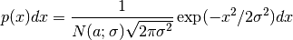
double gsl_ran_gaussian_pdf(double x, double sigma)
This function computes the probability density
at xfor a Gaussian distribution with standard deviationsigma, using the formula given above.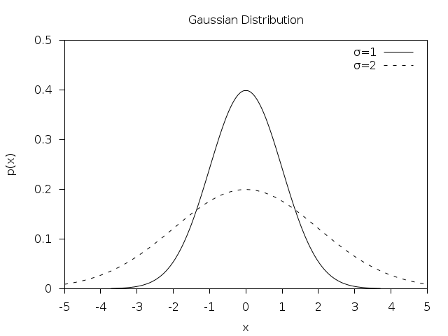
-
double gsl_ran_gaussian_ziggurat(const gsl_rng *r, double sigma)
-
double gsl_ran_gaussian_ratio_method(const gsl_rng *r, double sigma)
This function computes a Gaussian random variate using the alternative Marsaglia-Tsang ziggurat and Kinderman-Monahan-Leva ratio methods. The Ziggurat algorithm is the fastest available algorithm in most cases.
-
double gsl_ran_ugaussian(const gsl_rng *r)
-
double gsl_ran_ugaussian_pdf(double x)
-
double gsl_ran_ugaussian_ratio_method(const gsl_rng *r)
These functions compute results for the unit Gaussian distribution. They are equivalent to the functions above with a standard deviation of one,
sigma= 1.
-
double gsl_cdf_gaussian_P(double x, double sigma)
-
double gsl_cdf_gaussian_Q(double x, double sigma)
-
double gsl_cdf_gaussian_Pinv(double P, double sigma)
-
double gsl_cdf_gaussian_Qinv(double Q, double sigma)
These functions compute the cumulative distribution functions
, and their inverses for the Gaussian
distribution with standard deviation sigma.
The Gaussian Tail Distribution
-
double gsl_ran_gaussian_tail(const gsl_rng *r, double a, double sigma)
This function provides random variates from the upper tail of a Gaussian distribution with standard deviation
sigma. The values returned are larger than the lower limita, which must be positive. The method is based on Marsaglia’s famous rectangle-wedge-tail algorithm (Ann. Math. Stat. 32, 894–899 (1961)), with this aspect explained in Knuth, v2, 3rd ed, p139,586 (exercise 11).The probability distribution for Gaussian tail random variates is,
for
 where
where  is the normalization constant,
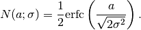
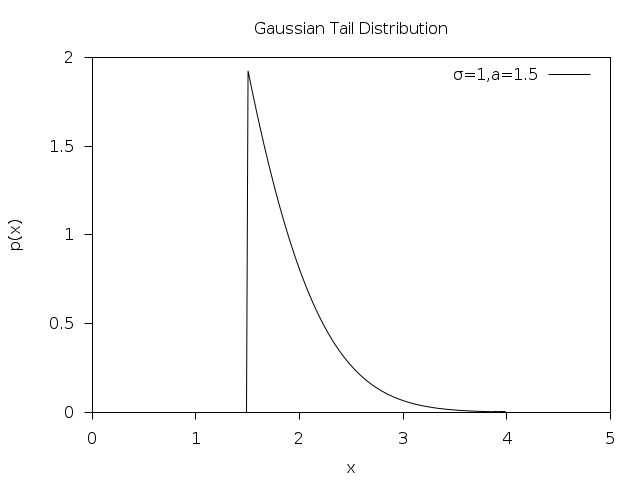
The Bivariate Gaussian Distribution
-
void gsl_ran_bivariate_gaussian(const gsl_rng *r, double sigma_x, double sigma_y, double rho, double *x, double *y)
This function generates a pair of correlated Gaussian variates, with mean zero, correlation coefficient
rhoand standard deviationssigma_xandsigma_yin the and  directions.
The probability distribution for bivariate Gaussian random variates is,
directions.
The probability distribution for bivariate Gaussian random variates is,
for
 in the range to . The
correlation coefficient
in the range to . The
correlation coefficient rhoshould lie between and
and
 .
.
-
double gsl_ran_bivariate_gaussian_pdf(double x, double y, double sigma_x, double sigma_y, double rho)
This function computes the probability density
 at
(
at
(x,y) for a bivariate Gaussian distribution with standard deviationssigma_x,sigma_yand correlation coefficientrho, using the formula given above.
The Multivariate Gaussian Distribution
-
int gsl_ran_multivariate_gaussian(const gsl_rng *r, const gsl_vector *mu, const gsl_matrix *L, gsl_vector *result)
This function generates a random vector satisfying the
-dimensional multivariate Gaussian
distribution with mean and variance-covariance matrix
 . On input, the -vector is given in
 mu, and the Cholesky factor of the-by- matrix  is
given in the lower triangle of
is
given in the lower triangle of L, as output fromgsl_linalg_cholesky_decomp(). The random vector is stored inresulton output. The probability distribution for multivariate Gaussian random variates is
-
int gsl_ran_multivariate_gaussian_pdf(const gsl_vector *x, const gsl_vector *mu, const gsl_matrix *L, double *result, gsl_vector *work)
-
int gsl_ran_multivariate_gaussian_log_pdf(const gsl_vector *x, const gsl_vector *mu, const gsl_matrix *L, double *result, gsl_vector *work)
These functions compute
or  at the point
 x, using mean vectormuand variance-covariance matrix specified by its Cholesky factorLusing the formula above. Additional workspace of length is required in work.
-
int gsl_ran_multivariate_gaussian_mean(const gsl_matrix *X, gsl_vector *mu_hat)
Given a set of
samples  from a -dimensional multivariate Gaussian distribution,
this function computes the maximum likelihood estimate of the mean of the distribution, given by
from a -dimensional multivariate Gaussian distribution,
this function computes the maximum likelihood estimate of the mean of the distribution, given by
The samples
 are given in the -by- matrix
 X, and the maximum likelihood estimate of the mean is stored inmu_haton output.
-
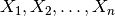
int gsl_ran_multivariate_gaussian_vcov(const gsl_matrix *X, gsl_matrix *sigma_hat)
Given a set of
samples from a -dimensional multivariate Gaussian distribution,
this function computes the maximum likelihood estimate of the variance-covariance matrix of the distribution,
given by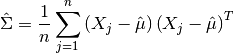
The samples
are given in the -by- matrix Xand the maximum likelihood estimate of the variance-covariance matrix is stored insigma_haton output.
The Exponential Distribution
-
double gsl_ran_exponential(const gsl_rng *r, double mu)
This function returns a random variate from the exponential distribution with mean
mu. The distribution is,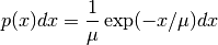
for
 .
.
-
double gsl_ran_exponential_pdf(double x, double mu)
This function computes the probability density
at xfor an exponential distribution with meanmu, using the formula given above.
-
double gsl_cdf_exponential_P(double x, double mu)
-
double gsl_cdf_exponential_Q(double x, double mu)
-
double gsl_cdf_exponential_Pinv(double P, double mu)
-
double gsl_cdf_exponential_Qinv(double Q, double mu)
These functions compute the cumulative distribution functions
, and their inverses for the exponential
distribution with mean mu.
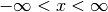
The Laplace Distribution
-
double gsl_ran_laplace(const gsl_rng *r, double a)
This function returns a random variate from the Laplace distribution with width
a. The distribution is,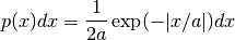
for
 .
.
-
double gsl_ran_laplace_pdf(double x, double a)
This function computes the probability density
at xfor a Laplace distribution with widtha, using the formula given above.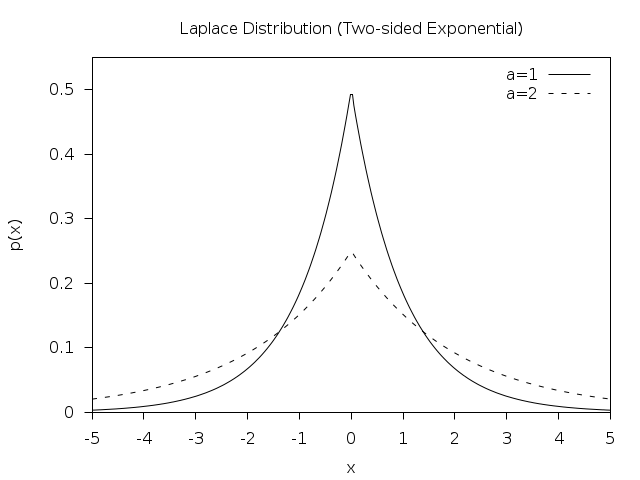
-
double gsl_cdf_laplace_P(double x, double a)
-
double gsl_cdf_laplace_Q(double x, double a)
-
double gsl_cdf_laplace_Pinv(double P, double a)
-
double gsl_cdf_laplace_Qinv(double Q, double a)
These functions compute the cumulative distribution functions
, and their inverses for the Laplace
distribution with width a.
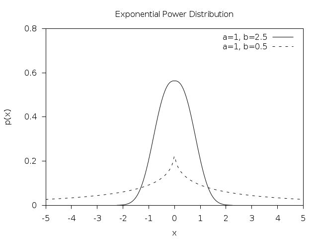
The Exponential Power Distribution
-
double gsl_ran_exppow(const gsl_rng *r, double a, double b)
This function returns a random variate from the exponential power distribution with scale parameter
aand exponentb. The distribution is,
for
.
For  this reduces to the Laplace
distribution. For
this reduces to the Laplace
distribution. For  it has the same form as a Gaussian
distribution, but with
it has the same form as a Gaussian
distribution, but with  .
.
The Cauchy Distribution
-
double gsl_ran_cauchy(const gsl_rng *r, double a)
This function returns a random variate from the Cauchy distribution with scale parameter
a. The probability distribution for Cauchy random variates is,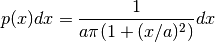
for
in the range to . The Cauchy
distribution is also known as the Lorentz distribution.
-
double gsl_ran_cauchy_pdf(double x, double a)
This function computes the probability density
at xfor a Cauchy distribution with scale parametera, using the formula given above.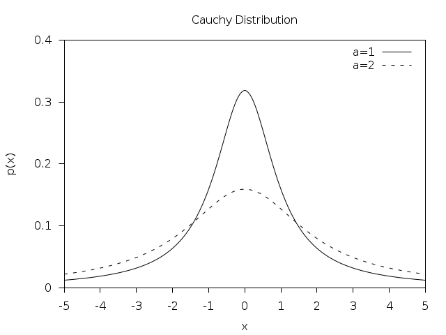
-
double gsl_cdf_cauchy_P(double x, double a)
-
double gsl_cdf_cauchy_Q(double x, double a)
-
double gsl_cdf_cauchy_Pinv(double P, double a)
-
double gsl_cdf_cauchy_Qinv(double Q, double a)
These functions compute the cumulative distribution functions
, and their inverses for the Cauchy
distribution with scale parameter a.
The Rayleigh Distribution
-
double gsl_ran_rayleigh(const gsl_rng *r, double sigma)
This function returns a random variate from the Rayleigh distribution with scale parameter
sigma. The distribution is,
for
 .
.
-
double gsl_ran_rayleigh_pdf(double x, double sigma)
This function computes the probability density
at xfor a Rayleigh distribution with scale parametersigma, using the formula given above.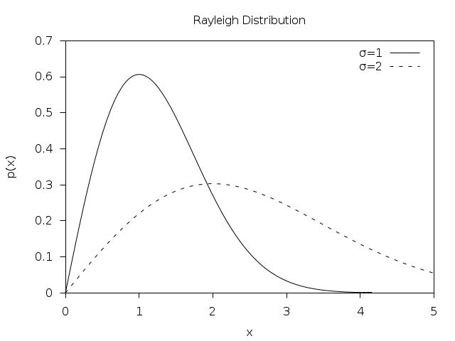
-
double gsl_cdf_rayleigh_P(double x, double sigma)
-
double gsl_cdf_rayleigh_Q(double x, double sigma)
-
double gsl_cdf_rayleigh_Pinv(double P, double sigma)
-
double gsl_cdf_rayleigh_Qinv(double Q, double sigma)
These functions compute the cumulative distribution functions
, and their inverses for the Rayleigh
distribution with scale parameter sigma.
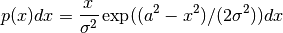
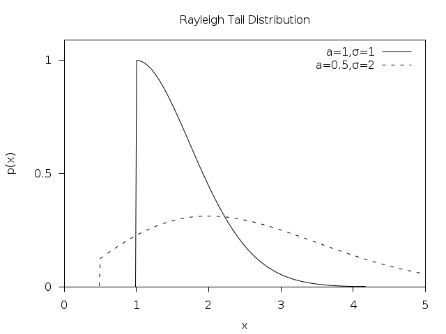
The Rayleigh Tail Distribution
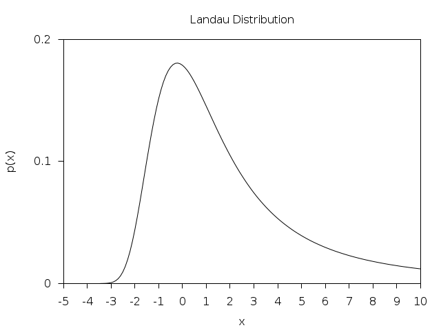
The Landau Distribution
-
double gsl_ran_landau(const gsl_rng *r)
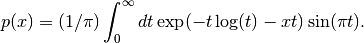
This function returns a random variate from the Landau distribution. The probability distribution for Landau random variates is defined analytically by the complex integral,
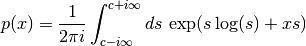
For numerical purposes it is more convenient to use the following equivalent form of the integral,
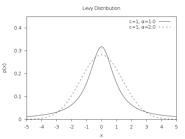
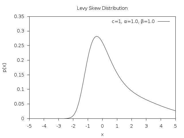
The Levy alpha-Stable Distributions
-
double gsl_ran_levy(const gsl_rng *r, double c, double alpha)
This function returns a random variate from the Levy symmetric stable distribution with scale
cand exponentalpha. The symmetric stable probability distribution is defined by a Fourier transform,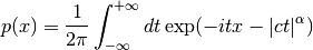
There is no explicit solution for the form of
and the
library does not define a corresponding pdffunction. For the distribution reduces to the Cauchy distribution. For
 it is a Gaussian distribution with
  .
For
.
For  the tails of the distribution become extremely wide.
The algorithm only works for
 .
.
The Levy skew alpha-Stable Distribution
-
double gsl_ran_levy_skew(const gsl_rng *r, double c, double alpha, double beta)
This function returns a random variate from the Levy skew stable distribution with scale
c, exponentalphaand skewness parameterbeta. The skewness parameter must lie in the range![[-1,1]](_images/math/9d7700522727dac61e0f0c6d894326947027e00f.png) . The Levy skew stable probability distribution is defined
by a Fourier transform,
. The Levy skew stable probability distribution is defined
by a Fourier transform,
When
the term  is replaced by
 . There is no explicit solution for the form of
and the library does not define a corresponding
. There is no explicit solution for the form of
and the library does not define a corresponding pdffunction. For the distribution reduces to a Gaussian
distribution with
and the skewness parameter has no effect.
For the tails of the distribution become extremely
wide. The symmetric distribution corresponds to  .
.The algorithm only works for
.
The Levy alpha-stable distributions have the property that if  alpha-stable variates are drawn from the distribution
  then the sum
  will also be
distributed as an alpha-stable variate,
will also be
distributed as an alpha-stable variate,
 .
.
The Gamma Distribution
-
double gsl_ran_gamma(const gsl_rng *r, double a, double b)
This function returns a random variate from the gamma distribution. The distribution function is,
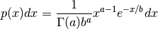
for
.The gamma distribution with an integer parameter
ais known as the Erlang distribution.The variates are computed using the Marsaglia-Tsang fast gamma method. This function for this method was previously called
gsl_ran_gamma_mt()and can still be accessed using this name.
-
double gsl_ran_gamma_knuth(const gsl_rng *r, double a, double b)
This function returns a gamma variate using the algorithms from Knuth (vol 2).
-
double gsl_ran_gamma_pdf(double x, double a, double b)
This function computes the probability density
at xfor a gamma distribution with parametersaandb, using the formula given above.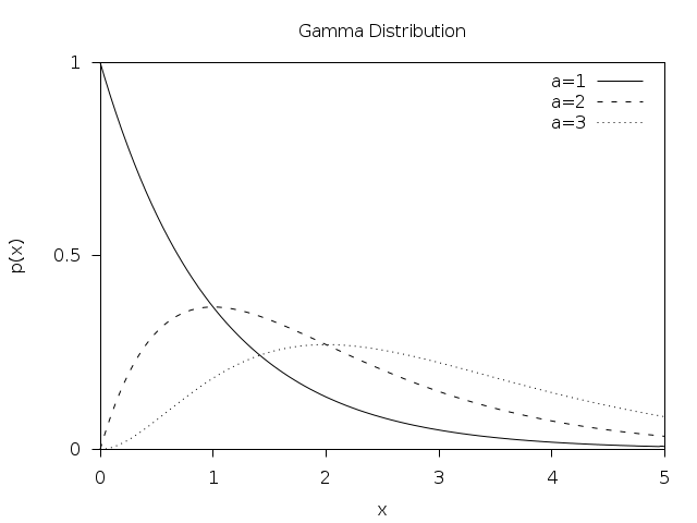
-
double gsl_cdf_gamma_P(double x, double a, double b)
-
double gsl_cdf_gamma_Q(double x, double a, double b)
-
double gsl_cdf_gamma_Pinv(double P, double a, double b)
-
double gsl_cdf_gamma_Qinv(double Q, double a, double b)
These functions compute the cumulative distribution functions
, and their inverses for the gamma
distribution with parameters aandb.
The Flat (Uniform) Distribution
-
double gsl_ran_flat(const gsl_rng *r, double a, double b)
This function returns a random variate from the flat (uniform) distribution from
atob. The distribution is,
if
 and 0 otherwise.
-
double gsl_ran_flat_pdf(double x, double a, double b)
This function computes the probability density
at xfor a uniform distribution fromatob, using the formula given above.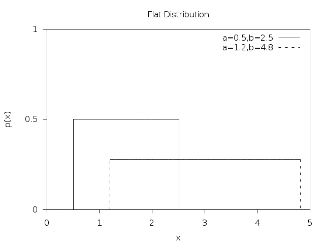
-
double gsl_cdf_flat_P(double x, double a, double b)
-
double gsl_cdf_flat_Q(double x, double a, double b)
-
double gsl_cdf_flat_Pinv(double P, double a, double b)
-
double gsl_cdf_flat_Qinv(double Q, double a, double b)
These functions compute the cumulative distribution functions
, and their inverses for a uniform distribution
from atob.
The Lognormal Distribution
-
double gsl_ran_lognormal(const gsl_rng *r, double zeta, double sigma)
This function returns a random variate from the lognormal distribution. The distribution function is,
for
.
-
double gsl_ran_lognormal_pdf(double x, double zeta, double sigma)
This function computes the probability density
at xfor a lognormal distribution with parameterszetaandsigma, using the formula given above.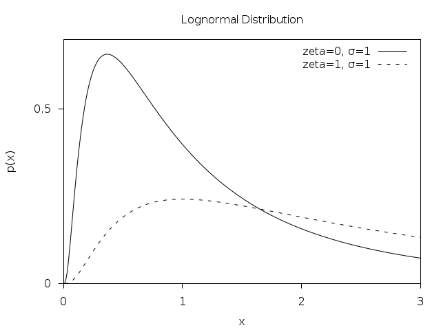
-
double gsl_cdf_lognormal_P(double x, double zeta, double sigma)
-
double gsl_cdf_lognormal_Q(double x, double zeta, double sigma)
-
double gsl_cdf_lognormal_Pinv(double P, double zeta, double sigma)
-
double gsl_cdf_lognormal_Qinv(double Q, double zeta, double sigma)
These functions compute the cumulative distribution functions
, and their inverses for the lognormal
distribution with parameters zetaandsigma.
The Chi-squared Distribution
The chi-squared distribution arises in statistics. If  are
independent Gaussian random variates with unit variance then the
sum-of-squares,
are
independent Gaussian random variates with unit variance then the
sum-of-squares,

has a chi-squared distribution with degrees of freedom.
-
double gsl_ran_chisq(const gsl_rng *r, double nu)
This function returns a random variate from the chi-squared distribution with
nudegrees of freedom. The distribution function is,
for
.
-
double gsl_ran_chisq_pdf(double x, double nu)
This function computes the probability density
at xfor a chi-squared distribution withnudegrees of freedom, using the formula given above.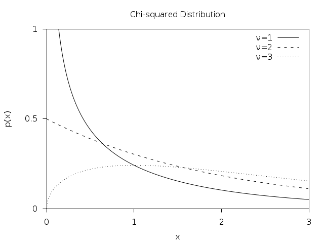
-
double gsl_cdf_chisq_P(double x, double nu)
-
double gsl_cdf_chisq_Q(double x, double nu)
-
double gsl_cdf_chisq_Pinv(double P, double nu)
-
double gsl_cdf_chisq_Qinv(double Q, double nu)
These functions compute the cumulative distribution functions
, and their inverses for the chi-squared
distribution with nudegrees of freedom.
The F-distribution
The F-distribution arises in statistics. If  and
and  are chi-squared deviates with
  and
and  degrees of
freedom then the ratio,
degrees of
freedom then the ratio,

has an F-distribution  .
.
-
double gsl_ran_fdist(const gsl_rng *r, double nu1, double nu2)
This function returns a random variate from the F-distribution with degrees of freedom
nu1andnu2. The distribution function is,
for
.
-
double gsl_ran_fdist_pdf(double x, double nu1, double nu2)
This function computes the probability density
at xfor an F-distribution withnu1andnu2degrees of freedom, using the formula given above.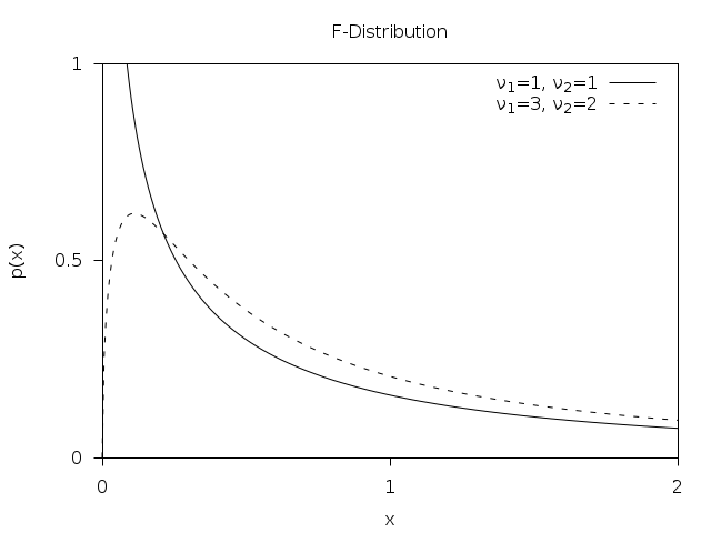
-
double gsl_cdf_fdist_P(double x, double nu1, double nu2)
-
double gsl_cdf_fdist_Q(double x, double nu1, double nu2)
-
double gsl_cdf_fdist_Pinv(double P, double nu1, double nu2)
-
double gsl_cdf_fdist_Qinv(double Q, double nu1, double nu2)
These functions compute the cumulative distribution functions
, and their inverses for the F-distribution
with nu1andnu2degrees of freedom.
The t-distribution
The t-distribution arises in statistics. If has a normal
distribution and has a chi-squared distribution with
 degrees of freedom then the ratio,

has a t-distribution  with degrees of freedom.
-
double gsl_ran_tdist(const gsl_rng *r, double nu)
This function returns a random variate from the t-distribution. The distribution function is,
for
 .
.
-
double gsl_ran_tdist_pdf(double x, double nu)
This function computes the probability density
at xfor a t-distribution withnudegrees of freedom, using the formula given above.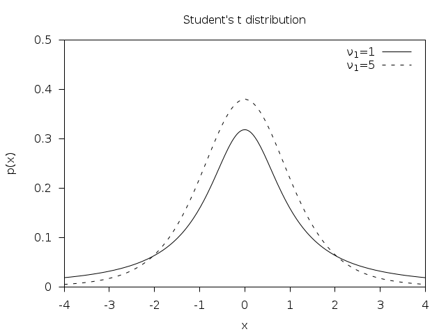
-
double gsl_cdf_tdist_P(double x, double nu)
-
double gsl_cdf_tdist_Q(double x, double nu)
-
double gsl_cdf_tdist_Pinv(double P, double nu)
-
double gsl_cdf_tdist_Qinv(double Q, double nu)
These functions compute the cumulative distribution functions
, and their inverses for the t-distribution
with nudegrees of freedom.
The Beta Distribution
-
double gsl_ran_beta(const gsl_rng *r, double a, double b)
This function returns a random variate from the beta distribution. The distribution function is,
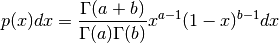
for
 .
.
-
double gsl_ran_beta_pdf(double x, double a, double b)
This function computes the probability density
at xfor a beta distribution with parametersaandb, using the formula given above.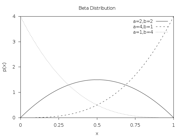
-
double gsl_cdf_beta_P(double x, double a, double b)
-
double gsl_cdf_beta_Q(double x, double a, double b)
-
double gsl_cdf_beta_Pinv(double P, double a, double b)
-
double gsl_cdf_beta_Qinv(double Q, double a, double b)
These functions compute the cumulative distribution functions
, and their inverses for the beta
distribution with parameters aandb.
The Logistic Distribution
-
double gsl_ran_logistic(const gsl_rng *r, double a)
This function returns a random variate from the logistic distribution. The distribution function is,
for
.
-
double gsl_ran_logistic_pdf(double x, double a)
This function computes the probability density
at xfor a logistic distribution with scale parametera, using the formula given above.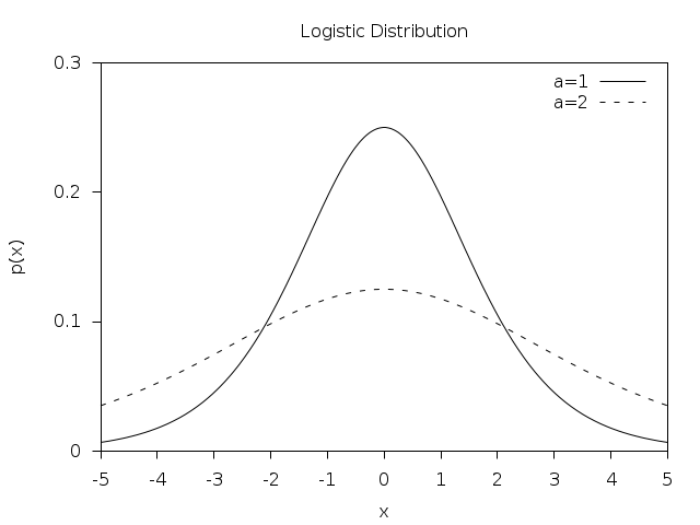
-
double gsl_cdf_logistic_P(double x, double a)
-
double gsl_cdf_logistic_Q(double x, double a)
-
double gsl_cdf_logistic_Pinv(double P, double a)
-
double gsl_cdf_logistic_Qinv(double Q, double a)
These functions compute the cumulative distribution functions
, and their inverses for the logistic
distribution with scale parameter a.
The Pareto Distribution
-
double gsl_ran_pareto(const gsl_rng *r, double a, double b)
This function returns a random variate from the Pareto distribution of order
a. The distribution function is,
for
 .
.
-
double gsl_ran_pareto_pdf(double x, double a, double b)
This function computes the probability density
at xfor a Pareto distribution with exponentaand scaleb, using the formula given above.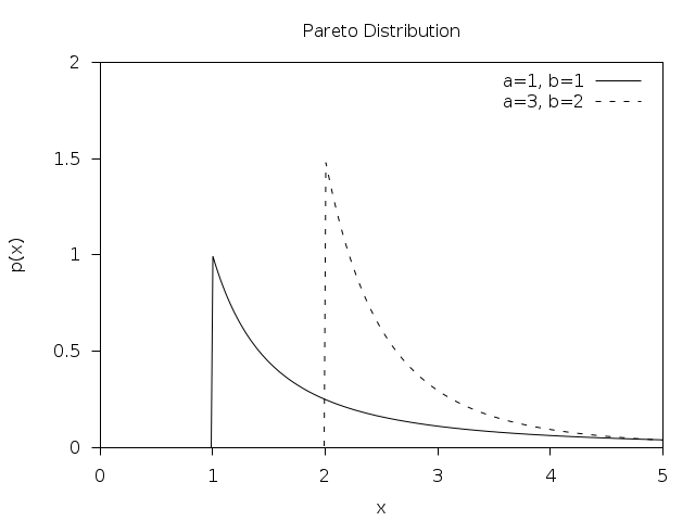
-
double gsl_cdf_pareto_P(double x, double a, double b)
-
double gsl_cdf_pareto_Q(double x, double a, double b)
-
double gsl_cdf_pareto_Pinv(double P, double a, double b)
-
double gsl_cdf_pareto_Qinv(double Q, double a, double b)
These functions compute the cumulative distribution functions
, and their inverses for the Pareto
distribution with exponent aand scaleb.
Spherical Vector Distributions
The spherical distributions generate random vectors, located on a spherical surface. They can be used as random directions, for example in the steps of a random walk.
-
void gsl_ran_dir_2d(const gsl_rng *r, double *x, double *y)
-
void gsl_ran_dir_2d_trig_method(const gsl_rng *r, double *x, double *y)
This function returns a random direction vector
 =
(
=
(x,y) in two dimensions. The vector is normalized such that . The obvious way to do this is to take a
uniform random number between 0 and
. The obvious way to do this is to take a
uniform random number between 0 and  and let
 xandybe the sine and cosine respectively. Two trig functions would have been expensive in the old days, but with modern hardware implementations, this is sometimes the fastest way to go. This is the case for the Pentium (but not the case for the Sun Sparcstation). One can avoid the trig evaluations by choosingxandyin the interior of a unit circle (choose them at random from the interior of the enclosing square, and then reject those that are outside the unit circle), and then dividing by .
A much cleverer approach, attributed to von Neumann (See Knuth, v2, 3rd
ed, p140, exercise 23), requires neither trig nor a square root. In
this approach,
.
A much cleverer approach, attributed to von Neumann (See Knuth, v2, 3rd
ed, p140, exercise 23), requires neither trig nor a square root. In
this approach, uandvare chosen at random from the interior of a unit circle, and then and
and
 .
.
-
void gsl_ran_dir_3d(const gsl_rng *r, double *x, double *y, double *z)
This function returns a random direction vector
=
(x,y,z) in three dimensions. The vector is normalized such that . The method employed is
due to Robert E. Knop (CACM 13, 326 (1970)), and explained in Knuth, v2,
3rd ed, p136. It uses the surprising fact that the distribution
projected along any axis is actually uniform (this is only true for 3
dimensions).
. The method employed is
due to Robert E. Knop (CACM 13, 326 (1970)), and explained in Knuth, v2,
3rd ed, p136. It uses the surprising fact that the distribution
projected along any axis is actually uniform (this is only true for 3
dimensions).
-
void gsl_ran_dir_nd(const gsl_rng *r, size_t n, double *x)
This function returns a random direction vector
 in
in ndimensions. The vector is normalized such that .
The method
uses the fact that a multivariate Gaussian distribution is spherically
symmetric. Each component is generated to have a Gaussian distribution,
and then the components are normalized. The method is described by
Knuth, v2, 3rd ed, p135–136, and attributed to G. W. Brown, Modern
Mathematics for the Engineer (1956).
.
The method
uses the fact that a multivariate Gaussian distribution is spherically
symmetric. Each component is generated to have a Gaussian distribution,
and then the components are normalized. The method is described by
Knuth, v2, 3rd ed, p135–136, and attributed to G. W. Brown, Modern
Mathematics for the Engineer (1956).
The Weibull Distribution
-
double gsl_ran_weibull(const gsl_rng *r, double a, double b)
This function returns a random variate from the Weibull distribution. The distribution function is,
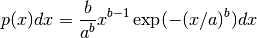
for
.
-
double gsl_ran_weibull_pdf(double x, double a, double b)
This function computes the probability density
at xfor a Weibull distribution with scaleaand exponentb, using the formula given above.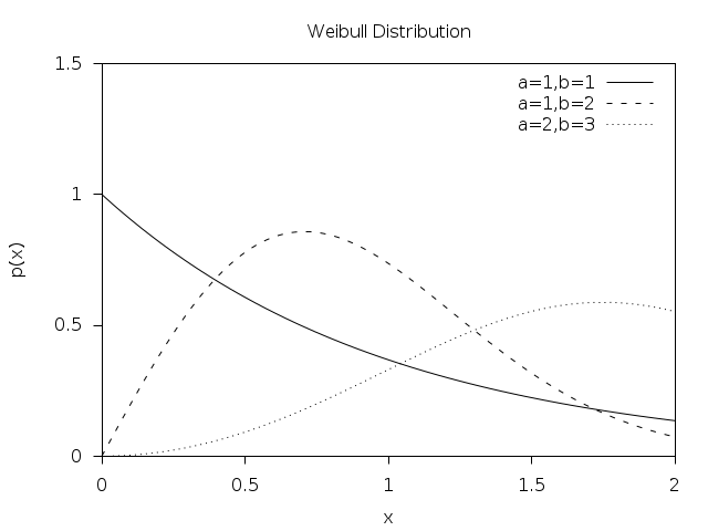
-
double gsl_cdf_weibull_P(double x, double a, double b)
-
double gsl_cdf_weibull_Q(double x, double a, double b)
-
double gsl_cdf_weibull_Pinv(double P, double a, double b)
-
double gsl_cdf_weibull_Qinv(double Q, double a, double b)
These functions compute the cumulative distribution functions
, and their inverses for the Weibull
distribution with scale aand exponentb.
The Type-1 Gumbel Distribution
-
double gsl_ran_gumbel1(const gsl_rng *r, double a, double b)
This function returns a random variate from the Type-1 Gumbel distribution. The Type-1 Gumbel distribution function is,

for
.
-
double gsl_ran_gumbel1_pdf(double x, double a, double b)
This function computes the probability density
at xfor a Type-1 Gumbel distribution with parametersaandb, using the formula given above.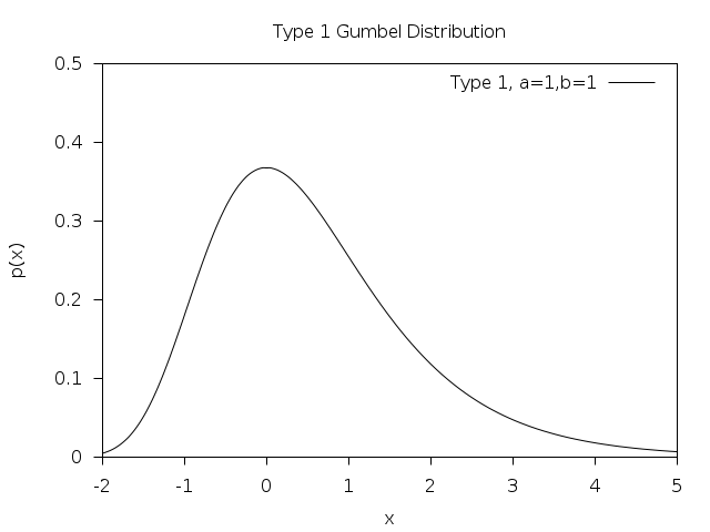
-
double gsl_cdf_gumbel1_P(double x, double a, double b)
-
double gsl_cdf_gumbel1_Q(double x, double a, double b)
-
double gsl_cdf_gumbel1_Pinv(double P, double a, double b)
-
double gsl_cdf_gumbel1_Qinv(double Q, double a, double b)
These functions compute the cumulative distribution functions
, and their inverses for the Type-1 Gumbel
distribution with parameters aandb.
The Type-2 Gumbel Distribution
-
double gsl_ran_gumbel2(const gsl_rng *r, double a, double b)
This function returns a random variate from the Type-2 Gumbel distribution. The Type-2 Gumbel distribution function is,

for
 .
.
-
double gsl_ran_gumbel2_pdf(double x, double a, double b)
This function computes the probability density
at xfor a Type-2 Gumbel distribution with parametersaandb, using the formula given above.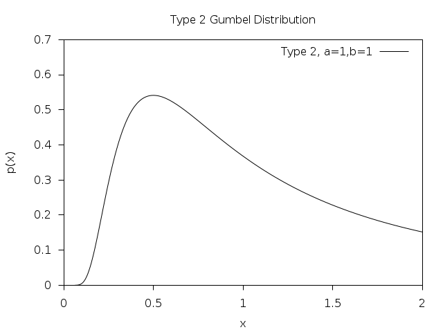
-
double gsl_cdf_gumbel2_P(double x, double a, double b)
-
double gsl_cdf_gumbel2_Q(double x, double a, double b)
-
double gsl_cdf_gumbel2_Pinv(double P, double a, double b)
-
double gsl_cdf_gumbel2_Qinv(double Q, double a, double b)
These functions compute the cumulative distribution functions
, and their inverses for the Type-2 Gumbel
distribution with parameters aandb.
The Dirichlet Distribution
-
void gsl_ran_dirichlet(const gsl_rng *r, size_t K, const double alpha[], double theta[])
This function returns an array of
Krandom variates from a Dirichlet distribution of orderK-1. The distribution function is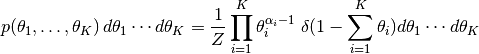
for
 and
and  .
The delta function ensures that
.
The delta function ensures that  .
The normalization factor
.
The normalization factor  is
is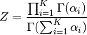
The random variates are generated by sampling
Kvalues from gamma distributions with parameters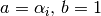 ,
and renormalizing.
See A.M. Law, W.D. Kelton, Simulation Modeling and Analysis (1991).
,
and renormalizing.
See A.M. Law, W.D. Kelton, Simulation Modeling and Analysis (1991).
-
double gsl_ran_dirichlet_pdf(size_t K, const double alpha[], const double theta[])
This function computes the probability density
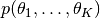 at
at theta[K]for a Dirichlet distribution with parametersalpha[K], using the formula given above.
-
double gsl_ran_dirichlet_lnpdf(size_t K, const double alpha[], const double theta[])
This function computes the logarithm of the probability density
for a Dirichlet distribution with parameters
alpha[K].
General Discrete Distributions
Given  discrete events with different probabilities
 ![P[k]](_images/math/bd166b2bec0ab490649db9232aaaae3d8dd4d47d.png) ,
produce a random value consistent with its probability.
,
produce a random value consistent with its probability.
The obvious way to do this is to preprocess the probability list by
generating a cumulative probability array with  elements:
![C[0] & = 0 \\
C[k+1] &= C[k] + P[k]](_images/math/d530534f8dc817b71950a7115efdef8bf7aedb47.png)
Note that this construction produces ![C[K] = 1](_images/math/e15d942be2ff75681ee7f535e753a30f1a6adcf8.png) . Now choose a
uniform deviate
. Now choose a
uniform deviate  between 0 and 1, and find the value of
such that
between 0 and 1, and find the value of
such that ![C[k] \le u < C[k+1]](_images/math/e3aec9f5e33dfc6b87bf0f09c94fc57adfc15829.png) .
Although this in principle requires of order
.
Although this in principle requires of order  steps per
random number generation, they are fast steps, and if you use something
like
steps per
random number generation, they are fast steps, and if you use something
like  as a starting point, you can often do
pretty well.
as a starting point, you can often do
pretty well.
But faster methods have been devised. Again, the idea is to preprocess
the probability list, and save the result in some form of lookup table;
then the individual calls for a random discrete event can go rapidly.
An approach invented by G. Marsaglia (Generating discrete random variables
in a computer, Comm ACM 6, 37–38 (1963)) is very clever, and readers
interested in examples of good algorithm design are directed to this
short and well-written paper. Unfortunately, for large ,
Marsaglia’s lookup table can be quite large.
A much better approach is due to Alastair J. Walker (An efficient method
for generating discrete random variables with general distributions, ACM
Trans on Mathematical Software 3, 253–256 (1977); see also Knuth, v2,
3rd ed, p120–121,139). This requires two lookup tables, one floating
point and one integer, but both only of size . After
preprocessing, the random numbers are generated in O(1) time, even for
large . The preprocessing suggested by Walker requires
 effort, but that is not actually necessary, and the
implementation provided here only takes
effort, but that is not actually necessary, and the
implementation provided here only takes  effort. In general,
more preprocessing leads to faster generation of the individual random
numbers, but a diminishing return is reached pretty early. Knuth points
out that the optimal preprocessing is combinatorially difficult for
large .
effort. In general,
more preprocessing leads to faster generation of the individual random
numbers, but a diminishing return is reached pretty early. Knuth points
out that the optimal preprocessing is combinatorially difficult for
large .
This method can be used to speed up some of the discrete random number
generators below, such as the binomial distribution. To use it for
something like the Poisson Distribution, a modification would have to
be made, since it only takes a finite set of outcomes.
-
type gsl_ran_discrete_t
This structure contains the lookup table for the discrete random number generator.
-
gsl_ran_discrete_t *gsl_ran_discrete_preproc(size_t K, const double *P)
This function returns a pointer to a structure that contains the lookup table for the discrete random number generator. The array
Pcontains the probabilities of the discrete events; these array elements must all be positive, but they needn’t add up to one (so you can think of them more generally as “weights”)—the preprocessor will normalize appropriately. This return value is used as an argument for thegsl_ran_discrete()function below.
-
size_t gsl_ran_discrete(const gsl_rng *r, const gsl_ran_discrete_t *g)
After the preprocessor, above, has been called, you use this function to get the discrete random numbers.
-
double gsl_ran_discrete_pdf(size_t k, const gsl_ran_discrete_t *g)
Returns the probability
of observing the variable k. Since is not stored as part of the lookup table, it must be
recomputed; this computation takes , so if Kis large and you care about the original array used to create the
lookup table, then you should just keep this original array
around.
-
void gsl_ran_discrete_free(gsl_ran_discrete_t *g)
De-allocates the lookup table pointed to by
g.
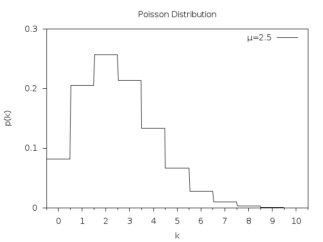
The Poisson Distribution
-
unsigned int gsl_ran_poisson(const gsl_rng *r, double mu)
This function returns a random integer from the Poisson distribution with mean
mu. The probability distribution for Poisson variates is,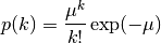
for
 .
.
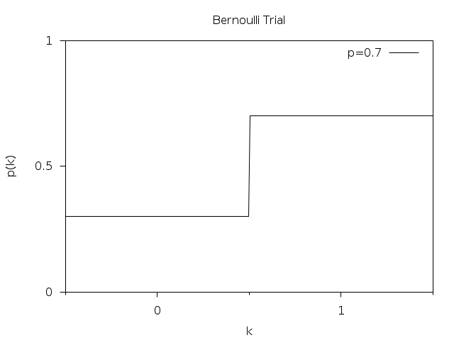
The Bernoulli Distribution

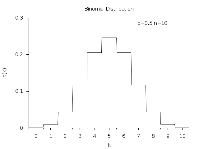
The Binomial Distribution
-
unsigned int gsl_ran_binomial(const gsl_rng *r, double p, unsigned int n)
This function returns a random integer from the binomial distribution, the number of successes in
nindependent trials with probabilityp. The probability distribution for binomial variates is,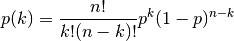
for
 .
.
The Multinomial Distribution
-
void gsl_ran_multinomial(const gsl_rng *r, size_t K, unsigned int N, const double p[], unsigned int n[])
This function computes a random sample
nfrom the multinomial distribution formed byNtrials from an underlying distributionp[K]. The distribution function fornis,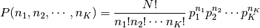
where
 are nonnegative integers with
 ,
and
,
and
 is a probability distribution with
  .
If the array
.
If the array p[K]is not normalized then its entries will be treated as weights and normalized appropriately. The arraysnandpmust both be of lengthK.Random variates are generated using the conditional binomial method (see C.S. Davis, The computer generation of multinomial random variates, Comp. Stat. Data Anal. 16 (1993) 205–217 for details).
-
double gsl_ran_multinomial_pdf(size_t K, const double p[], const unsigned int n[])
This function computes the probability
 of sampling
 n[K]from a multinomial distribution with parametersp[K], using the formula given above.
-
double gsl_ran_multinomial_lnpdf(size_t K, const double p[], const unsigned int n[])
This function returns the logarithm of the probability for the multinomial distribution
with parameters p[K].
The Negative Binomial Distribution
-
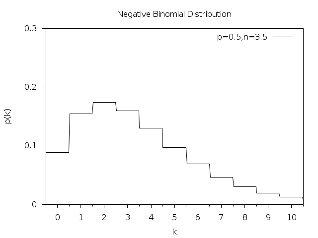
unsigned int gsl_ran_negative_binomial(const gsl_rng *r, double p, double n)
This function returns a random integer from the negative binomial distribution, the number of failures occurring before
nsuccesses in independent trials with probabilitypof success. The probability distribution for negative binomial variates is,
Note that
is not required to be an integer.
The Pascal Distribution
-
unsigned int gsl_ran_pascal(const gsl_rng *r, double p, unsigned int n)
This function returns a random integer from the Pascal distribution. The Pascal distribution is simply a negative binomial distribution with an integer value of
.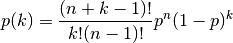
for
.
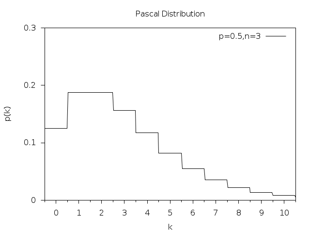
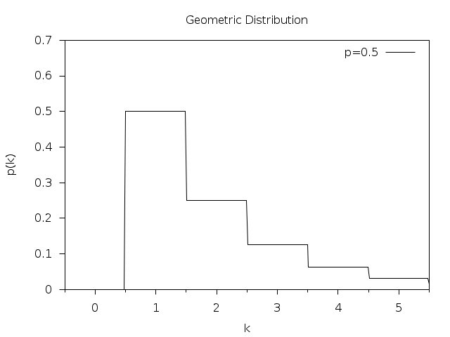
The Geometric Distribution
-
unsigned int gsl_ran_geometric(const gsl_rng *r, double p)
This function returns a random integer from the geometric distribution, the number of independent trials with probability
puntil the first success. The probability distribution for geometric variates is,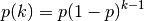
for
 .
Note that the distribution begins with
.
Note that the distribution begins with  with this
definition. There is another convention in which the exponent
with this
definition. There is another convention in which the exponent  is replaced by .
The Hypergeometric Distribution
-
unsigned int gsl_ran_hypergeometric(const gsl_rng *r, unsigned int n1, unsigned int n2, unsigned int t)
This function returns a random integer from the hypergeometric distribution. The probability distribution for hypergeometric random variates is,

where
 and
and
 .
The domain of is
.
The domain of is

If a population contains
 elements of “type 1” and
 elements of “type 2” then the hypergeometric
distribution gives the probability of obtaining elements of
“type 1” in
elements of “type 2” then the hypergeometric
distribution gives the probability of obtaining elements of
“type 1” in  samples from the population without
replacement.
samples from the population without
replacement.
-
double gsl_ran_hypergeometric_pdf(unsigned int k, unsigned int n1, unsigned int n2, unsigned int t)
This function computes the probability
of obtaining kfrom a hypergeometric distribution with parametersn1,n2,t, using the formula given above.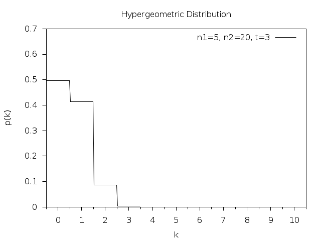
-
double gsl_cdf_hypergeometric_P(unsigned int k, unsigned int n1, unsigned int n2, unsigned int t)
-
double gsl_cdf_hypergeometric_Q(unsigned int k, unsigned int n1, unsigned int n2, unsigned int t)
These functions compute the cumulative distribution functions
, for the hypergeometric distribution with
parameters n1,n2andt.
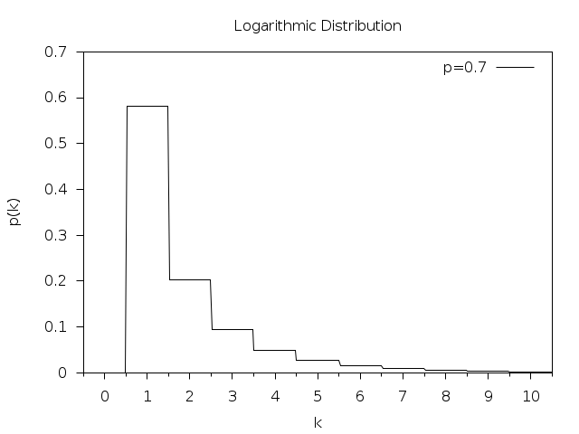
The Logarithmic Distribution
The Wishart Distribution
-
int gsl_ran_wishart(const gsl_rng *r, const double n, const gsl_matrix *L, gsl_matrix *result, gsl_matrix *work)
This function computes a random symmetric
 -by- matrix from the Wishart distribution.
The probability distribution for Wishart random variates is,
-by- matrix from the Wishart distribution.
The probability distribution for Wishart random variates is,
Here,
 is the number of degrees of freedom,
  is a symmetric positive definite
-by- scale matrix, whose Cholesky factor is specified by
is a symmetric positive definite
-by- scale matrix, whose Cholesky factor is specified by L, andworkis-by- workspace. The -by- Wishart distributed matrix  is stored
in
is stored
in resulton output.
-
int gsl_ran_wishart_pdf(const gsl_matrix *X, const gsl_matrix *L_X, const double n, const gsl_matrix *L, double *result, gsl_matrix *work)
-
int gsl_ran_wishart_log_pdf(const gsl_matrix *X, const gsl_matrix *L_X, const double n, const gsl_matrix *L, double *result, gsl_matrix *work)
These functions compute
 or
or  for the -by- matrix
X, whose Cholesky factor is specified inL_X. The degrees of freedom is given byn, the Cholesky factor of the scale matrix is specified in L, andworkis-by- workspace. The probably density value is returned
in result.
Shuffling and Sampling
The following functions allow the shuffling and sampling of a set of objects. The algorithms rely on a random number generator as a source of randomness and a poor quality generator can lead to correlations in the output. In particular it is important to avoid generators with a short period. For more information see Knuth, v2, 3rd ed, Section 3.4.2, “Random Sampling and Shuffling”.
-
void gsl_ran_shuffle(const gsl_rng *r, void *base, size_t n, size_t size)
This function randomly shuffles the order of
nobjects, each of sizesize, stored in the arraybase[0..n-1]. The output of the random number generatorris used to produce the permutation. The algorithm generates all possible permutations with equal probability, assuming a perfect source of random
numbers.
permutations with equal probability, assuming a perfect source of random
numbers.The following code shows how to shuffle the numbers from 0 to 51:
int a[52];

for (i = 0; i < 52; i++)
  {
    a[i] = i;
  }

gsl_ran_shuffle (r, a, 52, sizeof (int));
-
int gsl_ran_choose(const gsl_rng *r, void *dest, size_t k, void *src, size_t n, size_t size)
This function fills the array
dest[k]withkobjects taken randomly from thenelements of the arraysrc[0..n-1]. The objects are each of sizesize. The output of the random number generatorris used to make the selection. The algorithm ensures all possible samples are equally likely, assuming a perfect source of randomness.The objects are sampled without replacement, thus each object can only appear once in
dest. It is required thatkbe less than or equal ton. The objects indestwill be in the same relative order as those insrc. You will need to callgsl_ran_shuffle(r, dest, n, size)if you want to randomize the order.The following code shows how to select a random sample of three unique numbers from the set 0 to 99:
double a[3], b[100];

for (i = 0; i < 100; i++)
  {
    b[i] = (double) i;
  }

gsl_ran_choose (r, a, 3, b, 100, sizeof (double));
-
void gsl_ran_sample(const gsl_rng *r, void *dest, size_t k, void *src, size_t n, size_t size)
This function is like
gsl_ran_choose()but sampleskitems from the original array ofnitemssrcwith replacement, so the same object can appear more than once in the output sequencedest. There is no requirement thatkbe less thannin this case.
Examples
The following program demonstrates the use of a random number generator to produce variates from a distribution. It prints 10 samples from the Poisson distribution with a mean of 3.
#include <stdio.h>
#include <gsl/gsl_rng.h>
#include <gsl/gsl_randist.h>

int
main (void)
{
  const gsl_rng_type * T;
  gsl_rng * r;

  int i, n = 10;
  double mu = 3.0;

  /* create a generator chosen by the
     environment variable GSL_RNG_TYPE */

  gsl_rng_env_setup();

  T = gsl_rng_default;
  r = gsl_rng_alloc (T);

  /* print n random variates chosen from
     the poisson distribution with mean
     parameter mu */

  for (i = 0; i < n; i++)
    {
      unsigned int k = gsl_ran_poisson (r, mu);
      printf (" %u", k);
    }

  printf ("\n");
  gsl_rng_free (r);
  return 0;
}
If the library and header files are installed under /usr/local
(the default location) then the program can be compiled with these
options:
$ gcc -Wall demo.c -lgsl -lgslcblas -lm
Here is the output of the program,
2 5 5 2 1 0 3 4 1 1
The variates depend on the seed used by the generator. The seed for the
default generator type gsl_rng_default can be changed with the
GSL_RNG_SEED environment variable to produce a different stream
of variates:
$ GSL_RNG_SEED=123 ./a.out
giving output
4 5 6 3 3 1 4 2 5 5
The following program generates a random walk in two dimensions.
#include <stdio.h>
#include <gsl/gsl_rng.h>
#include <gsl/gsl_randist.h>

int
main (void)
{
  int i;
  double x = 0, y = 0, dx, dy;

  const gsl_rng_type * T;
  gsl_rng * r;

  gsl_rng_env_setup();
  T = gsl_rng_default;
  r = gsl_rng_alloc (T);

  printf ("%g %g\n", x, y);

  for (i = 0; i < 10; i++)
    {
      gsl_ran_dir_2d (r, &dx, &dy);
      x += dx; y += dy;
      printf ("%g %g\n", x, y);
    }

  gsl_rng_free (r);
  return 0;
}
Fig. 5 shows the output from the program.
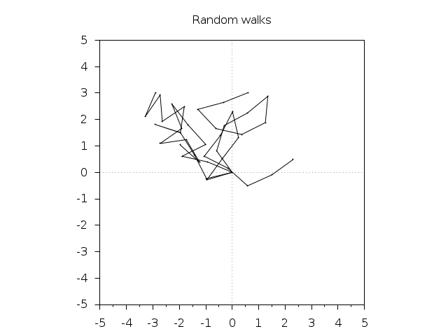
Fig. 5 Four 10-step random walks from the origin.
The following program computes the upper and lower cumulative
distribution functions for the standard normal distribution at
 .
.
#include <stdio.h>
#include <gsl/gsl_cdf.h>

int
main (void)
{
  double P, Q;
  double x = 2.0;

  P = gsl_cdf_ugaussian_P (x);
  printf ("prob(x < %f) = %f\n", x, P);

  Q = gsl_cdf_ugaussian_Q (x);
  printf ("prob(x > %f) = %f\n", x, Q);

  x = gsl_cdf_ugaussian_Pinv (P);
  printf ("Pinv(%f) = %f\n", P, x);

  x = gsl_cdf_ugaussian_Qinv (Q);
  printf ("Qinv(%f) = %f\n", Q, x);

  return 0;
}
Here is the output of the program,
prob(x < 2.000000) = 0.977250
prob(x > 2.000000) = 0.022750
Pinv(0.977250) = 2.000000
Qinv(0.022750) = 2.000000
References and Further Reading
For an encyclopaedic coverage of the subject readers are advised to consult the book “Non-Uniform Random Variate Generation” by Luc Devroye. It covers every imaginable distribution and provides hundreds of algorithms.
Luc Devroye, “Non-Uniform Random Variate Generation”, Springer-Verlag, ISBN 0-387-96305-7. Available online at http://cg.scs.carleton.ca/~luc/rnbookindex.html.
The subject of random variate generation is also reviewed by Knuth, who describes algorithms for all the major distributions.
Donald E. Knuth, “The Art of Computer Programming: Seminumerical Algorithms” (Vol 2, 3rd Ed, 1997), Addison-Wesley, ISBN 0201896842.
The Particle Data Group provides a short review of techniques for generating distributions of random numbers in the “Monte Carlo” section of its Annual Review of Particle Physics.
Review of Particle Properties, R.M. Barnett et al., Physical Review D54, 1 (1996) http://pdg.lbl.gov/.
The Review of Particle Physics is available online in postscript and pdf format.
An overview of methods used to compute cumulative distribution functions can be found in Statistical Computing by W.J. Kennedy and J.E. Gentle. Another general reference is Elements of Statistical Computing by R.A. Thisted.
William E. Kennedy and James E. Gentle, Statistical Computing (1980), Marcel Dekker, ISBN 0-8247-6898-1.
Ronald A. Thisted, Elements of Statistical Computing (1988), Chapman & Hall, ISBN 0-412-01371-1.
The cumulative distribution functions for the Gaussian distribution are based on the following papers,
Rational Chebyshev Approximations Using Linear Equations, W.J. Cody, W. Fraser, J.F. Hart. Numerische Mathematik 12, 242–251 (1968).
Rational Chebyshev Approximations for the Error Function, W.J. Cody. Mathematics of Computation 23, n107, 631–637 (July 1969).